---
title: "Lecture 9: Joining multiple datasets"
subtitle: "Managing and Manipulating Data Using R"
author:
date:
urlcolor: blue
output:
html_document:
toc: true
toc_depth: 2
#toc_float: # toc_float option to float the table of contents to the left of the main document content. floating table of contents will always be visible even when the document is scrolled
#collapsed: false # collapsed (defaults to TRUE) controls whether the TOC appears with only the top-level (e.g., H2) headers. If collapsed initially, the TOC is automatically expanded inline when necessary
#smooth_scroll: true # smooth_scroll (defaults to TRUE) controls whether page scrolls are animated when TOC items are navigated to via mouse clicks
number_sections: true
fig_caption: true # ? this option doesn't seem to be working for figure inserted below outside of r code chunk
highlight: tango # Supported styles include "default", "tango", "pygments", "kate", "monochrome", "espresso", "zenburn", and "haddock" (specify null to prevent syntax
theme: default # theme specifies the Bootstrap theme to use for the page. Valid themes include default, cerulean, journal, flatly, readable, spacelab, united, cosmo, lumen, paper, sandstone, simplex, and yeti.
df_print: tibble #options: default, tibble, paged
keep_md: true # may be helpful for storing on github
---
```{r, echo=FALSE}
#DON'T WORRY ABOUT THIS CODE
knitr::opts_chunk$set(collapse = TRUE, comment = "#>", highlight = TRUE)
```
```{r, echo=FALSE, include=FALSE}
#DO NOT WORRY ABOUT THIS
if(!file.exists('join-setup.png')){
download.file(url = 'https://github.com/ozanj/rclass/raw/master/lectures/lecture7/join-setup.png',
destfile = 'join-setup.png',
mode = 'wb')
}
```
```{r echo=FALSE, include=FALSE}
if(!file.exists('join-inner.png')){
download.file(url = 'https://github.com/ozanj/rclass/raw/master/lectures/lecture7/join-inner.png',
destfile = 'join-inner.png',
mode = 'wb')
}
```
```{r echo=FALSE, include=FALSE}
if(!file.exists('join-many-to-one.png')){
download.file(url = 'https://github.com/ozanj/rclass/raw/master/lectures/lecture7/join-many-to-one.png',
destfile = 'join-many-to-one.png',
mode = 'wb')
}
```
```{r echo=FALSE, include=FALSE}
if(!file.exists('join-outer.png')){
download.file(url = 'https://github.com/ozanj/rclass/raw/master/lectures/lecture7/join-outer.png',
destfile = 'join-outer.png',
mode = 'wb')
}
```
```{r echo=FALSE, include=FALSE}
if(!file.exists('lecture1.2.R')){
download.file(url = 'https://github.com/ozanj/rclass/raw/master/lectures/lecture1/lecture1.2.R',
destfile = 'lecture1.2.R',
mode = 'wb')
}
```
# Introduction
## Logistics
### Reading
- Work through slides we from lecture 9 that we don't get to in class
- [REQUIRED] slides through the section on "Join problems"
- [OPTIONAL] section on "Appending/stacking data"
- [RECOMMENDED] GW chapter 13 (Relational data)
- Lecture 9 covers this material pretty closely. Please read chapter if you can, but I get it if you don't have time
### Problem set
For problem set due next week, you will submit an R "script" (has extension ".R") rather than an RMarkdown file (has extension ".Rmd")
- For most research projects, people write scripts rather than .Rmd files, so we want to practice doing this.
- We will give you an R script that have code created by us that you can run. And then you will write code answering questions posed in the problem set.
An R script is just a text file full of R commands
- Can create "comments" by using "#"
- Shortcuts for executing commands
- __Cmd/Ctrl + Enter__: execute highlighted line(s)
- __Cmd/Ctrl + Shift + Enter__ (without highlighting any lines): run entire script
- Output from commands executed from R script
- Output will appear in the "console"
- Link to a very simple R script
- [HERE](Lecture1.2.R)
### Mid-quarter evaluation
Some of the constructive criticism
- Time on in-class practice problems
- 50% indicated time is about right, 37.5% not enough time, 12.5% too much time
- More real-world problem sets like GPA assignment or bonus questions that incorporate skills across different weeks
- Lecture is too long, possibly reviewing lectures as reading assignments, spend class time on key points/questions
- Future format will be online/in-person hybrid-- lectures will be recorded, students view on their own, 1 hr per week lab sessions
## Lecture overview
It is rare for an analysis dataset to consist of data from only one input dataset. For most projects, each analysis dataset contains data from multiple data sources. Therefore, you must become proficient in combining data from multiple data sources.
Two broad topics today:
1. __Joining__ datasets [big topic]
- Combine two datasets so that the resulting dataset has additional variables
- The term "join" comes from the relational databases world; Social science research often uses the term "merge" rather than "join"
2. __Appending__ datasets [small topic]
- Stack datasets on top of one another so that resulting dataset has more observations, but (typically) the same number of variables
- Often, longitudinal datasets are created by appending datasets
Wickham differentiates __mutating joins__ from __filtering joins__
- Mutating joins "add new variables to one data frame from matching observations in another"
- Filtering joins "filter observations from one data frame based on whether or not they match an observation in the other table"
- doesn't add new variables
Our main focus today is on _mutating joins_. But _Filtering joins_ are useful for data quality checks of _mutating joins_.
Libraries we will use
```{r}
library(tidyverse)
library(haven)
library(labelled)
```
## NLS72 data
Today's lecture will utilize several datasets from the National Longitudinal Survey of 1972 (NLS72):
- Student level dataset
- Student-transcript level dataset
- Student-transcript-term level dataset
- Student-transcript-term-course level dataset
These datasets are good for teaching "joining" because you get practice joining data sources with different "observational levels" (e.g., join student level and student-transcript level data)
### Read in NLS72 data frames
Below, we'll read-in Stata data files and keep a small number of variables from each. Don't worry about investigating individual variables, just get an overall sense of each data frame.
- __Student level data__
```{r}
rm(list = ls()) # remove all objects
#getwd()
nls_stu <- read_dta(file="https://github.com/ozanj/rclass/raw/master/data/nls72/nls72stu_percontor_vars.dta") %>%
select(id,schcode,bysex,csex,crace,cbirthm,cbirthd,cbirthyr)
#get a feel for the data
names(nls_stu)
glimpse(nls_stu)
nls_stu %>% var_label()
#we can investigate individual variables (e.g., bysex variable)
class(nls_stu$bysex)
str(nls_stu$bysex)
nls_stu %>% select(bysex) %>% var_label()
nls_stu %>% select(bysex) %>% val_labels()
nls_stu %>% count(bysex)
nls_stu %>% count(bysex) %>% as_factor()
```
- __Student level data, containing variables about completeness of postsecondary education transcripts (PETS)__
```{r}
nls_stu_pets <- read_dta(file="https://github.com/ozanj/rclass/raw/master/data/nls72/nls72petsstu_v2.dta") %>%
select(id,reqtrans,numtrans)
names(nls_stu_pets)
glimpse(nls_stu_pets)
nls_stu_pets %>% var_label()
```
- __Student-transcript level data__
```{r}
nls_tran <- read_dta(file="https://github.com/ozanj/rclass/raw/master/data/nls72/nls72petstrn_v2.dta") %>%
select(id,transnum,findisp,trnsflag,terms,fice,state,cofcon,instype,itype)
names(nls_tran)
glimpse(nls_tran)
nls_tran %>% var_label()
nls_tran %>% val_labels()
```
- __Student-transcript-term level data__
```{r}
nls_term <- read_dta(file="https://github.com/ozanj/rclass/raw/master/data/nls72/nls72petstrm_v2.dta") %>%
select(id,transnum,termnum,courses,termtype,season,sortdate,gradcode,transfer)
names(nls_term)
glimpse(nls_term)
nls_term %>% var_label()
nls_term %>% val_labels()
```
- __Student-transcript-term-course level data__
- This is the file we worked with for the "create GPA" problem set
```{r}
nls_course <- read_dta(file="https://github.com/ozanj/rclass/raw/master/data/nls72/nls72petscrs_v2.dta") %>%
select(id,transnum,termnum,crsecip,crsecred,gradtype,crsgrada,crsgradb)
names(nls_course)
glimpse(nls_course)
nls_course %>% var_label()
#nls_course %>% val_labels() # output too long!
```
## Relational databases and tables
__Traditionally, social scientists store data in "flat files"__
- flat files are "rectangular" datasets consisting of columns (usually called variables) and rows (usually called observations)
- When we want to incorporate variables from two flat files, we "merge" them together.
__The rest of the world stores data in "relational databases"__
- A relational database consists of multiple __tables__
- Each table is a flat file
- A goal of relational databases is to store data using the minimum possible space; therefore, a rule is to never duplicate information across tables
- When you need information from multiple tables, you "join"(the database term for "merge") tables "on the fly" rather than creating some permanent flat file that contains data from multiple tables
- Each table in a relational database has a different "observational level"
- For example, NLS72 has a student level table, a student-transcript level table, etc.
- From the perspective of a database person, it wouldn't make sense to store student level variables (e.g., birth-date) on the student-transcript level table because student birth-date does not vary by transcript, so this would result in needless duplication of data
- Structured Query Language (SQL) is the universally-used programming language for relational databases
__Real-world examples of relational databases__
- iTunes
- Behind the scenes, there are separate tables for artist, album, song, genre, etc.
- The "library" you see as a user is the result of "on the fly" joins of these tables
- Every social media app (e.g., twitter, fb, gram) you use is a relational database;
- What you see as a user is the result of "on the fly" joins of individual tables running in the background
- Interactive maps typically have relational databases running in the background
- Clicking on some part of the map triggers a join of tables and you see the result of some analysis based on that join
- e.g., our [off-campus recruiting map](https://map.emraresearch.org/)
- [show SQL tables NaviCat/SequelPro]
Should you think of combining data-frames in R as "merging" flat-files or "joining" tables of a relational database?
- Can think of it either way; but I think better to think of it _both_ ways
- For example, you can think of the NLS72 datasets as:
- a bunch of flat-files that we merge
- OR a set of tables that comprise a relational database
- Although we are combining flat-files, tidyverse uses the terminology (e.g, "keys," "join") of relational databases for doing so
# Keys
__Keys__ are "the variables used to connect each pair of tables" in a relational database
__An important thing to keep in mind before we delve into an in-depth discussion of keys__
- Even though relational databases often consist of many tables, __relations__ are always defined between a __pair__ of tables
- When joining tables, focus on joining __one__ table to __another__; you make this "join" using the __key variable(s)__ that define the relationship between these two tables
- Even when your analysis requires variables from more than two tables, you proceed by joining one pair of tables at a time
__Definition of keys__
- Wickham: "A key is a variable (or set of variables) that uniquely identifies an observation"
- In other words, no two observations in the dataset have the same value of the key
In the simplest case, a single variable uniquely identifies observations and, thus, the key is simply that variable
- e.g., the variable `id` -- "unique student identification variable" -- uniquely identifies observations in the dataset `nls_stu`
- No two observations in `nls_stu` have the same value of `id`
Let's confirm that each value of `id` is associated with only one observation
```{r}
#approach A: create a variable that counts how many rows there are for each unique value of your candidate key
nls_stu %>% group_by(id) %>% # group by your candidate key
summarise(n_per_id=n()) %>% # create a measure of number of observations per group
ungroup %>% # ungroup, otherwise frequency table [next step] created separately for each group
count(n_per_id) # frequency of number of observations per group
#approach B: count how many values of id have more than one observation per id
nls_stu %>%
count(id) %>% # create object that counts the number of obs for each value of id
filter(n>1) # keep only rows where count of obs per id is greater than 1
```
- Approach B is simpler from a coding perspective, but I prefer Approach A
__Often, multiple variables are required to create the key for a table__
Ttask: confirm that the variables `id` and `transnum` form the key for the table `nls_tran`
```{r}
nls_tran %>% group_by(id,transnum) %>% summarise(n_per_key=n()) %>% ungroup %>% count(n_per_key)
nls_tran %>% count(id,transnum) %>% filter(n>1)
```
__The first step before merging a pair of tables is always to identify the key for each table__. We have already identified the key for `nls_stu` and `nls_tran`.
__Student Task__:
- try to identify the key for `nls_stu_pets`, `nls_term` and for `nls_course`
```{r}
#nls_stu_pets
nls_stu_pets %>% group_by(id) %>% summarise(n_per_key=n()) %>% ungroup %>% count(n_per_key)
#nls_term
nls_term %>% group_by(id,transnum,termnum) %>% summarise(n_per_key=n()) %>% ungroup %>% count(n_per_key)
#nls_course; key doesn't exist
nls_course %>% group_by(id,transnum,termnum,crsecip) %>% summarise(n_per_key=n()) %>% ungroup %>% count(n_per_key)
```
The dataset `nls_course` doesn't have a key! That is, there is no combination of variables that uniquely identifies each observation in `nls_course`.
When a table doesn't have a key, you can create one. This is called a __surrogate__ key
```{r}
nls_course_temp <- nls_course %>% group_by(id,transnum,termnum) %>%
mutate(coursenum=row_number()) %>% ungroup
nls_course_temp %>% group_by(id,transnum,termnum,coursenum) %>%
summarise(n_per_key=n()) %>% ungroup %>% count(n_per_key)
rm(nls_course_temp)
```
## Primary keys and foreign keys
So far, our discussion of keys has focused on a single table.
As we consider the relationship between tables, there are two types of keys, __primary key__ and __foreign key__:
### Primary key
__Definition of primary key__:
- a variable (or combination of variables) in a table that uniquely identifies observations in its own table
- this definition is the same as our previous definition for __key__
__Examples of primary keys:__
- e.g., `id` is the _primary key_ for the dataset `nls_stu`
```{r}
nls_stu %>% group_by(id) %>% summarise(n_per_key=n()) %>% ungroup %>% count(n_per_key)
```
- e.g., `id` and `transnum` form the _primary key_ for the dataset `nls_trans`
```{r}
nls_tran %>% group_by(id,transnum) %>% summarise(n_per_key=n()) %>% ungroup %>% count(n_per_key)
```
- But note that the dataset `nls_course` did not have a _primary key_
```{r}
nls_course %>% group_by(id,transnum,termnum,crsecip) %>% summarise(n_per_key=n()) %>% ungroup %>% count(n_per_key)
```
### Foreign key
__Definition of foreign key__:
- A variable (or combination of variables) in a table that uniquely identify observations in another table
- Said differently, a foreign key is a variable (or combination of variables) in a table that is the primary key in another table
Personally, I find the concept __foreign key__ a little bit slippery. Here is how I wrap my head around it:
- First, always remember that "joins" happen between two specific tables, so have two specific tables in mind
- Second, to understand _foreign key_ concept, I think of a "focal table" [my term] (e.g., `nls_tran`) and some "other table" (e.g., `nls_stu`).
- Third, then, the foreign key is a variable (or combination of variables) that satisfies two conditions (A) and (B):
- (A) exists in the "focal table" (but may or may not be the primary key for the focal table)
- (B) exists in the "other table" __AND__ is the primary key for that "other table"
__Example of foreign key__
- With respect to the "focal table" `nls_tran` and the "other table" `nls_stu`, the variable `id` is the _foreign key_ because:
- `id` exists in the "focal table" `nls_trans` (though it does not uniquely identifies observations in `nls_trans`)
- `id` exists in the "other table" `nls_stu` and `id` uniquely identifies observations in `nls_stu`
```{r}
nls_tran %>% group_by(id) %>% summarise(n_per_key=n()) %>% ungroup %>% count(n_per_key)
nls_stu %>% group_by(id) %>% summarise(n_per_key=n()) %>% ungroup %>% count(n_per_key)
```
__Example of foreign key__
- With respect to the "focal table" `nls_term` and the "other table" `nls_trans`, the variables `id` and `transnum` form the _foreign key_ because:
- These variables exists in the "focal table" `nls_term,` (though they do not uniquely identifies observations in `nls_term`)
- These variables exist in the "other table" `nls_tran` and they uniquely identifies observations in `nls_tran`
```{r}
nls_term %>% group_by(id,transnum) %>% summarise(n_per_key=n()) %>% ungroup %>% count(n_per_key)
nls_tran %>% group_by(id,transnum) %>% summarise(n_per_key=n()) %>% ungroup %>% count(n_per_key)
```
In practice, you join two tables without explicit thinking about "primary key" vs. "foreign key" and "focal table" vs. "other table"
- Doesn't matter wich data frame you "start with" (e.g., as the "focal table")
- The only requirements for joining are:
1. One of the two data frames have a __primary key__ (variable or combination of variables that uniquely identify observations) __AND__
1. That variable or combination of variables is available in the other of the two data frames
# Mutating joins
## Overview of mutating joins
Following Wickham, we'll explain joins by creating hypothetical tables `x` and `y`
```{r}
x <- tribble(
~key, ~val_x,
1, "x1",
2, "x2",
3, "x3"
)
y <- tribble(
~key, ~val_y,
1, "y1",
2, "y2",
4, "y3"
)
x
y
```
A __join__ "is a way of connecting each row in `x` to zero, one, or more rows in `y`"
Observations in table `x` matched to observations in table `y` using a "key" variable
- A key is a variable (or combination of variables) that exist in both tables and uniquely identifies observations in at least one of the two tables
Two tables `x` and `y` can be "joined" when the primary key for table `x` can be found in table `y`; in other words, when table `y` contains the _foreign key_, which uniquely identifies observations in table `x`
- e.g., use `id` to join `nls_stu` and `nls_tran` because `id` is the primary key for `nls_stu` (i.e., uniquely identifies obs in `nls_stu`) and `id` can be found in `nls_tran`
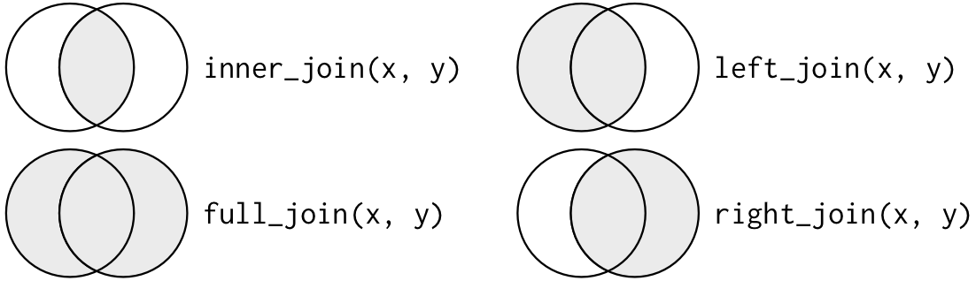
There are four types of joins between tables `x` and `y`:
- __inner join__: keep all observations that appear in both table `x` and table `y`
- __left join__: keep all observations in `x` (regardless of whether these obs appear in `y`)
- __right join__: keep all observations in `y` (regardless of whether these obs appear in `x`)
- __full join__: keep all observations that appear in `x` or in `y`
The last three joins -- left, right, full -- keep observations that appear in at least one table and are collectively referred to as __outer joins__
The following Venn diagram -- copied from Grolemund and Wickham Chapter 13 -- is useful for developing an initial understanding of the four join types
We will join tables `x` and `y` using the `join()` command from `dplyr` package. `join()` is a general command, which has more specific commands for each type of join:
- `inner_join()`
- `left_join()`
- `right_join()`
- `full_join()`
Note that all of these join commands result in an object that contains __all__ the variables from `x` and all the variables from `y`
- So if you want resulting object to contain a subset of variables from `x` and `y`, then prior to the join, you should eliminate unwanted variables from `x` and/or `y`
### How we'll teach joins
- I'll spend the most amount of time on __inner joins__, e.g., moving from simpler to more complicated joins.
- I'll spend less time on __outer joins__ because most of the stuff from inner joins will apply to outer joins too
- Note: all of the cool, multi-colored visual representations of joins are copied __directly__ from Grolemund and Wickham, Chapter 12)
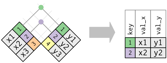
## Inner joins
__inner joins__ keep all observations that appear in both table `x` and table `y`
- More correctly, an inner join mathes observations from two tables "whenever their keys are equal"
- If there are multiple matches between `x` and `y`, all combination of the matches are returned.
- e.g., if object `x` has one row where the variable `key==1` and object `y` has two rows where the variable `key==1`, the resulting object will contain two rows where the variable `key==1`
Visual representation of `x` and `y`:
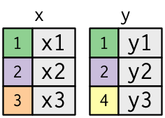
- the colored column in each dataset is the "key" variable. The key variable(s) match rows between the tables.
Below is a visual representation of an inner join.
- Matches in a join (rows common to both `x` and `y`) are indicated with dots. "The number of dots=the number of matches=the number of rows in the output"
The basic synatx in R: `inner_join(x, y, by ="keyvar")`
- where `x` and `y` are names of tables to join
- `by` specifies the name of the key variable or the combination of variables that form the key
```{r}
x
y
#inner_join (without pipes)
inner_join(x,y, by = "key")
#inner_join (with pipes)
x %>%
inner_join(y, by = "key")
```
__Practical example__:
- let's try an inner join of the two datasets `nls_stu` and `nls_stu_pets`
I recommend these general steps when merging two datasets
1. Identify `key` variable for `join()` command by investigating the data structure of each dataset. Do stuff like this:
- which variables uniquely identify obs (i.e., what is the "key" in each table)
- note: not all tables have keys
- Once you identify the primary key for one of the tables, make sure that variable (or combination of variables) exists in the other table
- Identify key variables you will use to join the two tables
2. Join datasets
3. Assess/investigate quality of join
- This is basically exploratory data analysis for the purpose of data quality
- e.g., for obs that don't "match", investigate why (what are the patterns)
- We talk about these investigations in more detail below in section on __filtering joins__ and section on __join problems__
__Task__: inner join of the two datasets `nls_stu` and `nls_stu_pets`
```{r}
#investigate data structure
nls_stu %>% group_by(id) %>% summarise(n_per_id=n()) %>% ungroup %>% count(n_per_id)
nls_stu_pets %>% group_by(id) %>% summarise(n_per_id=n()) %>% ungroup %>% count(n_per_id)
#id is primary key for both datasets, so use id as key variable
nls_stu_stu <- nls_stu %>%
inner_join(nls_stu_pets, by = "id")
names(nls_stu_stu)
nrow(nls_stu)
nrow(nls_stu_pets)
nrow(nls_stu_stu)
```
### one-to-one join vs. one-to-many join
Note: Wickham refers to the concepts in this section as "duplicate keys"
General rule rule of thumb for joining two tables
- __key variable must uniquely identify observations in at least one of the tables you are joining__
Depending on whether the key variable uniquely identifies observations in table `x` and/or table `y` you will have:
- __one-to-one__ join: key variable uniquely identifies observations in table `x` and uniquely identifies observations in table `y`
- The join between `nls_stu` and `nls_stu_pets` was a one-to-one join; the variable `id` uniquely identifies observations in both tables
- In the relational database world one-to-one joins are rare and are considered special cases of one-to-many or many-to-one joins
- Why? if tables can be joined via one-to-one join, then they should already be part of the same table.
- __one-to-many__ join: key variable uniquely identifies observatiosn in table `x` and does not uniquely identify observations in table `y`
- each observation from table `x` may match to multiple observations from table `y'
- e.g., `inner_join(nls_stu, nls_trans, by = "id")`
- e.g. _one_ observation (student) in `nls_stu` has _many_ observations in `nls_trans` (transcripts)
- __many-to-one__ join: key variable does not uniquely identify observations in table `x` and does uniquely identify observations in table `y`
- each observation from table `y` may match to multiple observations from table `x'
- e.g., `inner_join(nls_trans, nls_trans, by = "id")`
- e.g., _many_ observations (transcripts) in `nls_trans` have _one_ observation in `nls_stu` (student)
- __many-to-many__ join: key variable does not uniquely identify observations in table `x` and does not uniquely identify observations in table `y`
- This is usually an error
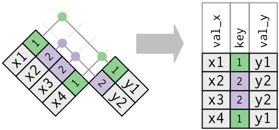
Many-to-one merge using fictitious tables `x` and `y`
```{r}
#create new versions of table x and table y
x <- tribble(
~key, ~val_x,
1, "x1",
2, "x2",
2, "x3",
1, "x4"
)
y <- tribble(
~key, ~val_y,
1, "y1",
2, "y2"
)
x
y
```
Step 1: Investigate the two tables
- Note that `key` does not uniquely identify observations in `x` but does uniquely identify observations in `y`
```{r}
x %>% group_by(key) %>% summarise(n_per_key=n()) %>% ungroup %>% count(n_per_key)
y %>% group_by(key) %>% summarise(n_per_key=n()) %>% ungroup %>% count(n_per_key)
```
Visual representation of merge
Step 2: "join" the two tables
```{r}
left_join(x, y, by = "key")
```
__Student-task__:
- conduct a one-to-many inner join of the two datasets `nls_stu` and `nls_trans`
Fine to try doing it without looking at solutions, or just work through solutions below
__Solution to student task__: steps
1. Invesigate data structure
2. Join variables
3. Assess/investigate quality of join
```{r}
#Investigate data
#we know id is primary key for nls_stu, investigate primary key for nls_tran
#id does not uniquely identify obs in nls_tran
nls_tran %>% group_by(id) %>% summarise(n_per_key=n()) %>% ungroup %>%
filter(n_per_key>1) %>% count(n_per_key)
#id and transnum uniquely identify obs
nls_tran %>% group_by(id,transnum) %>% summarise(n_per_key=n()) %>% ungroup %>%
filter(n_per_key>1) %>% count(n_per_key)
#id uniquely identifies obs in nls_stu and id is available in nls_tran, so use id as key
#merge
nls_stu_tran <- nls_stu %>% inner_join(nls_tran, by = "id") #error warning on var labels will populate
#investigate results of merge
names(nls_stu_tran)
nrow(nls_stu)
nrow(nls_tran)
nrow(nls_stu_tran)
#Below sections show how to investigate quality of merge in more detail
```
### Defining the key columns
Thus far, tables have been joined by a single "key" variable using this syntax:
- `inner_join(x,y, by = "keyvar")`
Often, multiple variables form the "key". Specify this using this syntax:
- `inner_join(x,y, by = c("keyvar1","keyvar2","..."))`
__Practical example__:
- perform an inner join of `nls_tran` and `nls_term`
```{r}
#Investigate
nls_tran %>% group_by(id,transnum) %>% summarise(n_per_key=n()) %>% ungroup %>%
filter(n_per_key>1) %>% count(n_per_key)
nls_term %>% group_by(id,transnum,termnum) %>% summarise(n_per_key=n()) %>% ungroup %>%
filter(n_per_key>1) %>% count(n_per_key)
#merge
nls_tran_term <- nls_tran %>% inner_join(nls_term, by = c("id","transnum"))
#investigate
nrow(nls_tran)
nrow(nls_term)
nrow(nls_tran_term)
#appears that some observations from nls_term did not merge with nls_trans
#we should investigate this further [below]
```
Sometimes a key variable in one table has a different variable name in the other table. You can specify that the variables to be matched from one table to another as follows:
- `inner_join(x,y, by = c("keyvarx" = "keyvary"))`
__Practical example__:
- perform inner join between `nls_stu` and `nls_tran`:
```{r}
#we've seen this code before
nls_stu_tran <- nls_stu %>% inner_join(nls_tran, by = "id")
#but this code works too
nls_stu_tran <- nls_stu %>% inner_join(nls_tran, by = c("id" = "id"))
#and this code would work too
nls_stu_tran <- nls_stu %>% rename(idv2=id) %>% # rename id var in nls_stu
inner_join(nls_tran, by = c("idv2" = "id"))
```
Same syntax can be used when key is formed from multiple variables
- show using merge of `nls_tran` and `nls_term`
```{r}
#we've seen this code before
nls_tran_term <- nls_tran %>% inner_join(nls_term, by = c("id","transnum"))
#this code works too
nls_tran_term <- nls_tran %>% inner_join(nls_term, by = c("id" = "id","transnum" = "transnum"))
#and so does this
nls_tran_term <- nls_tran %>% rename(transnumv2=transnum) %>%
inner_join(nls_term, by = c("id" = "id","transnumv2" = "transnum"))
```
## Outer joins
Thus far we have focused on "inner joins"
- keep all observations that appear in both table `x` and table `y`
"outer joins" keep observations that appear in at least one table. There are three types of outer joins:
- __left join__: keep all observations in `x` (regardless of whether these obs appear in `y`)
- __right join__: keep all observations in `y` (regardless of whether these obs appear in `x`)
- __full join__: keep all observations that appear in `x` or in `y`
### Description of the four join types from R help file
The syntax for the outer join commands is identical to inner joins, so once you understand inner joins, outer joins are not difficult.
- `inner_join()`
- return all rows from x where there are matching values in y, and all columns from x and y. If there are multiple matches between x and y, all combination of the matches are returned.
- `left_join()`
- return all rows from x, and all columns from x and y. Rows in x with no match in y will have NA values in the new columns. If there are multiple matches between x and y, all combinations of the matches are returned.
- `right_join()`
- return all rows from y, and all columns from x and y. Rows in y with no match in x will have NA values in the new columns. If there are multiple matches between x and y, all combinations of the matches are returned.
- `full_join()`
- return all rows and all columns from both x and y. Where there are not matching values, returns NA for the one missing.
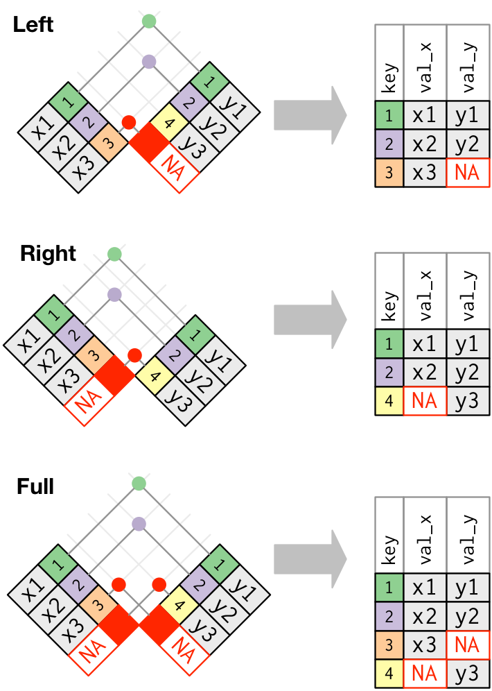
### Visual representation of outer joins
This figures are copied straight from Wickham chapter 12
__Venn diagram of joins__

__We want to perform outer joins on these two tables__

__Visual representation of outer joins__
"These joins work by adding an additional “virtual” observation to each table. This observation has a key that always matches (if no other key matches), and a value filled with NA."
### Practicing outer joins
The left-join is the most commonly used outer join in social science research (more common than inner join too).
Why is this? Often, we start with some dataset `x` (e.g., `nls_stu`) and we want to add variables from dataset `y`
- Usually, we want to keep observations from `x` regardless of whether they match with `y`
- Usually uninterested in observations from `y` that did not match with `x`
__Student task__ (try doing yourself or just follow along):
- start with `nls_stu_pets`
- perform a left join with `nls_stu` and save the object
- Then perform a left join with `nls_tran`
```{r}
#investigate data structure of nls_stu_pets and nls_tran
nls_stu_pets %>% group_by(id) %>% summarise(n_per_key=n()) %>% ungroup %>% count(n_per_key)
nls_stu %>% group_by(id) %>% summarise(n_per_key=n()) %>% ungroup %>% count(n_per_key)
#left merge w/ nls_stu_pets as x table and nls_tran as y table
nls_stu_pets_stu <- nls_stu_pets %>%
left_join(nls_stu, by = "id")
#investigate data structure of merged object
nrow(nls_stu_pets)
nrow(nls_stu)
nrow(nls_stu_pets_stu)
#investigate data structure of nls_stu_pets and nls_tran
nls_tran %>% group_by(id,transnum) %>% summarise(n_per_key=n()) %>% ungroup %>% count(n_per_key)
#merge nls_stu_pets_stu with nls_tran
nls_stu_pets_stu_tran <- nls_stu_pets_stu %>%
left_join(nls_tran, by = "id")
#investigate data structure of merged object
nrow(nls_stu_pets_stu)
nrow(nls_tran)
nrow(nls_stu_pets_stu_tran) # 3 more obs in resulting dataset than in nls_tran
```
# Filtering joins
__Filtering joins__ are very similar to _mutating joins_.
Filtering joins affect which observations are retained in the resulting object, but not which variables are retained
There are two types of filtering joins, `semi_join()` and `anti_join()`. Here are their descriptions from `?join`:
- `anti_join(x, y)`
- return all rows from x where there are not matching values in y, keeping just columns from x
- `semi_join(x, y)`
- return all rows from x where there are matching values in y, keeping just columns from x.
Difference between a `semi_join()` and an `inner_join()` in terms of which observations are present in the resulting object:
- Imagine that if object `x` has one row with `key==4` and object `y` has two rows with `key==4`'
- __inner_join__: resulting object will have two rows with `key==4`
- __semi_join__: resulting object will have one row with `key==4`
- Why? __because the rule for `semi_join` is to never duplicate rows of x__
Note: syntax for `semi_join()` and `anti_join()` follows the exact same patterns as syntax for mutating joins (e.g., `inner_join()` `left_join`)
## Using `anti_join()` to diagnose mismatches in mutating joins
A primary use of filtering joins is as an investigative tool to diagnose problems with mutating joins
__Practical example__: Investigate observations that don't match from `inner_join()` of `nls_tran` and `nls_course`
- transcript data has info on postsecondary transcripts; course data has info on each course in postsecondary transcript
```{r}
#assert that id and transnum uniquely identify obs in nls_trans
nls_tran %>% group_by(id,transnum) %>% summarise(n_per_key=n()) %>% ungroup %>% count(n_per_key)
#join data frames
nls_tran %>% inner_join(nls_course, by = c("id","transnum")) %>% count()
#compare to count of number of obs in nls_course
nls_course %>% count()
#difficult to tell which obs from nls_tran didn't merge
#use ant_join to isolate obs from nls_tran that didn't have match in nls_course
nls_tran %>% anti_join(nls_course, by = c("id","transnum")) %>% count()
#create object of obs that didn't merge
tran_course_anti <- nls_tran %>% anti_join(nls_course, by = c("id","transnum"))
names(tran_course_anti)
tran_course_anti %>% select(findisp) %>% var_label()
tran_course_anti %>% select(findisp) %>% count(findisp)
tran_course_anti %>% select(findisp) %>% val_labels()
tran_course_anti %>% select(findisp) %>% count(findisp) %>% as_factor()
```
__Practical example__: perform an inner-join of `nls_tran` and `nls_course` and a semi-join of `nls_tran` and `nls_course`.
- How do the results of these two joins differ?
- How can this semi-join be practically useful?
```{r}
#inner join
inner_tran_course <- nls_tran %>% inner_join(nls_course, by = c("id","transnum"))
#semi-join
semi_tran_course <- nls_tran %>% semi_join(nls_course, by = c("id","transnum"))
#anti-join
anti_tran_course <- nls_tran %>% anti_join(nls_course, by = c("id","transnum"))
inner_tran_course %>%
group_by(id, transnum) %>%
count()
semi_tran_course %>%
group_by(id, transnum) %>%
count()
anti_tran_course %>%
group_by(id, transnum) %>%
count()
```
- How do the results of these two joins differ?
- semi-join contains obs from `x` that matched with `y` [nls_course] but does not repeat rows of x
- semi-join only retains columns from `x`
- How can this semi-join be practically useful?
- semi-join could be useful when used in conjunction with anti-join to check observations that matched and did not match for `x`
__Let's see how this works with a smaller dataframe:__
```{r}
x <- tribble(
~key, ~val_x,
1, "x1",
2, "x2",
2, "x3",
1, "x4",
3, "x5",
4, "x6",
5, "x7",
6, "x8"
)
y <- tribble(
~key, ~val_y,
1, "y1",
2, "y2",
3, "y3",
4, "y4",
9, "y5"
)
x
y
```
What are the differences between different joins?
```{r}
inner_join(x,y, by = "key") #Return all rows from x where there are matching values in y
left_join(x, y, by = "key") #Return all rows from x, and all columns from x and y
semi_join(x,y, by = "key") #Return all rows from x where there are matching values in y, keeping just columns from x
anti_join(x,y, by = "key") #Return all rows from x where there are not matching values in y, keeping just columns from x
```
- semi-join and anti-join could be particularly useful for inner and left joins.
# Join problems
- How to avoid join problems before they arise.
- How to overcome join problems when they do arise
## Overcoming join problems before they arise
1. Start by investigating the data structure of tables you are going to merge
- identify the primary key in each table.
- This investigation should be based on your understanding of the data and reading data documentation rather than checking if each combination of variables is a primary key
- does either table have missing or strange values (e.g., `-8`) for the primary key; if so, these observations won't match
1. Before joining, make sure that key you will use for joining uniquely identifies observations in at least one of the datasets and that the key variable(s) is present in both datasets
- investigate whether key variables have different names across the two tables. If different, then you will have to adjust syntax of your join statement accordingly
1. Before joining, you also want to make sure the key variable in one table and key variable in another table are the same type (both numeric, or both string, etc.)
- You could use the `typeof` function or the `str` function
- Change type with this command `x$key <- as.double(x$key)` or `x$key <- as.character(x$key)`
- If you try to join with key variables of different type, you will get this error message: Can't join on 'key' x 'key' because of incompatible types (character / numeric)
1. Think about which observations you want retained after joining
- think about which dataset should be the `x` table and which should be the `y` table
- think about whether you want an inner, left, right, or full join
1. Since mutating joins keep all variables in `x` and `y`, you may want to keep only specific variables in `x` and/or `y` as a prior step to joining
- Make sure that non-key variables from tables have different names; if duplicate names exist, the default is to add `.x and .y` to the end of the variable name. For example, if you have two tables with non-key variables with the name `type` and you join them, you will end up with variables(columns) `type.x` and `type.y`.
## Overcoming join problems when they do arise
- Identify which observations don't match
- `anti_join()` is your friend here
- Investigate the reasons that observations don't match
- Investigating joins is a craft that takes some practice getting good at; this is essentially an exercise in exploratory data analysis for the purpose of data quality
- First, you have to _care_ about data quality
- Identifying causes for non-matches usually involves consulting data documentation for both tables and performing basic descriptive statistics (e.g., frequency tables) on specific variables that documentation suggests may be relevant for whether obs match or not
# Appending/stacking data
Often we want to "stack" multiple datasets on top of one another
- typically datasets have the same variables, so stacking means that number of variables remains the same but number of observations increases
We append data using the `bind_rows()` function, which is from the _dplyr_ package
```{r}
#?bind_rows
time1 <- tribble(
~id, ~year, ~income,
1, 2017, 50,
2, 2017, 100,
3, 2017, 200
)
time2 <- tribble(
~id, ~year, ~income,
1, 2018, 70,
2, 2018, 120,
3, 2018, 220
)
time1
time2
append_time <- bind_rows(time1,time2)
append_time
append_time %>% arrange(id,year)
```
Most common practical use of stacking is creating "longitudinal dataset" when input data are released separately for each time period
- longitudinal data has one row per time period for a person/place/observation
__Practical Example__:
- IPEDS collects annual survey data from colleges/universities
- Create longitudinal data about university characteristics by appending/staking annual data
Load annual IPEDS data on admissions characteristics
```{r}
admit16_17 <- read_dta(file="https://github.com/ozanj/rclass/raw/master/data/ipeds/ic/ic16_17_admit.dta") %>%
select(unitid,endyear,sector,contains("admcon"),contains("numapply"),contains("numadmit"))
glimpse(admit16_17)
admit16_17 %>% var_label()
#admit16_17 %>% val_labels()
#read in previous two years of data
admit15_16 <- read_dta(file="https://github.com/ozanj/rclass/raw/master/data/ipeds/ic/ic15_16_admit.dta") %>%
select(unitid,endyear,sector,contains("admcon"),contains("numapply"),contains("numadmit"))
admit14_15 <- read_dta(file="https://github.com/ozanj/rclass/raw/master/data/ipeds/ic/ic14_15_admit.dta") %>%
select(unitid,endyear,sector,contains("admcon"),contains("numapply"),contains("numadmit"))
```
Appending/Stack IPEDS datasets
```{r, warning=FALSE}
admit_append <- bind_rows(admit16_17,admit15_16,admit14_15)
#note that R complains about preserving "labelled" data; does not retain labels
str(admit_append)
```
Investigate structure
```{r}
admit_append %>% select(unitid,endyear,admcon1,admcon2,numapplytot,numadmittot) %>%
arrange(unitid,endyear) %>% head(n=10)
#investigate data structure: one obs per unitid-endyear
admit_append %>% group_by(unitid,endyear) %>% summarise(n_per_key=n()) %>% ungroup %>% count(n_per_key)
```
__Appending when not all columns match__ results in NA for observations where columns do not match
```{r, warning=FALSE}
#read 15-16 data without numapply vars
admit15_16 <- read_dta(file="https://github.com/ozanj/rclass/raw/master/data/ipeds/ic/ic15_16_admit.dta") %>%
select(unitid,endyear,sector,contains("admcon"))
#read 14-15 data with numapply vars
admit14_15 <- read_dta(file="https://github.com/ozanj/rclass/raw/master/data/ipeds/ic/ic14_15_admit.dta") %>%
select(unitid,endyear,sector,contains("admcon"),contains("numapply"))
admit_append <- bind_rows(admit15_16,admit14_15)
admit_append %>% filter(endyear==2016) %>%
count(is.na(numapplytot))
admit_append %>% filter(endyear==2015) %>%
count(is.na(numapplytot))
```