# geos
[](https://cran.r-project.org/package=geos)
[](https://app.codecov.io/gh/paleolimbot/geos?branch=master)
[](https://github.com/paleolimbot/geos/actions)
The goal of geos is to provide access to the GEOS C API by vectorizing
the C functions for use in R. See the [package function
reference](https://paleolimbot.github.io/geos/reference/index.html) for
which functions are implemented in the R API.
## Installation
You can install the released version of geos from
[CRAN](https://CRAN.R-project.org) with:
``` r
install.packages("geos")
```
And the development version from [GitHub](https://github.com/) with:
``` r
# install.packages("remotes")
remotes::install_github("paleolimbot/geos")
```
If you can load the package, you’re good to go!
``` r
library(geos)
```
## Example
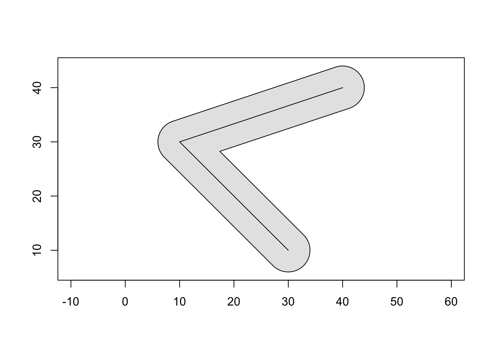
Buffer a line and plot it!
``` r
line <- as_geos_geometry("LINESTRING (30 10, 10 30, 40 40)")
plot(geos_buffer(line, distance = 4), col = "grey90")
plot(line, add = T)
```
 The geos package is designed to work with
[dplyr](https://dplyr.tidyverse.org/) package, so you can work with
geometry vectors as a data frame column:
``` r
library(dplyr)
#>
#> Attaching package: 'dplyr'
#> The following objects are masked from 'package:stats':
#>
#> filter, lag
#> The following objects are masked from 'package:base':
#>
#> intersect, setdiff, setequal, union
# map data from the maps package via ggplot2
states_df <- as_tibble(ggplot2::map_data("state"))
states_df
#> # A tibble: 15,537 × 6
#> long lat group order region subregion
#>
#> 1 -87.5 30.4 1 1 alabama
#> 2 -87.5 30.4 1 2 alabama
#> 3 -87.5 30.4 1 3 alabama
#> 4 -87.5 30.3 1 4 alabama
#> 5 -87.6 30.3 1 5 alabama
#> 6 -87.6 30.3 1 6 alabama
#> 7 -87.6 30.3 1 7 alabama
#> 8 -87.6 30.3 1 8 alabama
#> 9 -87.7 30.3 1 9 alabama
#> 10 -87.8 30.3 1 10 alabama
#> # … with 15,527 more rows
states_df %>%
group_by(region, group) %>%
summarise(geometry = geos_make_polygon(long, lat)) %>%
summarise(geometry = geos_make_collection(geometry, "multipolygon"))
#> `summarise()` has grouped output by 'region'. You can override using the
#> `.groups` argument.
#> # A tibble: 49 × 2
#> region geometry
#>
#> 1 alabama
#> 2 arizona
#> 3 arkansas
#> 4 california
#> 5 colorado
#> 6 connecticut
#> 7 delaware
#> 8 district of columbia
#> 9 florida
#> 10 georgia
#> # … with 39 more rows
```
The easiest way to get data into and out of the package is using the [sf
package](https://r-spatial.github.io/sf/).
``` r
library(sf)
#> Linking to GEOS 3.11.0, GDAL 3.5.1, PROJ 9.0.1; sf_use_s2() is TRUE
nc <- read_sf(system.file("shape/nc.shp", package = "sf")) %>%
st_transform(32119) # North Carolina state plane, m.
nc_geos <- as_geos_geometry(nc)
nc_geos %>%
geos_make_collection() %>%
geos_unary_union() %>%
st_as_sfc(nc_state)
#> Geometry set for 1 feature
#> Geometry type: MULTIPOLYGON
#> Dimension: XY
#> Bounding box: xmin: 123829 ymin: 14744.69 xmax: 930521.8 ymax: 318259.9
#> Projected CRS: NAD83 / North Carolina
#> MULTIPOLYGON (((138426 177699.3, 145548.6 17783...
```
The geos package is designed to work with
[dplyr](https://dplyr.tidyverse.org/) package, so you can work with
geometry vectors as a data frame column:
``` r
library(dplyr)
#>
#> Attaching package: 'dplyr'
#> The following objects are masked from 'package:stats':
#>
#> filter, lag
#> The following objects are masked from 'package:base':
#>
#> intersect, setdiff, setequal, union
# map data from the maps package via ggplot2
states_df <- as_tibble(ggplot2::map_data("state"))
states_df
#> # A tibble: 15,537 × 6
#> long lat group order region subregion
#>
#> 1 -87.5 30.4 1 1 alabama
#> 2 -87.5 30.4 1 2 alabama
#> 3 -87.5 30.4 1 3 alabama
#> 4 -87.5 30.3 1 4 alabama
#> 5 -87.6 30.3 1 5 alabama
#> 6 -87.6 30.3 1 6 alabama
#> 7 -87.6 30.3 1 7 alabama
#> 8 -87.6 30.3 1 8 alabama
#> 9 -87.7 30.3 1 9 alabama
#> 10 -87.8 30.3 1 10 alabama
#> # … with 15,527 more rows
states_df %>%
group_by(region, group) %>%
summarise(geometry = geos_make_polygon(long, lat)) %>%
summarise(geometry = geos_make_collection(geometry, "multipolygon"))
#> `summarise()` has grouped output by 'region'. You can override using the
#> `.groups` argument.
#> # A tibble: 49 × 2
#> region geometry
#>
#> 1 alabama
#> 2 arizona
#> 3 arkansas
#> 4 california
#> 5 colorado
#> 6 connecticut
#> 7 delaware
#> 8 district of columbia
#> 9 florida
#> 10 georgia
#> # … with 39 more rows
```
The easiest way to get data into and out of the package is using the [sf
package](https://r-spatial.github.io/sf/).
``` r
library(sf)
#> Linking to GEOS 3.11.0, GDAL 3.5.1, PROJ 9.0.1; sf_use_s2() is TRUE
nc <- read_sf(system.file("shape/nc.shp", package = "sf")) %>%
st_transform(32119) # North Carolina state plane, m.
nc_geos <- as_geos_geometry(nc)
nc_geos %>%
geos_make_collection() %>%
geos_unary_union() %>%
st_as_sfc(nc_state)
#> Geometry set for 1 feature
#> Geometry type: MULTIPOLYGON
#> Dimension: XY
#> Bounding box: xmin: 123829 ymin: 14744.69 xmax: 930521.8 ymax: 318259.9
#> Projected CRS: NAD83 / North Carolina
#> MULTIPOLYGON (((138426 177699.3, 145548.6 17783...
```