{
"cells": [
{
"cell_type": "markdown",
"metadata": {},
"source": [
"# DSI Summer Workshops Series\n",
"\n",
"## June 14, 2018\n",
"\n",
"Peggy Lindner
\n",
"Center for Advanced Computing & Data Science (CACDS)
\n",
"Data Science Institute (DSI)
\n",
"University of Houston \n",
"plindner@uh.edu \n",
"\n",
"\n",
"Please make sure you have Jupyterhub running with support for R and all the required packages installed.\n",
"Data for this and other tutorials can be found in the github repsoitory for the Summer 2018 DSI Workshops\n",
"https://github.com/peggylind/Materials_Summer2018\n"
]
},
{
"cell_type": "markdown",
"metadata": {},
"source": [
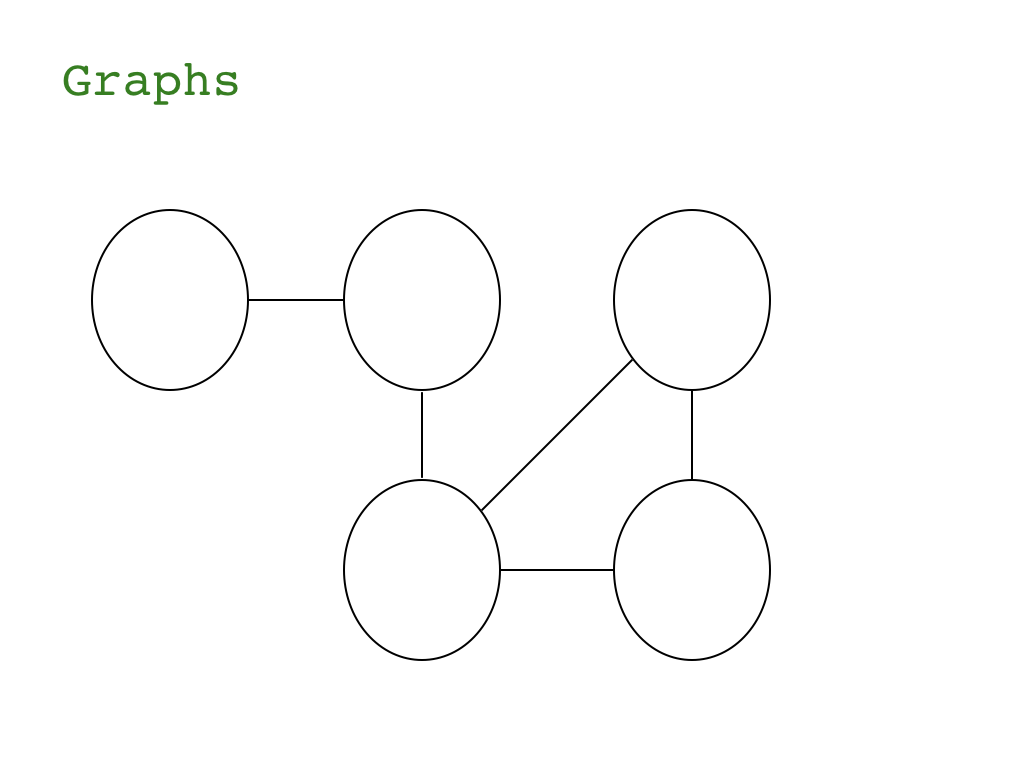
"## Network Graphs\n",
"\n",
"Basis understanding of Network Analyis using R"
]
},
{
"cell_type": "markdown",
"metadata": {},
"source": [
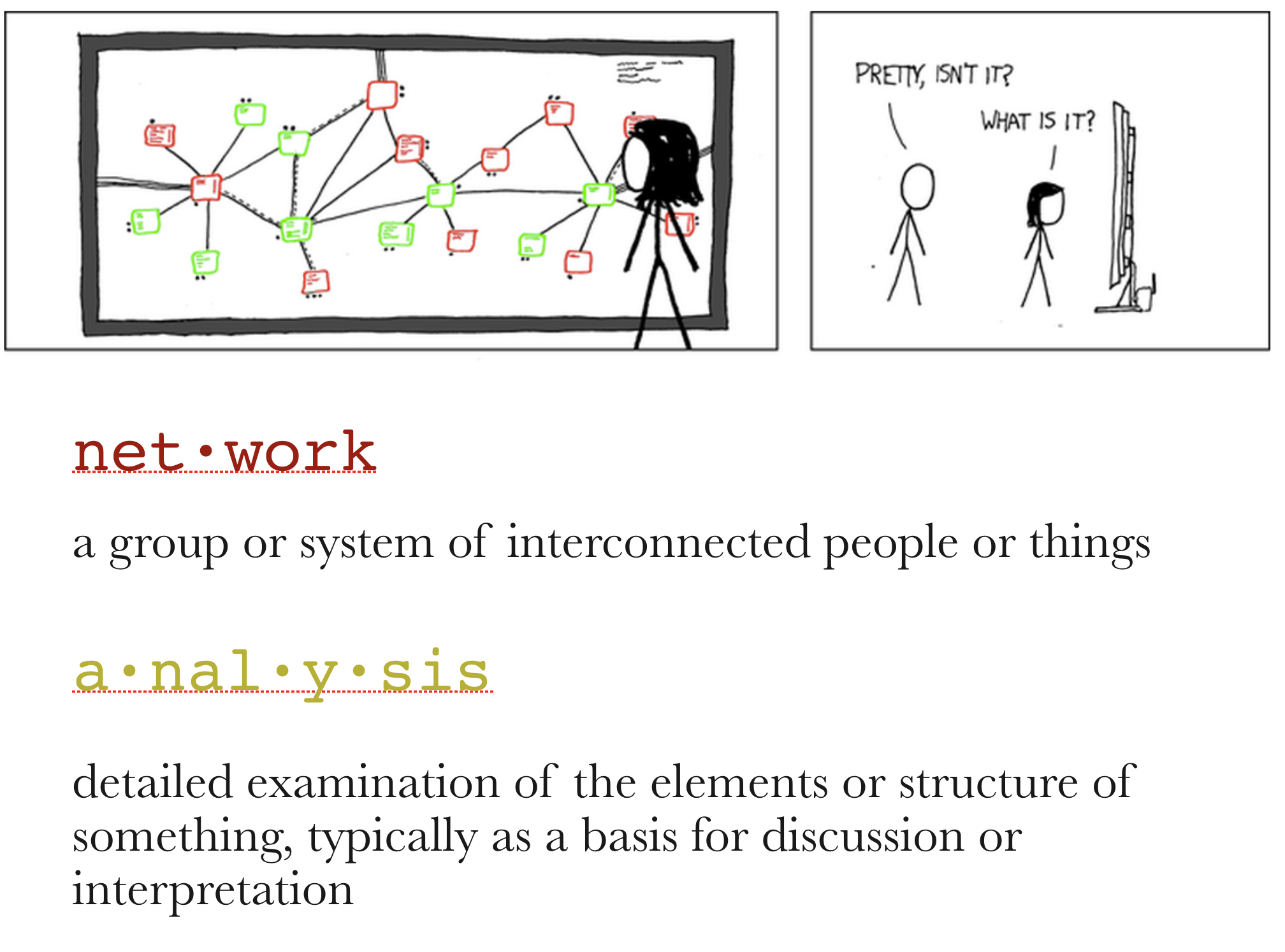
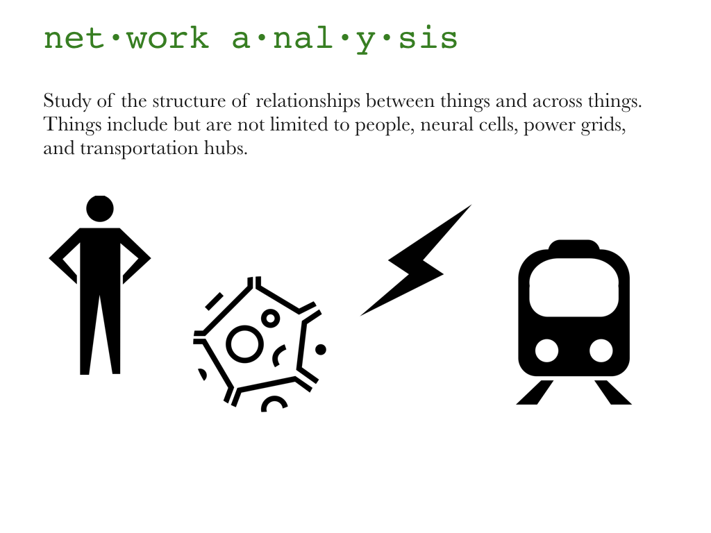
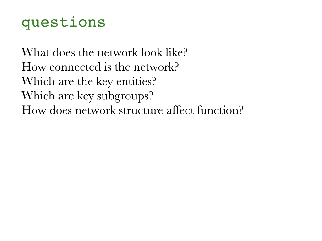
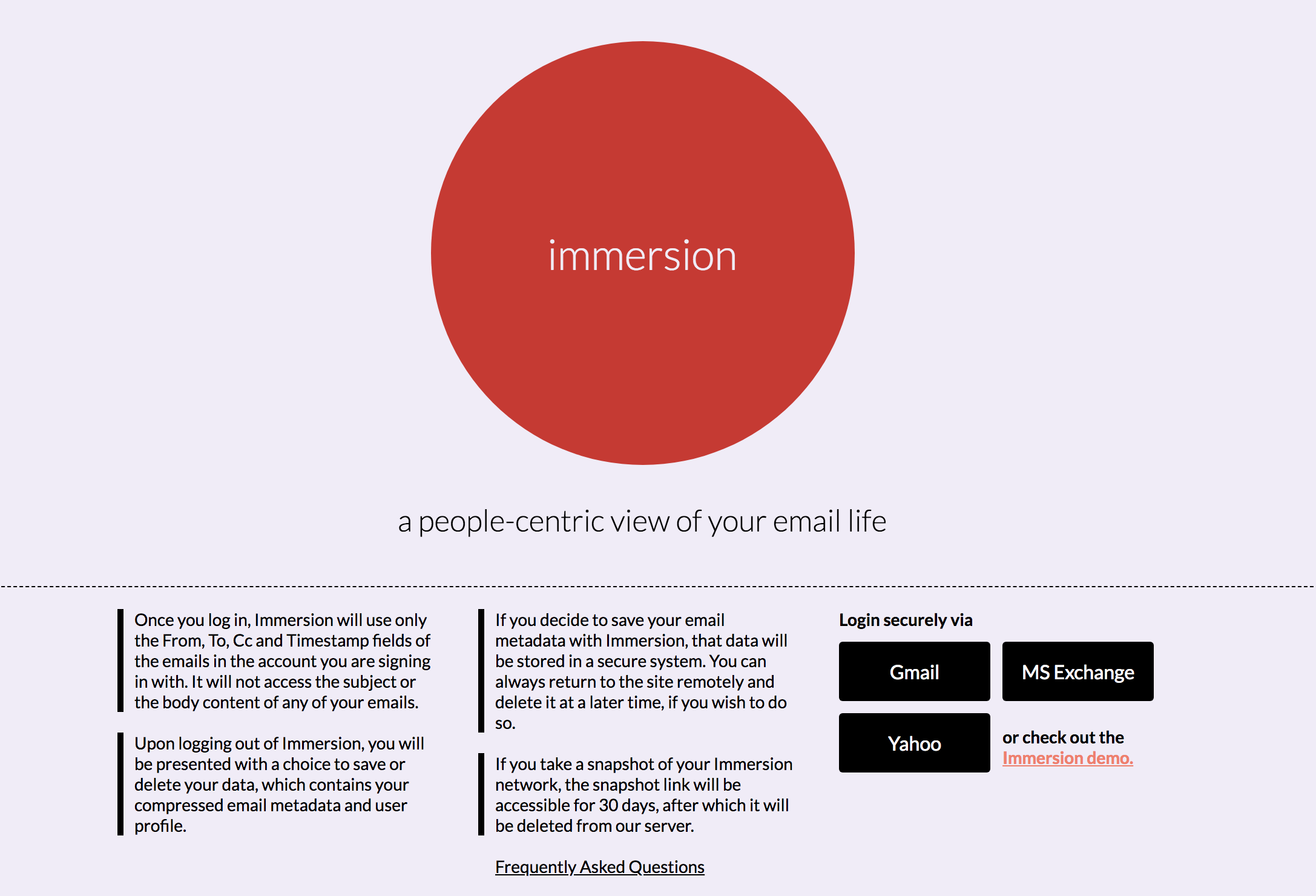
"### Intro\n",
"\n",
"\n",
"\n",
"\n",
"\n",
"\n",
"\n",
"\n",
"\n",
"\n",
"\n",
"https://immersion.media.mit.edu/demo\n",
"\n",
"\n",
"\n",
"\n",
"\n",
"\n",
"\n",
"\n",
"\n",
"\n"
]
},
{
"cell_type": "markdown",
"metadata": {},
"source": [
"### Data format, size, and preparation\n",
"In this tutorial, we will work primarily with two small example data sets. Both contain data about media organizations. One involves a network of hyperlinks and mentions among news sources. The second is a network of links between media venues and consumers. While the example data used here is small, many of the ideas behind the visualizations we will generate apply to medium and large-scale networks. This is also the reason why we will rarely use certain visual properties such as the shape of the node symbols: those are impossible to distinguish in larger graph maps. In fact, when drawing very big networks we may even want to hide the network edges, and focus on identifying and visualizing communities of nodes. At this point, the size of the networks you can visualize in R is limited mainly by the RAM of your machine. One thing to emphasize though is that in many cases, visualizing larger networks as giant hairballs is less helpful than providing charts that show key characteristics of the graph.\n",
"\n",
"First we need load some packages that we need:\n"
]
},
{
"cell_type": "code",
"execution_count": null,
"metadata": {},
"outputs": [],
"source": [
"library(igraph)\n",
"library(network) \n",
"library(sna)\n",
"library(ndtv)"
]
},
{
"cell_type": "markdown",
"metadata": {},
"source": [
"#### DATASET 1: edgelist\n",
"The first data set we are going to work with consists of two files, “Media-Example-NODES.csv” and “Media-Example-EDGES.csv”"
]
},
{
"cell_type": "code",
"execution_count": null,
"metadata": {},
"outputs": [],
"source": [
"nodes <- read.csv(\"dataJune14th/Dataset1-Media-Example-NODES.csv\", header=T, as.is=T)\n",
"links <- read.csv(\"dataJune14th/Dataset1-Media-Example-EDGES.csv\", header=T, as.is=T)"
]
},
{
"cell_type": "code",
"execution_count": null,
"metadata": {},
"outputs": [],
"source": [
"#Let's look at the data\n",
"head(nodes)\n",
"head(links)\n",
"nrow(nodes); length(unique(nodes$id))\n",
"nrow(links); nrow(unique(links[,c(\"from\", \"to\")]))"
]
},
{
"cell_type": "code",
"execution_count": null,
"metadata": {},
"outputs": [],
"source": [
"links <- aggregate(links[,3], links[,-3], sum)\n",
"links <- links[order(links$from, links$to),]\n",
"colnames(links)[4] <- \"weight\"\n",
"rownames(links) <- NULL"
]
},
{
"cell_type": "code",
"execution_count": null,
"metadata": {},
"outputs": [],
"source": [
"# Dataset 2\n",
"nodes2 <- read.csv(\"dataJune14th/Dataset2-Media-User-Example-NODES.csv\", header=T, as.is=T)\n",
"links2 <- read.csv(\"dataJune14th/Dataset2-Media-User-Example-EDGES.csv\", header=T, row.names=1)"
]
},
{
"cell_type": "code",
"execution_count": null,
"metadata": {},
"outputs": [],
"source": [
"#Examine\n",
"head(nodes2)\n",
"head(links2)"
]
},
{
"cell_type": "code",
"execution_count": null,
"metadata": {},
"outputs": [],
"source": [
"# We can see that links2 is an adjacency matrix for a two-mode network:\n",
"\n",
"\n",
"links2 <- as.matrix(links2)\n",
"dim(links2)\n",
"dim(nodes2)"
]
},
{
"cell_type": "markdown",
"metadata": {},
"source": [
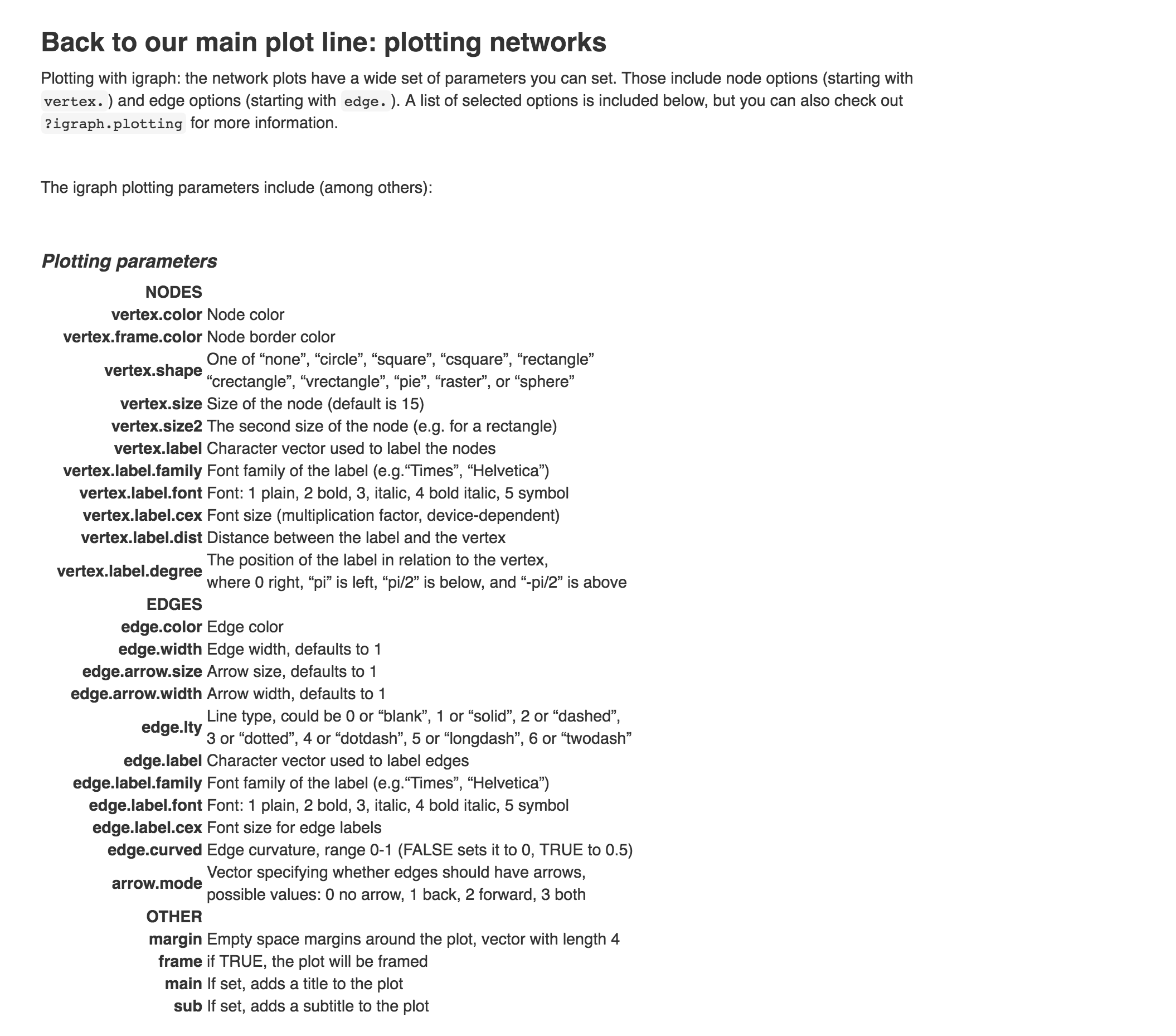
"#### Network visualization: first steps with igraph\n",
"We start by converting the raw data to an igraph network object. Here we use igraph’s graph.data.frame function, which takes two data frames: d and vertices.\n",
"\n",
"* d describes the edges of the network. Its first two columns are the IDs of the source and the target node for each edge. The following columns are edge attributes (weight, type, label, or anything else).\n",
"* vertices starts with a column of node IDs. Any following columns are interpreted as node attributes."
]
},
{
"cell_type": "code",
"execution_count": null,
"metadata": {},
"outputs": [],
"source": [
"\n",
"\n",
"net <- graph.data.frame(links, nodes, directed=T)\n",
"net"
]
},
{
"cell_type": "markdown",
"metadata": {},
"source": [
"The description of an igraph object starts with four letters:\n",
"\n",
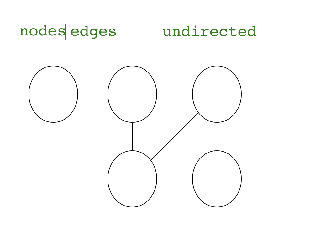
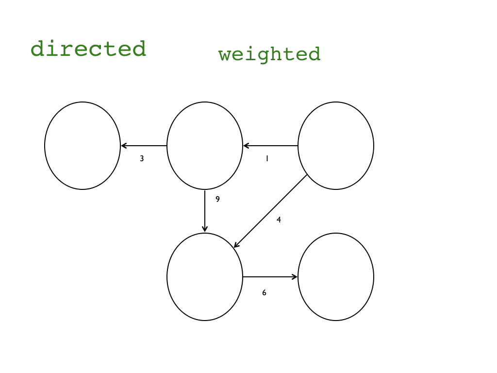
"1. D or U, for a directed or undirected graph\n",
"2. N for a named graph (where nodes have a name attribute)\n",
"3. W for a weighted graph (where edges have a weight attribute)\n",
"4. B for a bipartite (two-mode) graph (where nodes have a type attribute)\n",
"\n",
"The two numbers that follow (17 49) refer to the number of nodes and edges in the graph. The description also lists node & edge attributes, for example:\n",
"\n",
"* (g/c) - graph-level character attribute\n",
"* (v/c) - vertex-level character attribute\n",
"* (e/n) - edge-level numeric attribute\n",
"\n",
"We also have easy access to nodes, edges, and their attributes with:"
]
},
{
"cell_type": "code",
"execution_count": null,
"metadata": {},
"outputs": [],
"source": [
"E(net) # The edges of the \"net\" object\n",
"V(net) # The vertices of the \"net\" object\n",
"E(net)$type # Edge attribute \"type\"\n",
"V(net)$media # Vertex attribute \"media\"\n",
"\n",
"# You can also manipulate the network matrix directly:\n",
"net[1,]\n",
"net[5,7]"
]
},
{
"cell_type": "markdown",
"metadata": {},
"source": [
"First plot ..."
]
},
{
"cell_type": "code",
"execution_count": null,
"metadata": {},
"outputs": [],
"source": [
"plot(net) # not a pretty picture!"
]
},
{
"cell_type": "code",
"execution_count": null,
"metadata": {},
"outputs": [],
"source": [
"#That doesn’t look very good. Let’s start fixing things by removing the loops in the graph.\n",
"net <- simplify(net, remove.multiple = F, remove.loops = T) "
]
},
{
"cell_type": "markdown",
"metadata": {},
"source": [
"You might notice that could have used simplify to combine multiple edges by summing their weights with a command like simplify(net, edge.attr.comb=list(Weight=\"sum\",\"ignore\")). The problem is that this would also combine multiple edge types (in our data: “hyperlinks” and “mentions”).\n",
"\n",
"Let’s and reduce the arrow size and remove the labels (we do that by setting them to NA):"
]
},
{
"cell_type": "code",
"execution_count": null,
"metadata": {},
"outputs": [],
"source": [
"plot(net, edge.arrow.size=.4,vertex.label=NA)"
]
},
{
"cell_type": "markdown",
"metadata": {},
"source": [
"#### A brief detour I: Colors in R plots\n",
"Colors are pretty, but more importantly they help people differentiate between types of objects, or levels of an attribute. In most R functions, you can use named colors, hex, or RGB values. In the simple base R plot chart below, x and y are the point coordinates, pch is the point symbol shape, cex is the point size, and col is the color. To see the parameters for plotting in base R, check out ?par"
]
},
{
"cell_type": "code",
"execution_count": null,
"metadata": {},
"outputs": [],
"source": [
"plot(x=1:10, y=rep(5,10), pch=19, cex=3, col=\"dark red\")\n",
"points(x=1:10, y=rep(6, 10), pch=19, cex=3, col=\"557799\")\n",
"points(x=1:10, y=rep(4, 10), pch=19, cex=3, col=rgb(.25, .5, .3))"
]
},
{
"cell_type": "code",
"execution_count": null,
"metadata": {},
"outputs": [],
"source": [
"#You may notice that RGB here ranges from 0 to 1. While this is the R default, \n",
"#you can also set it for to the 0-255 range using something \n",
"#like rgb(10, 100, 100, maxColorValue=255).\n",
"\n",
"# We can set the opacity/transparency of an element using the parameter alpha (range 0-1):\n",
"plot(x=1:5, y=rep(5,5), pch=19, cex=12, col=rgb(.25, .5, .3, alpha=.5), xlim=c(0,6)) "
]
},
{
"cell_type": "code",
"execution_count": null,
"metadata": {},
"outputs": [],
"source": [
"#If we have a hex color representation, we can set the transparency alpha \n",
"#using adjustcolor from package grDevices. \n",
"#For fun, let’s also set the plot background to gray using \n",
"#the par() function for graphical parameters.\n",
"\n",
"col.tr <- grDevices::adjustcolor(\"557799\", alpha=0.7)\n",
"plot(x=1:5, y=rep(5,5), pch=19, cex=12, col=col.tr, xlim=c(0,6)) "
]
},
{
"cell_type": "code",
"execution_count": null,
"metadata": {},
"outputs": [],
"source": [
"colors() # List all named colors\n",
"grep(\"blue\", colors(), value=T) # Colors that have \"blue\" in the name"
]
},
{
"cell_type": "code",
"execution_count": null,
"metadata": {},
"outputs": [],
"source": [
"pal1 <- heat.colors(5, alpha=1) # 5 colors from the heat palette, opaque\n",
"pal2 <- rainbow(5, alpha=.5) # 5 colors from the heat palette, transparent\n",
"plot(x=1:10, y=1:10, pch=19, cex=5, col=pal1)"
]
},
{
"cell_type": "code",
"execution_count": null,
"metadata": {},
"outputs": [],
"source": [
"plot(x=1:10, y=1:10, pch=19, cex=5, col=pal2)"
]
},
{
"cell_type": "code",
"execution_count": null,
"metadata": {},
"outputs": [],
"source": [
"palf <- colorRampPalette(c(\"gray80\", \"dark red\")) \n",
"plot(x=10:1, y=1:10, pch=19, cex=5, col=palf(10)) "
]
},
{
"cell_type": "code",
"execution_count": null,
"metadata": {},
"outputs": [],
"source": [
"palf <- colorRampPalette(c(rgb(1,1,1, .2),rgb(.8,0,0, .7)), alpha=TRUE)\n",
"plot(x=10:1, y=1:10, pch=19, cex=5, col=palf(10)) "
]
},
{
"cell_type": "code",
"execution_count": null,
"metadata": {},
"outputs": [],
"source": [
"# If you don't have R ColorBrewer already, you will need to install it:\n",
"install.packages(\"RColorBrewer\")\n",
"library(RColorBrewer)\n",
"display.brewer.all()"
]
},
{
"cell_type": "code",
"execution_count": null,
"metadata": {},
"outputs": [],
"source": [
"display.brewer.pal(8, \"Set3\")"
]
},
{
"cell_type": "code",
"execution_count": null,
"metadata": {},
"outputs": [],
"source": [
"display.brewer.pal(8, \"Spectral\")"
]
},
{
"cell_type": "code",
"execution_count": null,
"metadata": {},
"outputs": [],
"source": [
"display.brewer.pal(8, \"Blues\")"
]
},
{
"cell_type": "code",
"execution_count": null,
"metadata": {},
"outputs": [],
"source": [
"pal3 <- brewer.pal(10, \"Set3\") \n",
"plot(x=10:1, y=10:1, pch=19, cex=4, col=pal3)"
]
},
{
"cell_type": "markdown",
"metadata": {},
"source": [
""
]
},
{
"cell_type": "code",
"execution_count": null,
"metadata": {},
"outputs": [],
"source": [
"# Plot with curved edges (edge.curved=.1) and reduce arrow size:\n",
"plot(net, edge.arrow.size=.4, edge.curved=.1)"
]
},
{
"cell_type": "code",
"execution_count": null,
"metadata": {},
"outputs": [],
"source": [
"# Set edge color to light gray, the node & border color to orange \n",
"# Replace the vertex label with the node names stored in \"media\"\n",
"plot(net, edge.arrow.size=.2, edge.color=\"orange\",\n",
" vertex.color=\"orange\", vertex.frame.color=\"#ffffff\",\n",
" vertex.label=V(net)$media, vertex.label.color=\"black\")"
]
},
{
"cell_type": "code",
"execution_count": null,
"metadata": {},
"outputs": [],
"source": [
"# Generate colors base on media type:\n",
"colrs <- c(\"gray50\", \"tomato\", \"gold\")\n",
"V(net)$color <- colrs[V(net)$media.type]\n",
"\n",
"# Compute node degrees (#links) and use that to set node size:\n",
"deg <- igraph::degree(net, mode=\"all\")\n",
"V(net)$size <- deg*3\n",
"# We could also use the audience size value:\n",
"V(net)$size <- V(net)$audience.size*0.6\n",
"\n",
"# The labels are currently node IDs.\n",
"# Setting them to NA will render no labels:\n",
"V(net)$label <- NA\n",
"\n",
"# Set edge width based on weight:\n",
"E(net)$width <- E(net)$weight/6\n",
"\n",
"#change arrow size and edge color:\n",
"E(net)$arrow.size <- .2\n",
"E(net)$edge.color <- \"gray80\"\n",
"E(net)$width <- 1+E(net)$weight/12\n",
"plot(net)"
]
},
{
"cell_type": "code",
"execution_count": null,
"metadata": {},
"outputs": [],
"source": [
"plot(net, edge.color=\"orange\", vertex.color=\"gray50\") "
]
},
{
"cell_type": "code",
"execution_count": null,
"metadata": {},
"outputs": [],
"source": [
"plot(net) \n",
"legend(x=-1.5, y=-1.1, c(\"Newspaper\",\"Television\", \"Online News\"), pch=21,\n",
" col=\"#777777\", pt.bg=colrs, pt.cex=2, cex=.8, bty=\"n\", ncol=1)"
]
},
{
"cell_type": "code",
"execution_count": null,
"metadata": {},
"outputs": [],
"source": [
"plot(net, vertex.shape=\"none\", vertex.label=V(net)$media, \n",
" vertex.label.font=2, vertex.label.color=\"gray40\",\n",
" vertex.label.cex=.7, edge.color=\"gray85\")"
]
},
{
"cell_type": "code",
"execution_count": null,
"metadata": {},
"outputs": [],
"source": [
"edge.start <- igraph::get.edges(net, 1:ecount(net))[,1]\n",
"edge.col <- V(net)$color[edge.start]\n",
"\n",
"plot(net, edge.color=edge.col, edge.curved=.1) "
]
},
{
"cell_type": "code",
"execution_count": null,
"metadata": {},
"outputs": [],
"source": [
"net.bg <- barabasi.game(80) \n",
"V(net.bg)$frame.color <- \"white\"\n",
"V(net.bg)$color <- \"orange\"\n",
"V(net.bg)$label <- \"\" \n",
"V(net.bg)$size <- 10\n",
"E(net.bg)$arrow.mode <- 0\n",
"plot(net.bg)"
]
},
{
"cell_type": "code",
"execution_count": null,
"metadata": {},
"outputs": [],
"source": [
"plot(net.bg, layout=layout.random)"
]
},
{
"cell_type": "code",
"execution_count": null,
"metadata": {},
"outputs": [],
"source": [
"l <- layout.circle(net.bg)\n",
"plot(net.bg, layout=l)"
]
},
{
"cell_type": "code",
"execution_count": null,
"metadata": {},
"outputs": [],
"source": [
"l <- matrix(c(1:vcount(net.bg), c(1, vcount(net.bg):2)), vcount(net.bg), 2)\n",
"plot(net.bg, layout=l)"
]
},
{
"cell_type": "code",
"execution_count": null,
"metadata": {},
"outputs": [],
"source": [
"l <- layout.random(net.bg)\n",
"plot(net.bg, layout=l)"
]
},
{
"cell_type": "code",
"execution_count": null,
"metadata": {},
"outputs": [],
"source": [
"# 3D sphere layout\n",
"l <- layout.sphere(net.bg)\n",
"plot(net.bg, layout=l)"
]
},
{
"cell_type": "code",
"execution_count": null,
"metadata": {},
"outputs": [],
"source": [
"l <- layout.fruchterman.reingold(net.bg, repulserad=vcount(net.bg)^3, \n",
" area=vcount(net.bg)^2.4)\n",
"par(mfrow=c(1,2), mar=c(0,0,0,0)) # plot two figures - 1 row, 2 columns\n",
"plot(net.bg, layout=layout.fruchterman.reingold)\n",
"plot(net.bg, layout=l)"
]
},
{
"cell_type": "code",
"execution_count": null,
"metadata": {},
"outputs": [],
"source": [
"dev.off() # shut off the graphic device to clear the two-figure configuration."
]
},
{
"cell_type": "code",
"execution_count": null,
"metadata": {},
"outputs": [],
"source": [
"l <- layout.kamada.kawai(net.bg)\n",
"plot(net.bg, layout=l)\n",
"\n",
"l <- layout.spring(net.bg, mass=.5)\n",
"plot(net.bg, layout=l)"
]
},
{
"cell_type": "code",
"execution_count": null,
"metadata": {},
"outputs": [],
"source": [
"plot(net.bg, layout=layout.lgl)"
]
},
{
"cell_type": "code",
"execution_count": null,
"metadata": {},
"outputs": [],
"source": [
"l <- layout.fruchterman.reingold(net.bg)\n",
"l <- layout.norm(l, ymin=-1, ymax=1, xmin=-1, xmax=1)\n",
"\n",
"par(mfrow=c(2,2), mar=c(0,0,0,0))\n",
"plot(net.bg, rescale=F, layout=l*0.4)\n",
"plot(net.bg, rescale=F, layout=l*0.6)\n",
"plot(net.bg, rescale=F, layout=l*0.8)\n",
"plot(net.bg, rescale=F, layout=l*1.0)"
]
},
{
"cell_type": "code",
"execution_count": null,
"metadata": {},
"outputs": [],
"source": [
"layouts <- grep(\"^layout\\\\.\", ls(\"package:igraph\"), value=TRUE) \n",
"# Remove layouts that do not apply to our graph.\n",
"layouts <- layouts[!grepl(\"bipartite|merge|norm|sugiyama\", layouts)]\n",
"\n",
"par(mfrow=c(3,3))\n",
"\n",
"for (layout in layouts) {\n",
" print(layout)\n",
" l <- do.call(layout, list(net)) \n",
" plot(net, edge.arrow.mode=0, layout=l, main=layout) }\n",
"\n",
"dev.off()"
]
},
{
"cell_type": "code",
"execution_count": null,
"metadata": {},
"outputs": [],
"source": [
"hist(links$weight)\n",
"mean(links$weight)\n",
"sd(links$weight)"
]
},
{
"cell_type": "code",
"execution_count": null,
"metadata": {},
"outputs": [],
"source": [
"cut.off <- mean(links$weight) \n",
"net.sp <- igraph::delete.edges(net, E(net)[weight