# geoconformal
Main contributors
[](https://opensource.org/licenses/MIT)
[](https://www.python.org/downloads/)
[](https://pypi.org/project/geoconformal/)
[](https://pepy.tech/project/geoconformal)
[](https://pypi.org/project/geoconformal/)
[](https://github.com/pengtum/geoconformal)
[](https://spatialuncertaintyviz-production.up.railway.app)
**Model-agnostic uncertainty quantification for geospatial prediction.**
`geoconformal` attaches a prediction interval to any spatial model (XGBoost, Random Forest, neural nets, …) **without retraining it** — and tells you **how much to trust each interval**.
> **🌐 Try it live — [interactive demo](https://spatialuncertaintyviz-production.up.railway.app).** Pick a dataset, a base model, and a conformal-prediction method, then explore coverage, uncertainty, intervals, posterior and effective-sample-size views right in your browser — no install.
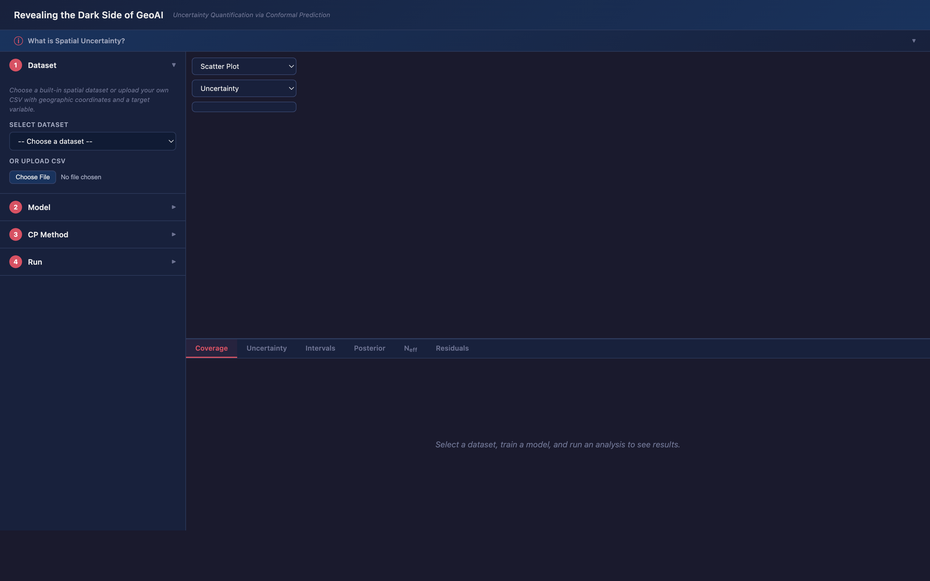
▶ Open the live app — “Revealing the Dark Side of GeoAI”
### Why this matters
A map of predictions is only actionable if it carries a reliable statement of uncertainty. For spatial data that uncertainty has **two levels**, and most tools address only the first:
1. **How uncertain is the prediction at each location?** Model error is *spatially non-stationary* — one global ± error bar overstates confidence in hard regions and wastes it in easy ones. **GeoCP / GeoSIMCP** give a *location-specific* interval by weighting calibration errors toward each test point.
2. **How much can you trust that interval itself?** Each local interval is estimated from whatever calibration data happens to lie nearby — in data-sparse areas it rests on a handful of points, yet on a map it looks just as authoritative as one backed by hundreds. **GeoBCP** adds a *posterior over the interval* — **uncertainty about the uncertainty** — so "wide because genuinely uncertain" is distinguishable from "wide/narrow but barely supported."
Skipping level 2 is how a "90%" map quietly under-covers exactly where data is thin — and where decisions are riskiest.
### Two dimensions
The methods sit on **two independent axes** — choose one option on each:
**Dimension 1 — how the uncertainty is *localized* (the weighting).** GeoCP and GeoSIMCP are parallel choices:
- **GeoCP** — geographic distance only (Tobler: nearby ≈ similar).
- **GeoSIMCP** — geographic distance **+ feature similarity**, for nonstationary processes where neighbours can belong to different regimes.
**Dimension 2 — how confident you are *in that uncertainty*.**
- **Point estimate** — one interval per location.
- **GeoBCP (Bayesian)** — a *posterior* over each location's interval: its width **plus** a reliability readout (posterior spread, local effective sample size, probability the interval is uninformative). This is the *uncertainty on the uncertainty*.
| | **Point estimate** → the interval | **GeoBCP** (Bayesian) → interval **+ its reliability** |
|---|---|---|
| **GeoCP** — geographic | `GeoConformalSpatialRegression` | `GeoConformalRegressor(..., bayesian=True)` |
| **GeoSIMCP** — geo + feature | `GeoSIMConformalSpatialRegression` | engine: `GeoConformalPrediction` + `joint_geo_feature_weights` |
> A third, optional axis is **finite-sample validity**: pass `include_test_atom=True` to guarantee coverage on small / sparse calibration sets — where local data genuinely cannot certify the level the interval becomes `+∞` (an honest abstention).
New in 0.3.0. See **[Choosing a method](#choosing-a-method--applicability-guide)** for detailed guidance, and the **[GeoBCP tutorial](example/geobcp_tutorial.ipynb)** for a walkthrough of the second dimension.
## Installation
```bash
pip install geoconformal
```
Requires Python >= 3.7. Dependencies: `numpy`, `scikit-learn`, `scipy`, `pandas`, `geopandas`.
---
## Quick Start
### Step 1: Train your prediction model (any model works)
```python
from sklearn.ensemble import RandomForestRegressor
model = RandomForestRegressor(n_estimators=100, random_state=42)
model.fit(X_train, y_train)
```
### Step 2: Quantify uncertainty with GeoCP
```python
from geoconformal import GeoConformalSpatialRegression
geo_cp = GeoConformalSpatialRegression(
predict_f=model.predict, # your model's predict function
bandwidth=2.0, # kernel bandwidth
miscoverage_level=0.1, # 0.1 = 90% prediction interval
coord_calib=coords_calib, # calibration set coordinates, shape (n, 2)
coord_test=coords_test, # test set coordinates, shape (m, 2)
X_calib=X_calib, # calibration features
y_calib=y_calib, # calibration true values
X_test=X_test, # test features
y_test=y_test, # test true values
)
results = geo_cp.analyze()
```
That's it. `results` contains everything you need.
---
## Understanding the Concepts
### What is Conformal Prediction?
Traditional machine learning models give you a **single predicted value** (e.g., "the house price is $500K"). But how confident is that prediction? Conformal prediction answers this by providing a **prediction interval** (e.g., "the house price is between $450K and $550K, with 90% confidence").
The figure below illustrates the workflow. **(a) Standard Conformal Prediction** treats all calibration residuals equally to compute a single global quantile. **(b) Weighted Conformal Prediction (GeoCP/GeoSIMCP)** assigns location-specific weights so each test point gets its own prediction interval.
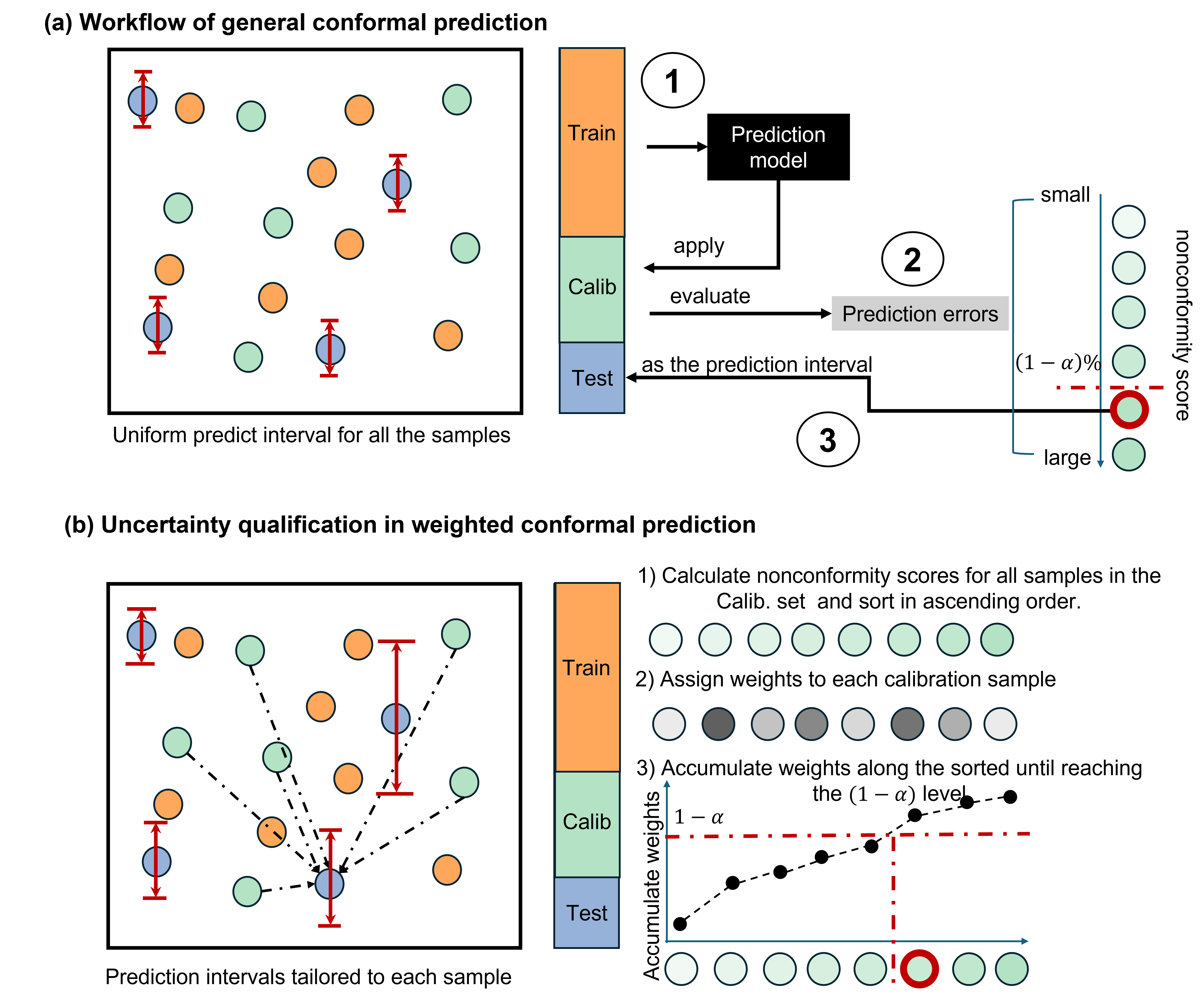
The key idea:
1. **Train** your model on training data
2. **Calibrate**: compute residuals (prediction errors) on a held-out calibration set
3. **Quantify**: use the **weighted** distribution of residuals to build intervals for new test points
### What makes GeoCP special?
Standard conformal prediction treats all calibration residuals equally. But in spatial data, **nearby locations tend to behave similarly** (Tobler's First Law of Geography). GeoCP assigns **higher weights to geographically closer** calibration points when computing the prediction interval for each test location.
This means each test point gets its own **location-specific** prediction interval, reflecting the local uncertainty structure.
### What makes GeoSIMCP different from GeoCP?
GeoCP only considers **geographic distance**. But sometimes nearby locations have very different characteristics. For example, two adjacent properties might be in different land-use zones (residential vs. commercial), leading to very different price distributions despite being close in space.
The figure below shows the key difference. In the left panel (**GeoCP**), the hollow test point is weighted by geographic distance alone, so calibration samples from a different spatial process (pink region) receive high weights simply because they are nearby. In the right panel (**GeoSIMCP**), feature similarity is also considered, so calibration samples that are process-consistent (blue region) contribute more, even if they are farther away.
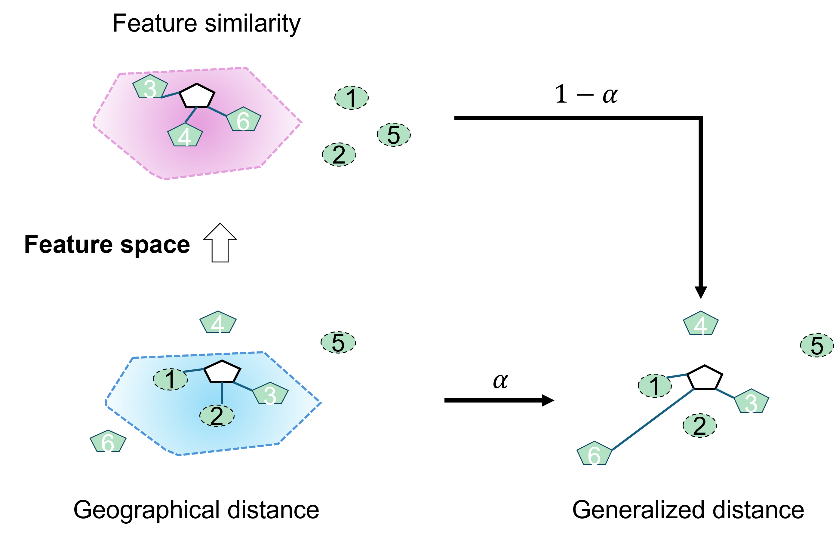
GeoSIMCP measures similarity using **both geographic distance AND feature similarity**:
```
d_joint = sqrt( lambda * d_geo^2 + (1 - lambda) * d_feat^2 )
```
- When `lambda = 1.0`: only geographic distance matters (equivalent to GeoCP)
- When `lambda = 0.0`: only feature similarity matters
- When `0 < lambda < 1`: both contribute
### Full Workflow of GeoSIMCP
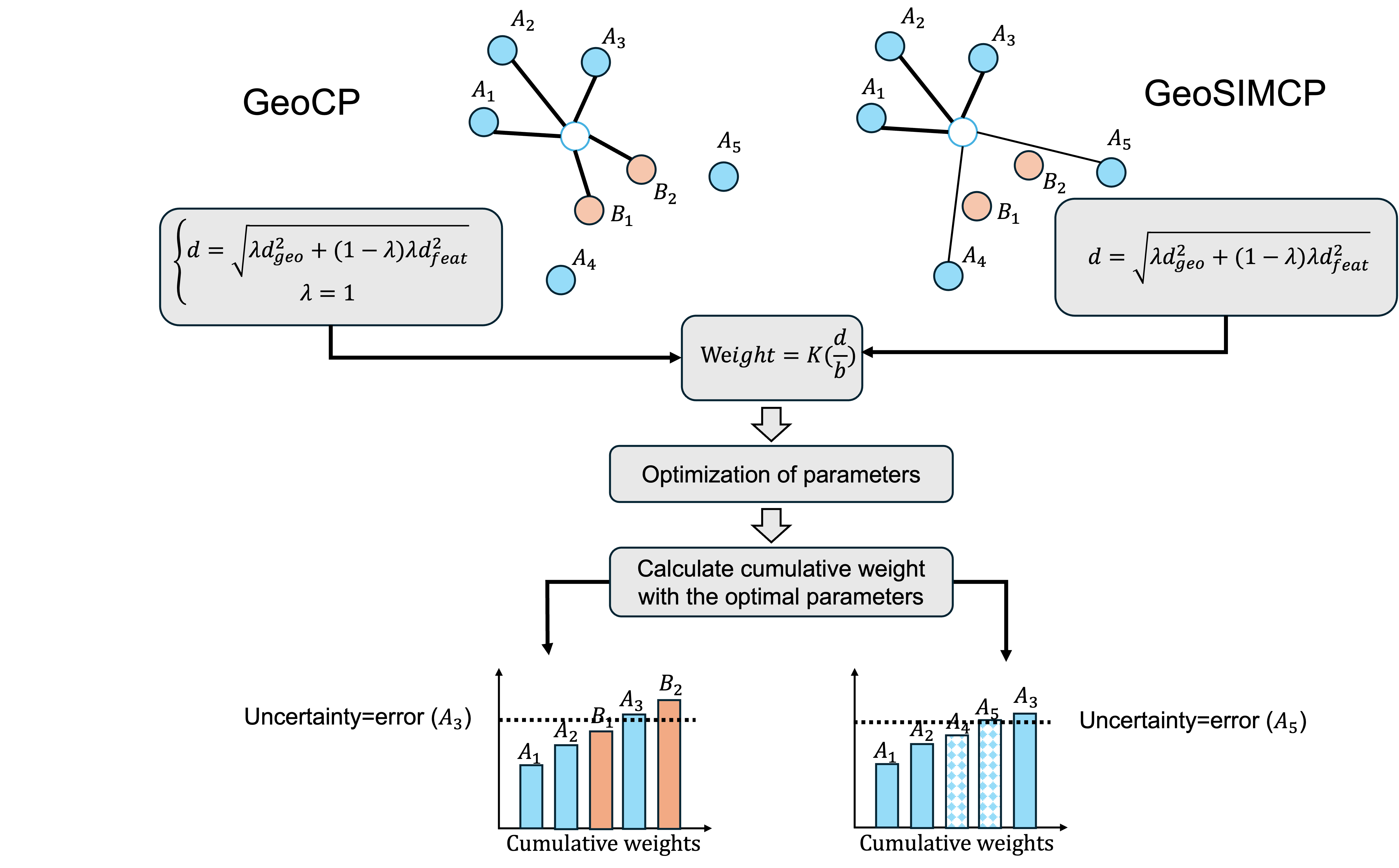
The figure below shows the complete GeoSIMCP pipeline. For GeoCP (left), only the bandwidth parameter `b` is optimized. For GeoSIMCP (right), both `b` and the trade-off parameter `lambda` are jointly optimized via grid search to minimize the interval score while maintaining valid coverage.
---
## Example Notebook
A complete step-by-step tutorial is available at **[`example/geoconformal_tutorial.ipynb`](example/geoconformal_tutorial.ipynb)**, covering:
- GeoCP and GeoSIMCP usage with the Seattle housing dataset
- Hyperparameter tuning (grid search with visualization)
- Spatial mapping of predictions and uncertainty
---
## Data Preparation
The package expects your data to be split into four sets:
```
Full Dataset
|-- Training set (e.g., 70%) --> used to train your prediction model
|-- Calibration set (e.g., 10%) --> used by geoconformal to compute residuals
|-- Validation set (e.g., 10%) --> used to tune hyperparameters (bandwidth, lambda)
|-- Test set (e.g., 10%) --> final evaluation of uncertainty estimates
```
**Important**: Hyperparameters (bandwidth, lambda) should be tuned on the **validation set**, not the test set. The test set should only be used for final evaluation to avoid data leakage.
Example split:
```python
from sklearn.model_selection import train_test_split
# First split: 70% train, 30% remaining
X_train, X_remain, y_train, y_remain, coords_train, coords_remain = \
train_test_split(X, y, coords, test_size=0.3, random_state=42)
# Second split: remaining into calib (1/3), val (1/3), test (1/3)
X_calib, X_temp, y_calib, y_temp, coords_calib, coords_temp = \
train_test_split(X_remain, y_remain, coords_remain, test_size=2/3, random_state=42)
X_val, X_test, y_val, y_test, coords_val, coords_test = \
train_test_split(X_temp, y_temp, coords_temp, test_size=0.5, random_state=42)
```
---
## API Reference
### GeoConformalSpatialRegression (GeoCP)
Uses **geographic distance only** to weight calibration residuals.
```python
from geoconformal import GeoConformalSpatialRegression
geo_cp = GeoConformalSpatialRegression(
predict_f, # Callable: your model's predict function
nonconformity_score_f, # Callable, optional: custom score function
miscoverage_level, # float: e.g. 0.1 for 90% intervals
bandwidth, # float: Gaussian kernel bandwidth
coord_calib, # array (n, 2): calibration coordinates
coord_test, # array (m, 2): test coordinates
X_calib, # array (n, p): calibration features
y_calib, # array (n,): calibration true values
X_test, # array (m, p): test features
y_test, # array (m,): test true values
)
```
### GeoSIMConformalSpatialRegression (GeoSIMCP)
Uses **geographic distance + feature similarity** jointly. All GeoCP parameters apply, plus:
```python
from geoconformal import GeoSIMConformalSpatialRegression
geo_simcp = GeoSIMConformalSpatialRegression(
predict_f,
miscoverage_level=0.1,
bandwidth=2.0,
coord_calib=coords_calib,
coord_test=coords_test,
X_calib=X_calib,
y_calib=y_calib,
X_test=X_test,
y_test=y_test,
# --- GeoSIMCP-specific parameters ---
lambda_weight=0.5, # float in [0, 1], default 1.0
distance_metric='euclidean', # 'euclidean' or 'mnd'
standardize_weights=True, # z-score normalize features for distance
X_calib_weight=None, # optional: separate features for distance
X_test_weight=None, # optional: separate features for distance
)
```
### Parameter Details
#### `predict_f` (required)
Your model's prediction function. Must accept a feature matrix and return an array of predictions.
```python
# scikit-learn models
predict_f = model.predict
# Custom function
def my_predict(X):
return X @ weights + bias
predict_f = my_predict
```
#### `miscoverage_level` (default: 0.1)
Controls the confidence level of prediction intervals.
| Value | Confidence Level | Interval Width |
|-------|-----------------|----------------|
| 0.01 | 99% | Very wide |
| 0.05 | 95% | Wide |
| **0.1** | **90%** | **Moderate (recommended)** |
| 0.2 | 80% | Narrow |
Lower values = wider intervals = higher coverage but less informative.
#### `bandwidth`
Controls how quickly geographic influence decays with distance. Uses a **Gaussian kernel**: `w = exp(-0.5 * (d / bandwidth)^2)`.
| Bandwidth | Effect |
|-----------|--------|
| Small (e.g., 0.1) | Only very close calibration points matter. Highly localized but potentially unstable. |
| Medium (e.g., 1-3) | Balanced local sensitivity. **Good starting point.** |
| Large (e.g., 5+) | Most calibration points contribute. Smooth but may oversmooth local patterns. |
**Tip**: Use grid search to find the optimal bandwidth. Start with a range like `[0.1, 0.5, 1.0, 2.0, 3.0, 5.0]`.
#### `lambda_weight` (GeoSIMCP only, default: 1.0)
Trade-off between geographic and feature distance.
| Value | Behavior | Use when... |
|-------|----------|-------------|
| 1.0 | Pure geographic distance (= GeoCP) | Spatial interpolation, no features |
| 0.7 | Mostly geographic, some feature | Strong spatial structure with mild heterogeneity |
| 0.5 | Equal weight | Balanced spatial and feature effects |
| 0.3 | Mostly feature, some geographic | Strong feature-driven heterogeneity |
| 0.0 | Pure feature distance | Uncertainty fully determined by feature similarity |
**Tip**: Use grid search over `lambda` in `[0, 0.05, 0.1, ..., 0.95, 1.0]` together with bandwidth.
#### `distance_metric` (GeoSIMCP only, default: 'euclidean')
How feature-space distance is calculated.
- **`'euclidean'`** (EUC): Standard Euclidean distance across all feature dimensions. Works well when features contribute relatively equally.
- **`'mnd'`** (Minimum Normalized Difference): Focuses on the **single most dissimilar feature**. More robust when one dominant feature drives differences between locations (e.g., land-use type).
```python
# Euclidean distance (default)
geo_simcp = GeoSIMConformalSpatialRegression(..., distance_metric='euclidean')
# MND distance
geo_simcp = GeoSIMConformalSpatialRegression(..., distance_metric='mnd')
```
#### `standardize_weights` (GeoSIMCP only, default: True)
When `True`, features used for distance computation are z-score normalized so that all dimensions contribute equally. Only applies when `distance_metric='euclidean'`. Geographic coordinates are **never** standardized (they carry physical meaning).
#### `X_calib_weight` / `X_test_weight` (GeoSIMCP only, optional)
By default, the same features used for prediction (`X_calib`, `X_test`) are used for distance computation. Use these parameters to specify **different features** for distance weighting.
```python
# Use only land-use and elevation for distance, but all features for prediction
geo_simcp = GeoSIMConformalSpatialRegression(
...,
X_calib=X_calib_full, # all features for prediction
X_test=X_test_full,
X_calib_weight=X_calib[['landuse', 'elevation']], # subset for distance
X_test_weight=X_test[['landuse', 'elevation']],
)
```
#### `nonconformity_score_f` (optional)
Custom function to measure how "nonconforming" a prediction is. Default: absolute residual `|predicted - actual|`.
```python
# Default (absolute residual)
nonconformity_score_f = None # uses |pred - gt|
# Custom: squared residual
def squared_residual(pred, gt):
return (pred - gt) ** 2
geo_cp = GeoConformalSpatialRegression(..., nonconformity_score_f=squared_residual)
```
---
## Working with Results
The `analyze()` method returns a `GeoConformalResults` object:
```python
results = geo_cp.analyze()
# Access individual attributes
results.geo_uncertainty # array (m,): per-location uncertainty
results.uncertainty # float: global average uncertainty
results.pred # array (m,): predicted values
results.upper_bound # array (m,): upper bound of interval
results.lower_bound # array (m,): lower bound of interval
results.coverage_probability # float: proportion of test points covered
# Convert to GeoDataFrame for mapping
gdf = results.to_gpd() # GeoDataFrame with geometry column
```
### Visualization Example
```python
import matplotlib.pyplot as plt
gdf = results.to_gpd()
fig, axes = plt.subplots(1, 2, figsize=(14, 5))
# Map 1: Predictions
gdf.plot(column='pred', cmap='RdYlBu_r', legend=True, ax=axes[0])
axes[0].set_title('Predicted Values')
# Map 2: Uncertainty
gdf.plot(column='geo_uncertainty', cmap='Reds', legend=True, ax=axes[1])
axes[1].set_title('Prediction Uncertainty')
plt.tight_layout()
plt.show()
```
---
## Step-by-Step Methods
Instead of `analyze()`, you can run each step individually:
```python
geo_cp = GeoConformalSpatialRegression(...)
# Step 1: Compute uncertainty for each test location
geo_cp.predict_geoconformal_uncertainty()
# Step 2: Build prediction intervals
geo_cp.predict_confidence_interval()
# Step 3: Evaluate coverage
geo_cp.coverage_probability()
# Access results directly
print(f"Coverage: {geo_cp.coverage_proba:.3f}")
print(f"Mean uncertainty: {geo_cp.uncertainty:.3f}")
print(f"Intervals: [{geo_cp.lower_bound[0]:.2f}, {geo_cp.upper_bound[0]:.2f}]")
```
---
## Hyperparameter Tuning
### For GeoCP: tune bandwidth
Tune on the **validation set**, then evaluate on the **test set**.
```python
best_score = float('inf')
best_bw = None
for bw in [0.1, 0.5, 1.0, 2.0, 3.0, 5.0]:
geo_cp = GeoConformalSpatialRegression(
predict_f=model.predict, bandwidth=bw, miscoverage_level=0.1,
coord_calib=coords_calib, coord_test=coords_val, # validate on val set
X_calib=X_calib, y_calib=y_calib, X_test=X_val, y_test=y_val,
)
results = geo_cp.analyze()
# Interval score: width + penalty for miscoverage
width = results.upper_bound - results.lower_bound
alpha = 0.1
penalty = (2 / alpha) * (
np.maximum(results.lower_bound - y_val, 0) +
np.maximum(y_val - results.upper_bound, 0)
)
score = np.mean(width + penalty)
if results.coverage_probability >= 0.9 and score < best_score:
best_score = score
best_bw = bw
print(f"Best bandwidth: {best_bw}, interval score: {best_score:.3f}")
```
### For GeoSIMCP: tune bandwidth + lambda
```python
import numpy as np
best_score = float('inf')
best_params = None
for bw in np.linspace(0.1, 5.0, 20):
for lam in np.arange(0, 1.05, 0.05):
geo_simcp = GeoSIMConformalSpatialRegression(
predict_f=model.predict, bandwidth=bw, lambda_weight=lam,
miscoverage_level=0.1, distance_metric='euclidean',
coord_calib=coords_calib, coord_test=coords_val, # validate on val set
X_calib=X_calib, y_calib=y_calib, X_test=X_val, y_test=y_val,
)
results = geo_simcp.analyze()
width = results.upper_bound - results.lower_bound
alpha = 0.1
penalty = (2 / alpha) * (
np.maximum(results.lower_bound - y_val, 0) +
np.maximum(y_val - results.upper_bound, 0)
)
score = np.mean(width + penalty)
if results.coverage_probability >= 0.9 and score < best_score:
best_score = score
best_params = (bw, lam)
print(f"Best bandwidth: {best_params[0]:.2f}, lambda: {best_params[1]:.2f}")
```
---
## Choosing a method — applicability guide
Every method here is the same engine with different choices along three independent axes: **(1) how calibration points are weighted**, **(2) point estimate vs. Bayesian posterior**, and **(3) whether the finite-sample `+∞` test atom is included**. They target *different guarantees*, so the question is which fits your problem — not which "wins".
### Axis 1 — how should calibration points be weighted?
- **Only coordinates, or pure spatial interpolation → GeoCP** (`GeoConformalSpatialRegression`). Assumes nearby locations have similar errors (Tobler's first law). The right default when you have no informative features or the error surface is spatially smooth. *Assumption:* local stationarity in space. *Cost:* over-weights nearby points even when they belong to a different process.
- **Features available *and* the process is nonstationary → GeoSIMCP** (`GeoSIMConformalSpatialRegression`). When two nearby locations can belong to different regimes (e.g. residential vs. commercial parcels), geographic distance alone pulls in the wrong neighbors. GeoSIMCP blends geographic and feature distance via `lambda_weight` (`λ=1` → pure GeoCP, `λ=0` → pure feature similarity). Tune `λ`; if the optimum is `1.0`, the process is effectively stationary and GeoCP suffices. Use `distance_metric='mnd'` when a single dominant feature separates regimes (e.g. land-use class), `'euclidean'` when features matter roughly equally. *Cost:* an extra hyperparameter to tune.
- **The mismatch is in feature space, not geography (covariate shift) → `covariate_shift_weights`.** When calibration and deployment differ in their *feature* distribution (you calibrated on one population, deploy on another), weight by the density ratio `p_test/p_calib`. *Requires:* an estimate of that ratio.
- **You just want neighbourhood-local intervals → `knn_weights`** (localized CP, Guan 2023): each test point uses its `k` nearest calibration neighbours, no kernel bandwidth to set.
- **Baseline / no localization → `uniform_weights`** = standard split conformal prediction. Use as a reference, or when nothing justifies localizing.
### Axis 2 — do you need to know how *reliable* each interval is?
- **One interval per location is enough → point estimate** (the classes above, or `.conformalize()`). A single threshold per point.
- **You need per-location meta-uncertainty → GeoBCP** (`GeoConformalRegressor(..., bayesian=True)`). Returns a *posterior* over each location's threshold, so you can tell a wide-but-solid interval from a wide-but-unreliable one: posterior standard deviation, Kish effective sample size (how much local data supports the point), and the probability the interval is uninformative (`prob_infinite`). Use it for decision maps where interval *trustworthiness* matters. *Cost:* Monte-Carlo sampling — slower than the point estimate.
### Axis 3 — is your calibration set small, or are some test points poorly sampled?
- **Large, dense, well-covered → leave `include_test_atom=False`** (the default). Marginal coverage is already close to target and intervals stay finite. This also reproduces the behaviour published in the GeoCP / GeoSIMCP papers.
- **Small `n`, or test points far from calibration data → `include_test_atom=True`.** Adds the unobserved test residual's `+∞` atom (Tibshirani et al. 2019), guaranteeing finite-sample coverage. Where the local data genuinely cannot certify the requested level, the interval becomes `+∞` — an explicit "not enough evidence here" instead of a falsely narrow interval. Use it when under-coverage is costly and honest abstention is acceptable; **avoid it (or widen the bandwidth)** if you must return a finite interval everywhere.
### Quick decision flow
```
Only coordinates? ───────────────────── yes → GeoCP
│ no (have features)
▼
Can nearby points differ by regime? ──── yes → GeoSIMCP (tune lambda; 'mnd' if one feature dominates)
│ no no → GeoCP
▼
Calibration small / sparse? ──────────── yes → add include_test_atom=True
▼
Need per-interval reliability? ───────── yes → GeoBCP (bayesian=True)
▼
Non-spatial shift / localized / baseline?
→ covariate_shift_weights / knn_weights / uniform_weights
```
These choices **compose**: e.g. GeoSIMCP + `include_test_atom=True`, or spatial weights + Bayesian (GeoBCP). GeoCP/GeoSIMCP give spatially-varying marginal coverage; the test atom adds finite-sample validity; GeoBCP adds per-location reliability.
---
## Finite-sample-valid & Bayesian GeoCP (`geoconformal.geocp`, new in 0.3.0)
`geoconformal` is built on one engine, `GeoConformalPrediction`, which accepts any weight function and supports both a point-estimate threshold and a Bayesian posterior; the classic `GeoConformalSpatialRegression` / `GeoSIMConformalSpatialRegression` classes are convenience wrappers over it. Two capabilities of the engine are worth calling out:
- **Finite-sample correction (the `+∞` test atom)** — following Tibshirani et al. (2019), the unobserved test point contributes its own atom at `+∞` with weight `w(x)`, which restores finite-sample coverage on small / sparse calibration sets; where local support is genuinely insufficient the interval becomes `+∞` (an honest abstention rather than silent under-coverage). It is **opt-in**: pass `include_test_atom=True` to the classic classes, or use the engine / `GeoConformalRegressor`. With `uniform_weights` the engine reduces **exactly** to standard split conformal prediction.
- **GeoBCP (Bayesian)** — puts a *posterior* over each location's threshold via a weighted Dirichlet whose concentration is Kish's effective sample size, and reports an HPD interval at confidence `beta`, plus per-location diagnostics (effective sample size, posterior standard deviation, probability the interval is infinite).
### Usage
```python
from geoconformal import GeoConformalRegressor
from sklearn.ensemble import RandomForestRegressor
model = RandomForestRegressor().fit(X_train, y_train)
reg = GeoConformalRegressor(
predict_f=model.predict,
x_calib=X_calib, y_calib=y_calib, coord_calib=coords_calib,
bandwidth=0.15, miscoverage_level=0.1, # 90% target coverage
# adaptive=True, k=20, # optional k-NN adaptive bandwidth
)
# Corrected GeoCP (point-estimate threshold, finite-sample valid)
res = reg.geo_conformalize(X_test, y_test, coords_test)
print(res.coverage, res.mean_width_finite, res.frac_infinite)
# GeoBCP (Bayesian threshold posterior + HPD interval)
bres = reg.geo_conformalize(X_test, y_test, coords_test, bayesian=True, beta=0.9, num_mc=1000)
print(bres.coverage, bres.mean_n_eff, bres.summary())
```
### Diagnostics (`GeoCPResults`)
| Field / property | Meaning |
|---|---|
| `coverage` | empirical coverage on the test set |
| `lower_bound` / `upper_bound` / `uncertainty` | per-point interval and half-width |
| `frac_infinite` | fraction of points that abstained (interval = `+∞`) |
| `mean_width_finite` | mean interval width over finite (certifiable) points |
| `n_eff` *(Bayesian)* | per-point Kish effective sample size — how much local data supports the threshold |
| `posterior_std` *(Bayesian)* | per-point posterior SD of the threshold (meta-uncertainty) |
| `prob_infinite` *(Bayesian)* | posterior probability the interval is infinite |
### Advanced — arbitrary weight schemes
`GeoConformalRegressor` is a thin spatial wrapper over `GeoConformalPrediction`, which accepts any weight function from `geoconformal.geocp.weights`:
| factory | method |
|---|---|
| `spatial_kernel_weights` | GeoCP / GeoBCP (Gaussian kernel on coordinates) |
| `adaptive_spatial_weights` | adaptive-bandwidth GeoCP |
| `covariate_shift_weights` | weighted CP under covariate shift (Tibshirani 2019) |
| `knn_weights` | localized CP (Guan 2023) |
| `uniform_weights` | standard split CP |
| `rbf_feature_weights` | RBF kernel in feature space |
```python
from geoconformal import GeoConformalPrediction
from geoconformal.geocp.weights import spatial_kernel_weights
weight_fn = spatial_kernel_weights(coords_calib, bandwidth=0.15)
geo = GeoConformalPrediction(model.predict, X_calib, y_calib, weight_fn, miscoverage_level=0.1)
res = geo.conformalize(X_test, y_test, coord_test=coords_test) # point estimate
bres = geo.bayesian_conformalize(X_test, y_test, coord_test=coords_test, beta=0.9) # Bayesian
```
> **Note** — this framework is model-agnostic (NumPy in/out) and does **not** return a `GeoDataFrame`. Use it when you need finite-sample validity or threshold posteriors; use `GeoConformalSpatialRegression` / `GeoSIMConformalSpatialRegression` when you want the stateful `.analyze()` / `.to_gpd()` workflow. Self-contained finite-sample coverage checks live in [`experiments/`](experiments/).
---
## Citation
If you use this package in your research, please cite:
**GeoCP:**
```bibtex
@article{lou2025geoconformal,
title={Geoconformal prediction: a model-agnostic framework for measuring the uncertainty of spatial prediction},
author={Lou, Xiayin and Luo, Peng and Meng, Liqiu},
journal={Annals of the American Association of Geographers},
volume={115},
number={8},
pages={1971--1998},
year={2025},
publisher={Taylor \& Francis}
}
```
**GeoSIMCP:**
```bibtex
@article{luo2025geosimcp,
title={Quantifying uncertainty in spatial prediction for nonstationary spatial processes},
author={Luo, Peng},
journal={Annals of the American Association of Geographers},
year={2026}
}
```
**GeoBCP / Weighted Bayesian Conformal Prediction** (the `geoconformal.geocp` framework):
```bibtex
@article{lou2026wbcp,
title={Weighted Bayesian Conformal Prediction},
author={Lou, Xiayin and Luo, Peng},
journal={arXiv preprint arXiv:2604.06464},
year={2026}
}
```
## License
MIT License