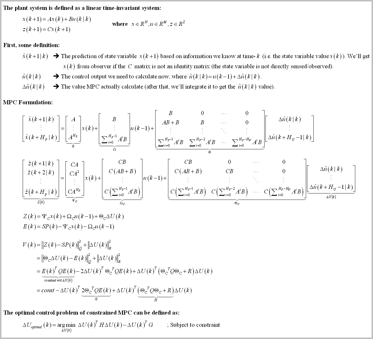
 As we can see here, the formulation of constrained MPC is exactly the same as
the unconstrained version. The difference is on the optimal control problem definition where the constrained version, well, has constraints.
As we can see here, the formulation of constrained MPC is exactly the same as
the unconstrained version. The difference is on the optimal control problem definition where the constrained version, well, has constraints.
As we can see here, the formulation of constrained MPC is exactly the same as
the unconstrained version. The difference is on the optimal control problem definition where the constrained version, well, has constraints.
 constraint (i.e.
  ), or the actuator slew rate constraint.
2.
), or the actuator slew rate constraint.
2.  constraint (i.e.
  ), or the actuator output constraint.
3.
), or the actuator output constraint.
3.  constraint (i.e.
  ), or the system output constraint.
**Remark**: To make the explanation simple and complete, in this implementation I implemented all constraints. But in the real implementation, you don't need to. For example, for you can implement the minimum constraint only (without the maximum constraint)
), or the system output constraint.
**Remark**: To make the explanation simple and complete, in this implementation I implemented all constraints. But in the real implementation, you don't need to. For example, for you can implement the minimum constraint only (without the maximum constraint)  . Or for example if you have 3 input, you can limit only the second input
  and set free the other. *Actually it is preferred (best practice) to implement hard-contraints as little as possible to ensure maximum feasible search space*.
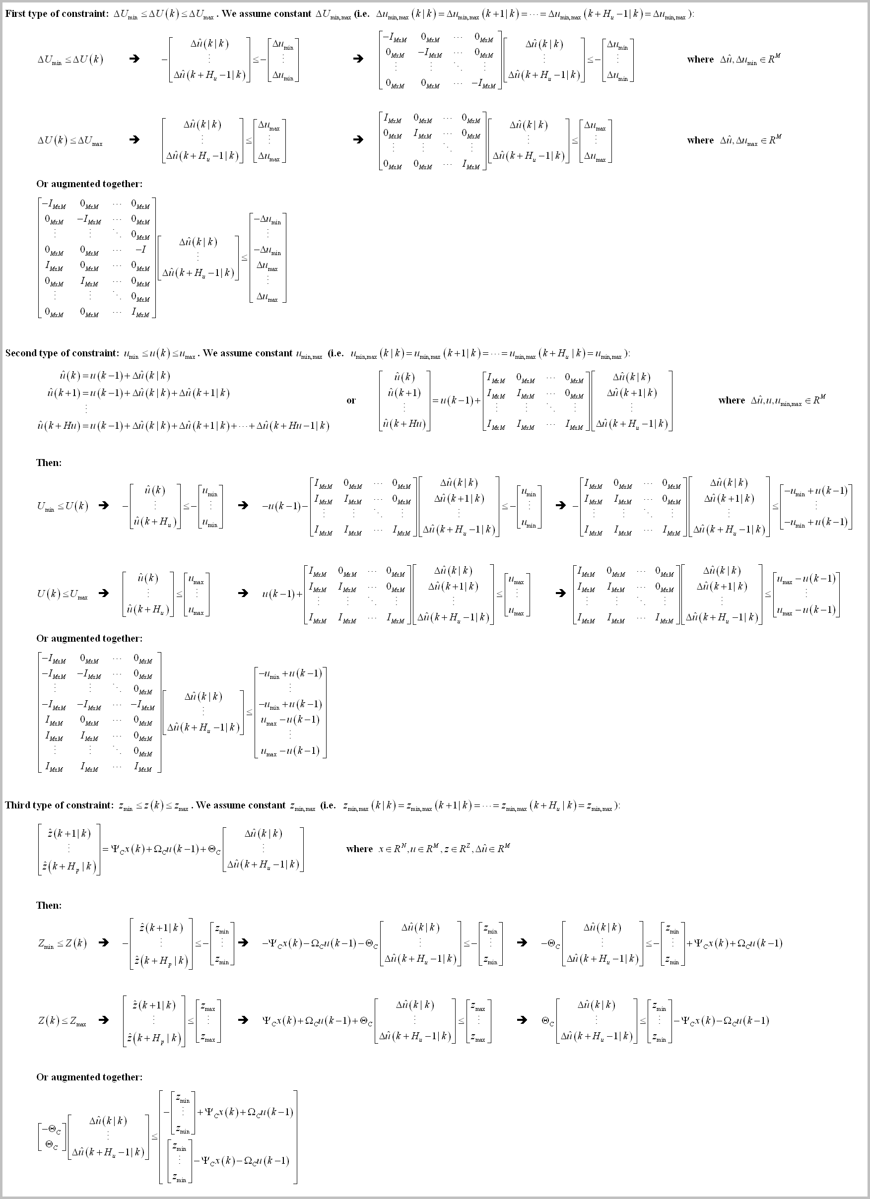
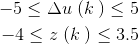
The constraints formulation can be described as:
and set free the other. *Actually it is preferred (best practice) to implement hard-contraints as little as possible to ensure maximum feasible search space*.
The constraints formulation can be described as:
 welp, I guess that's all XD
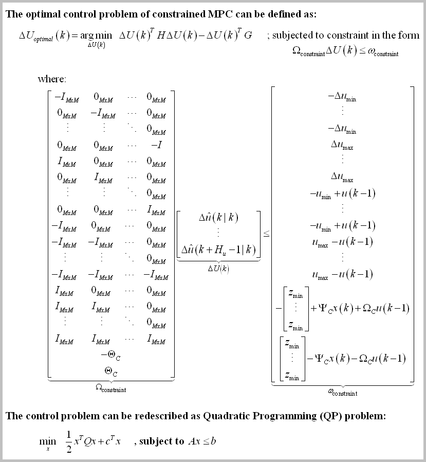 **Note**: From this point onward, sometimes I'll use `MPC` subscript to denote MPC variables and `QP` subscript to denote Quadratic Programming solver variables. But if the context is known (e.g. In the MPC subsection/Active Set subsection), I'll drop the subscript to shorten the explanation.
In the formulation above,
**Note**: From this point onward, sometimes I'll use `MPC` subscript to denote MPC variables and `QP` subscript to denote Quadratic Programming solver variables. But if the context is known (e.g. In the MPC subsection/Active Set subsection), I'll drop the subscript to shorten the explanation.
In the formulation above,  means when we call the QP solver from MPC subroutine, we need to scale the MPC variables accordingly
  .
# The Quadratic Programming Solver
In this implementation, I use (one of [several](https://en.wikipedia.org/wiki/Quadratic_programming#Solution_methods)) QP solver called [Active Set methods (ASM)](https://en.wikipedia.org/wiki/Active-set_method). The big idea of active set algorithm is searching the optimal
.
# The Quadratic Programming Solver
In this implementation, I use (one of [several](https://en.wikipedia.org/wiki/Quadratic_programming#Solution_methods)) QP solver called [Active Set methods (ASM)](https://en.wikipedia.org/wiki/Active-set_method). The big idea of active set algorithm is searching the optimal  value by solving the QP problem (with inequality constraints) as QP problem with equality constraints (EQP). More concretely, we search by iterating through EQP subproblem, and construct the EQP subproblem (more specifically the constraint matrix) from the set of QP constraints that is active at that iteration (hence the name).
In the wild, many recent reseach are using the more 'sexy' solver like [Interior Point methods (IPM)](https://en.wikipedia.org/wiki/Interior-point_method) because the IPM is faster for big QP problem. But in our case (i.e. MPC implementation for embedded system) we mainly deal with small (less than ten) state variables/actuator and small (less than twenty) prediction horizon (we're limited by the RAM size after all). In that case, the ASM will be faster than IPM. And by exploiting the MPC structure, we can reduce the computation time even further while increase the numerical stability (see [Active Set note: Solving the Linear Equation of KKT system](README.md#active-set-note-solving-the-linear-equation-of-kkt-system) subsection and [The MPC Implementation](README.md#the-second-implementation-optimized-active-set-with-schur-complement-of-kkt) subsection below).
On the [Wikipedia page](https://en.wikipedia.org/wiki/Active-set_method), the general structure of an active set algorithm is:
```
Find a feasible starting point
repeat until "optimal enough"
solve the equality problem defined by the active set (approximately)
compute the Lagrange multipliers of the active set
remove a subset of the constraints with negative Lagrange multipliers
search for infeasible constraints
end repeat
```
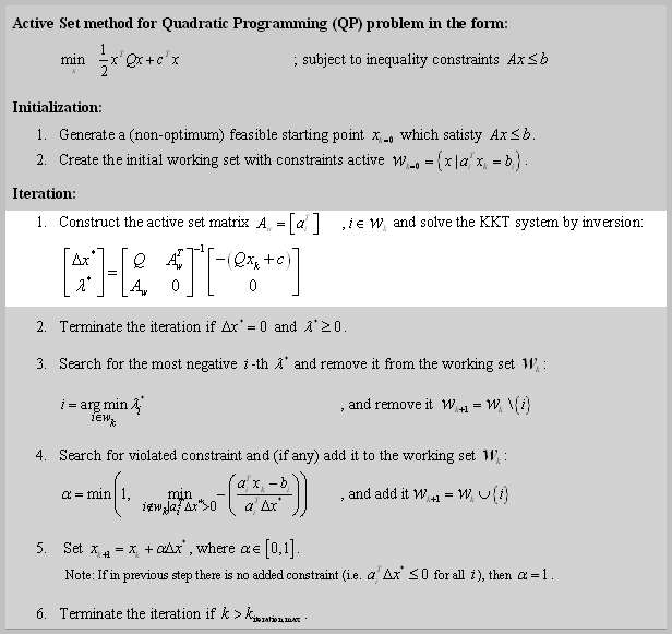
Using above structure, the active set algorithm used in this implementation can be described as:
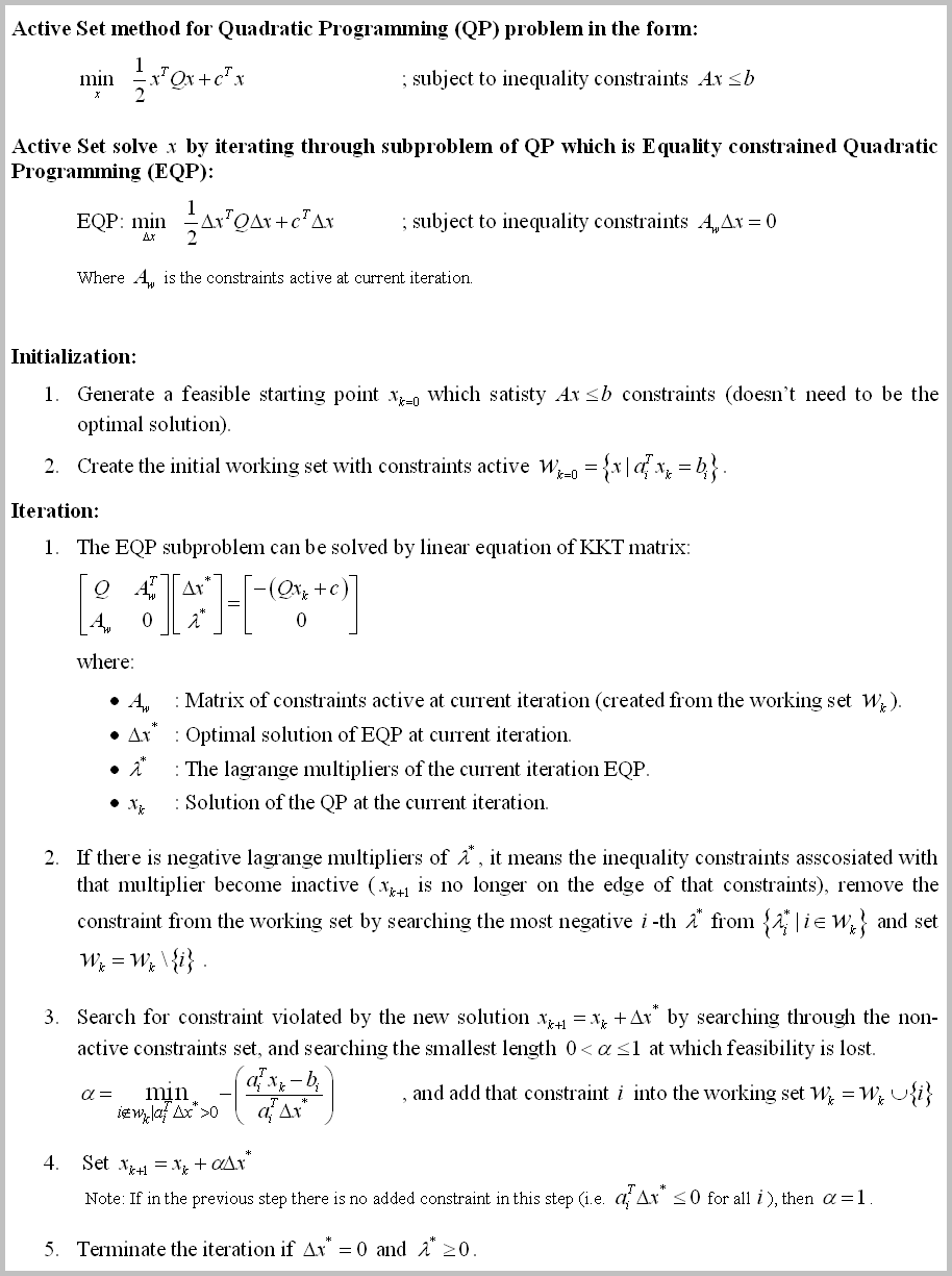
**Remark**: If the global optimum is inside the feasible region (i.e. the global optimum doesn't violate any constraints) and is not on the edge of any constraint, then it means there is no constraint active and the active set matrix
value by solving the QP problem (with inequality constraints) as QP problem with equality constraints (EQP). More concretely, we search by iterating through EQP subproblem, and construct the EQP subproblem (more specifically the constraint matrix) from the set of QP constraints that is active at that iteration (hence the name).
In the wild, many recent reseach are using the more 'sexy' solver like [Interior Point methods (IPM)](https://en.wikipedia.org/wiki/Interior-point_method) because the IPM is faster for big QP problem. But in our case (i.e. MPC implementation for embedded system) we mainly deal with small (less than ten) state variables/actuator and small (less than twenty) prediction horizon (we're limited by the RAM size after all). In that case, the ASM will be faster than IPM. And by exploiting the MPC structure, we can reduce the computation time even further while increase the numerical stability (see [Active Set note: Solving the Linear Equation of KKT system](README.md#active-set-note-solving-the-linear-equation-of-kkt-system) subsection and [The MPC Implementation](README.md#the-second-implementation-optimized-active-set-with-schur-complement-of-kkt) subsection below).
On the [Wikipedia page](https://en.wikipedia.org/wiki/Active-set_method), the general structure of an active set algorithm is:
```
Find a feasible starting point
repeat until "optimal enough"
solve the equality problem defined by the active set (approximately)
compute the Lagrange multipliers of the active set
remove a subset of the constraints with negative Lagrange multipliers
search for infeasible constraints
end repeat
```
Using above structure, the active set algorithm used in this implementation can be described as:

**Remark**: If the global optimum is inside the feasible region (i.e. the global optimum doesn't violate any constraints) and is not on the edge of any constraint, then it means there is no constraint active and the active set matrix  disappear. The KKT system equation simply becomes:
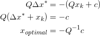
 , then the optimal control calculation becomes
  which exactly is the equation for [unconstrained MPC](https://github.com/pronenewbits/Arduino_Unconstrained_MPC_Library/blob/master/Formulation_of_Optimal_Control.png)! With this we can prove that the constrained MPC using active set solver is a generalization of unconstrained MPC (math is pretty nifty huh).
#### Active Set note: The Termination Condition
The termination condition on the last line of algorithm above
which exactly is the equation for [unconstrained MPC](https://github.com/pronenewbits/Arduino_Unconstrained_MPC_Library/blob/master/Formulation_of_Optimal_Control.png)! With this we can prove that the constrained MPC using active set solver is a generalization of unconstrained MPC (math is pretty nifty huh).
#### Active Set note: The Termination Condition
The termination condition on the last line of algorithm above  is called [Karush–Kuhn–Tucker conditions](https://en.wikipedia.org/wiki/Karush%E2%80%93Kuhn%E2%80%93Tucker_conditions). As the condition is applied on the solution of the KKT system on EQP subproblem (first line on iteration), then we can move the termination check just after we solve the KKT system.
#### Active Set note: Programming Implementation
The simplest way to implement the active set
is called [Karush–Kuhn–Tucker conditions](https://en.wikipedia.org/wiki/Karush%E2%80%93Kuhn%E2%80%93Tucker_conditions). As the condition is applied on the solution of the KKT system on EQP subproblem (first line on iteration), then we can move the termination check just after we solve the KKT system.
#### Active Set note: Programming Implementation
The simplest way to implement the active set  is by using an array of boolean, where the size of the array is as big as the number of constraints. That way, the operation of adding or removing the *i*-th constraint into/from (i.e. the
  and
and  operations) simply becomes the operation of setting the *i*-th value of the array as `true` or `false`, accordingly.
#### Active Set note: Generating the Feasible Starting Point
todo: calculate the starting point using linear programming. For now we set the starting point as zero (ok if the null space of x is inside the feasible search space, e.g. du_mpc,min < 0 and du_mpc,max > 0).
#### Active Set note: Solving the Linear Equation of KKT system
The most obvious way to solve the KKT system is by inverting the LHS matrix of the KKT equation (e.g. using Gauss-Jordan elimination):
operations) simply becomes the operation of setting the *i*-th value of the array as `true` or `false`, accordingly.
#### Active Set note: Generating the Feasible Starting Point
todo: calculate the starting point using linear programming. For now we set the starting point as zero (ok if the null space of x is inside the feasible search space, e.g. du_mpc,min < 0 and du_mpc,max > 0).
#### Active Set note: Solving the Linear Equation of KKT system
The most obvious way to solve the KKT system is by inverting the LHS matrix of the KKT equation (e.g. using Gauss-Jordan elimination):

 matrix as a symmetric positive definite matrix, and moreover, a constant matrix.
Both approach to solve the KKT system is implemented below (as [naive implementation](README.md#the-first-implementation-the-naive-implementation) and [Schur complement implementation](README.md#the-second-implementation-optimized-active-set-with-schur-complement-of-kkt)).
#### Active Set note: Additional Termination Condition
Unlike unconstrained MPC (where the solver is [basically a gain matrix](https://github.com/pronenewbits/Arduino_Unconstrained_MPC_Library#the-second-implementation-description-optimized-version-of-the-naive-implementation)), the constrained MPC solver use iteration to calculate the optimal control value (QP in worst case is NP-hard). It means in a real-time system, in worst case we need to terminate the iteration before the optimal control value can be calculated.
The nifty thing about ASM is that once we have optimal variable
matrix as a symmetric positive definite matrix, and moreover, a constant matrix.
Both approach to solve the KKT system is implemented below (as [naive implementation](README.md#the-first-implementation-the-naive-implementation) and [Schur complement implementation](README.md#the-second-implementation-optimized-active-set-with-schur-complement-of-kkt)).
#### Active Set note: Additional Termination Condition
Unlike unconstrained MPC (where the solver is [basically a gain matrix](https://github.com/pronenewbits/Arduino_Unconstrained_MPC_Library#the-second-implementation-description-optimized-version-of-the-naive-implementation)), the constrained MPC solver use iteration to calculate the optimal control value (QP in worst case is NP-hard). It means in a real-time system, in worst case we need to terminate the iteration before the optimal control value can be calculated.
The nifty thing about ASM is that once we have optimal variable  candidate that is inside feasible region, the next iteration of the variable
  will be both:
a) Also inside the feasible region; and
b) More optimal than the previous iteration.
Using that fact, we can easily add another termination condition
will be both:
a) Also inside the feasible region; and
b) More optimal than the previous iteration.
Using that fact, we can easily add another termination condition  beside KKT condition to make sure the MPC calculation still satisfy the real-time requirement. The other option is to use a real-time timer as the termination condition. We then can use the not-the-most-optimal-but-still-feasible solution as the controller output.
#### Active Set: Wrap it up
The Active Set pseudo code then can be redescribed as:
beside KKT condition to make sure the MPC calculation still satisfy the real-time requirement. The other option is to use a real-time timer as the termination condition. We then can use the not-the-most-optimal-but-still-feasible solution as the controller output.
#### Active Set: Wrap it up
The Active Set pseudo code then can be redescribed as:
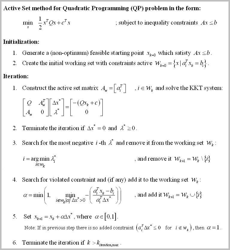
 while we use
  (just multiply the inequality with
  to change from one form to another).
# The MPC Implementation
The implementations of the MPC control calculation consist of two main implementations, each of the implementation is self contained in each folder and calculate the same control output (theoretically).
### The first implementation: The Naive Implementation
The Naive Implementation algorithm is just a direct implementation of the MPC derivation above. The MPC algorithm can be described as (the source code can be found in "[mpc_constrained_naive_engl](mpc_constrained_naive_engl)" folder, especially see "[mpc.cpp](mpc_constrained_naive_engl/mpc.cpp)" file):
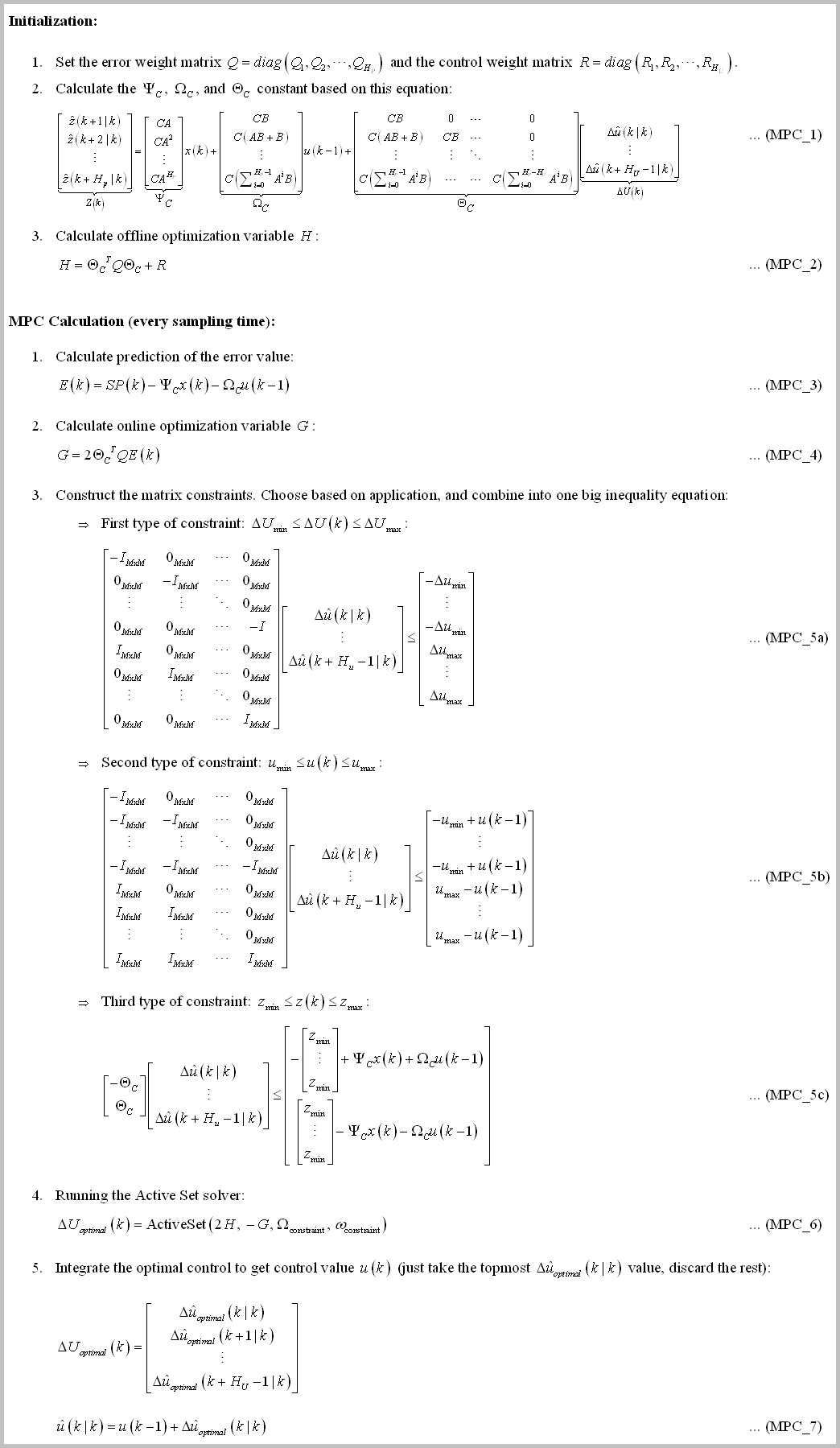
The active set subroutine is exactly [the same as explained above](README.md#active-set-wrap-it-up) where the KKT solution is calculated by matrix inversion (the code is also inside "[mpc.cpp](mpc_constrained_naive_engl/mpc.cpp#L240)" file):
to change from one form to another).
# The MPC Implementation
The implementations of the MPC control calculation consist of two main implementations, each of the implementation is self contained in each folder and calculate the same control output (theoretically).
### The first implementation: The Naive Implementation
The Naive Implementation algorithm is just a direct implementation of the MPC derivation above. The MPC algorithm can be described as (the source code can be found in "[mpc_constrained_naive_engl](mpc_constrained_naive_engl)" folder, especially see "[mpc.cpp](mpc_constrained_naive_engl/mpc.cpp)" file):

The active set subroutine is exactly [the same as explained above](README.md#active-set-wrap-it-up) where the KKT solution is calculated by matrix inversion (the code is also inside "[mpc.cpp](mpc_constrained_naive_engl/mpc.cpp#L240)" file):
 portion) is actually constant. We should move them into MPC initialization step.
3. If we limit the selection of the MPC `Q` and `R` weight matrices as diagonal and all its entry positive (in fact we've been doing it since [the unconstrained implementation](https://github.com/pronenewbits/Arduino_Unconstrained_MPC_Library#the-background)), then
portion) is actually constant. We should move them into MPC initialization step.
3. If we limit the selection of the MPC `Q` and `R` weight matrices as diagonal and all its entry positive (in fact we've been doing it since [the unconstrained implementation](https://github.com/pronenewbits/Arduino_Unconstrained_MPC_Library#the-background)), then  is also a symmetric positive definite matrix (here I denote `Q` and `R` weight matrices with `MPC` subscript to differentiate them with `Q` matrix of QP solver).
Based on the last point, we can speed up the solution calculation of the KKT system:
is also a symmetric positive definite matrix (here I denote `Q` and `R` weight matrices with `MPC` subscript to differentiate them with `Q` matrix of QP solver).
Based on the last point, we can speed up the solution calculation of the KKT system:

as the pivot. Then the KKT system will becomes:

 , and the solution of KKT system then can be calculated as:

 matrix is constant, so also its inverse.
2. As the is positive definite, so is the matrix
matrix is constant, so also its inverse.
2. As the is positive definite, so is the matrix  . It means we can use [Cholesky decomposition to solve the first equation](https://en.wikipedia.org/wiki/Cholesky_decomposition#Applications) instead of calculating the inversion of it. Whenever applicable, the Cholesky decomposition is faster and more stable numerically than Gaussian elimination.
3. In many cases, the active set matrix dimension is smaller than dimension, so the matrix will be smaller than and obviously smaller than , making the computation even more faster, relative to the naive inversion.
4. For the MPC calculation, the KKT matrix is the biggest matrix constructed. By avoid constructing it, we can reduce the memory used by the MPC.
\* As [stated on the unconstrained version](https://github.com/pronenewbits/Arduino_Unconstrained_MPC_Library#the-third-implementation-description-the-numerically-robust-version), if we don't take care of it, the
. It means we can use [Cholesky decomposition to solve the first equation](https://en.wikipedia.org/wiki/Cholesky_decomposition#Applications) instead of calculating the inversion of it. Whenever applicable, the Cholesky decomposition is faster and more stable numerically than Gaussian elimination.
3. In many cases, the active set matrix dimension is smaller than dimension, so the matrix will be smaller than and obviously smaller than , making the computation even more faster, relative to the naive inversion.
4. For the MPC calculation, the KKT matrix is the biggest matrix constructed. By avoid constructing it, we can reduce the memory used by the MPC.
\* As [stated on the unconstrained version](https://github.com/pronenewbits/Arduino_Unconstrained_MPC_Library#the-third-implementation-description-the-numerically-robust-version), if we don't take care of it, the  (although a constant) is often ill conditioned. So care must be taken to make sure the will behave as good as possible.
The MPC algorithm then can be described as (the source code can be found in "[mpc_constrained_schur_engl](mpc_constrained_schur_engl)" folder, especially see "[mpc.cpp](mpc_constrained_schur_engl/mpc.cpp)" file):
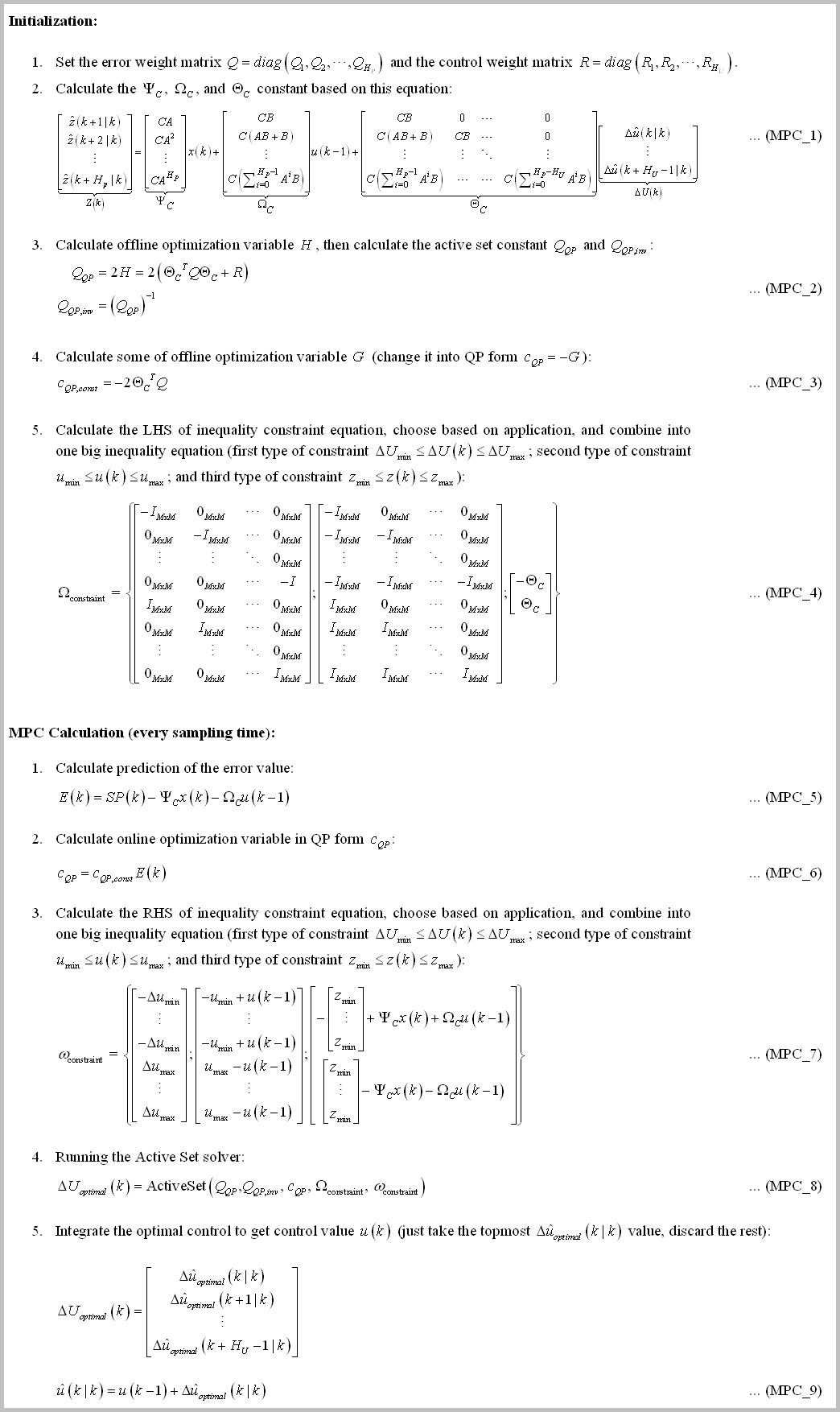
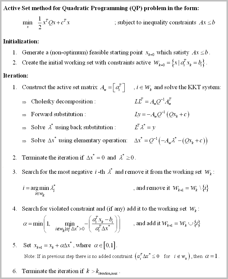
Where the active set subroutine can be described as (the code is also inside "[mpc.cpp](mpc_constrained_schur_engl/mpc.cpp#L256)" file):
(although a constant) is often ill conditioned. So care must be taken to make sure the will behave as good as possible.
The MPC algorithm then can be described as (the source code can be found in "[mpc_constrained_schur_engl](mpc_constrained_schur_engl)" folder, especially see "[mpc.cpp](mpc_constrained_schur_engl/mpc.cpp)" file):

Where the active set subroutine can be described as (the code is also inside "[mpc.cpp](mpc_constrained_schur_engl/mpc.cpp#L256)" file):
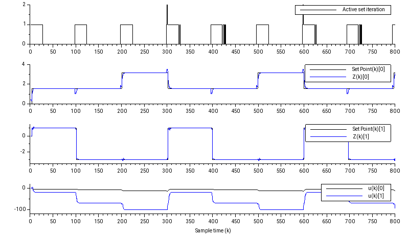
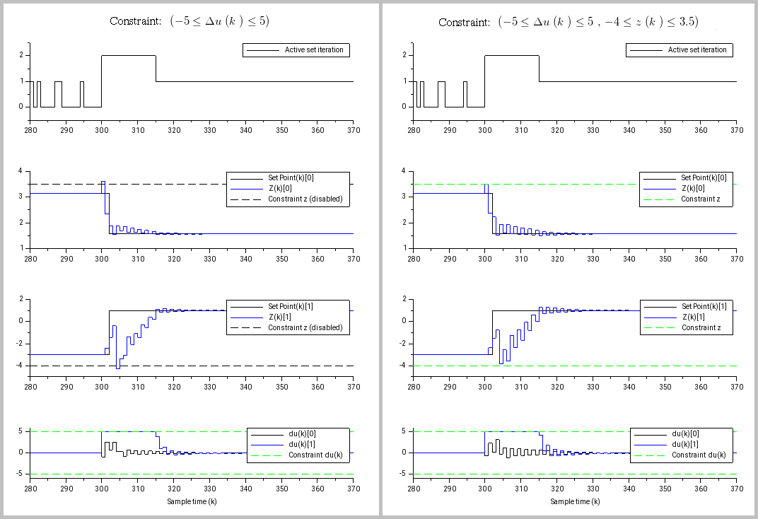
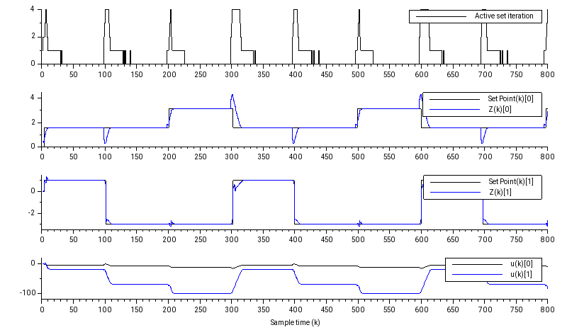
 : Maximum 4 active-set iterations. Take attention that the signals become slower to change.
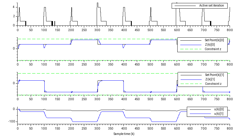
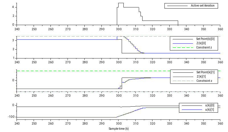
 : Maximum 5 active-set iterations. Take attention that beside the signals become slower to change, the output at ~300th sampling time don't overshoot anymore.
|Constraints Configuration|Maximum Active Set iteration|Naive Implementation|Implementation using Schur Complement|Schur Complement without Bounds Checking|
|:---:|:---:|:----:|:---:|:---:|
|No-constraint|2|169 us|35 us|11 us|
||4|556 us|170 us|67 us|
| |5|886 us
(117.2 us/iteration)|327 us
(65.4 us/iteration)|127 us
(25.4 us/iteration)|
(Nice)
matrix doesn't need to be positive definite), Conjugate gradient method, etc. Refer to mathematical optimization textbooks to read more on this topic.
The interesting thing happens when we disabled the matrix bounds checking in `konfig.h` (if you customize/change the plant system, you need to harden the system before disable it), we can get further increase throughput 2 to 4 times compared with bounds checking enabled, where the best result is **127 us** for a fully functioning constrained MPC. That means this MPC library is capable to tackle a reasonably complex very fast system at several hundred (or even thousand) Hz sampling rate (and in a $20 hardware form!).
Using static analyzer, the biggest matrix constructed is matrix where the worst-case size is `(2xHuxM) + (2xHpxZ)` when we enable constraints. The matrix maximum size will be `(2x4x2)+(2x3x2) = 28`. This is the `MATRIX_MAXIMUM_SIZE` value we used in this benchmark.
Note that when we use the naive version, the worst case matrix size is actually the dimension of which is `(HpxZ) + (2xHuxM) + (2xHpxZ)` or 36 (we don't use it here because of stack overflow).
### More Interesting Benchmark
Sometimes I just want to see how far I can push this system to the extreme. Using the same model (Jet Transport Aircraft), the lowest `Hp` & `Hu` values that still capable to tracking the set point are `Hp=3` and `Hu=1` (with degraded transient response). The biggest matrix is with constraints at the size `(2*Hu*M)+(2*Hp*Z) x (Hu*M) = (2*1*2)+(2*3*2)x(1*2) = 16x2 matrix`.
The benchmark data variable `_maxu64compuTime`, in microseconds are (lower is better):
|Constraints Configuration|Maximum Active Set iteration|Implementation using Schur Complement|Schur Complement without Bounds Checking|
|:---:|:---:|:----:|:---:|
|No-constraint|1|11 us|4 us|
||2|26 us|13 us|
||2|52 us|28 us|
(Noice) With this we're entering the tens to (almost) hundred kHz application (\*⌄\*)
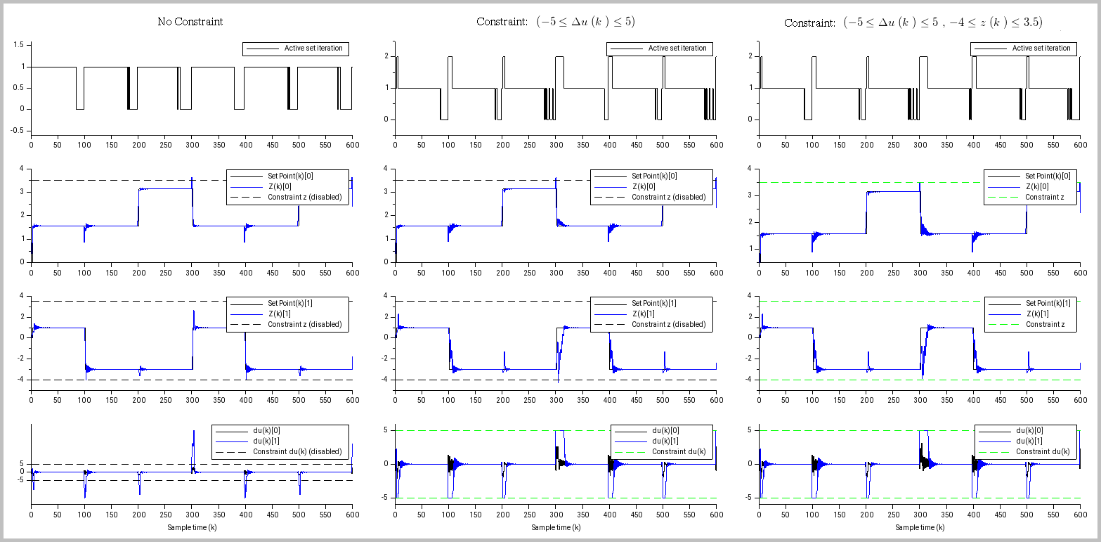
and constraints (the MPC still able to control the system while still comply with the constraints):