{
"cells": [
{
"cell_type": "markdown",
"metadata": {},
"source": [
"# Data Analysis using Jupyter Notebooks Part 2\n",
"\n",
"Benjamin J. Morgan\n",
"\n",
"# Tutorial 1\n",
"\n",
"\n",
"In the CH10009 “Data Analysis using Jupyter Notebooks” you were introduced to simple programmatic data analysis and plotting using the Python programming language and Jupyter Notebooks. This practical builds on that previous activity. By working through these notebooks, you will \n",
"1. Revisit the key ideas from the Part 1 practical, giving you more experience and practice writing your own code.\n",
"2. Learn how to write your own functions, which can then be used to organise your code, and to perform more sophistocated data analyses.\n",
"\n",
"## Assessment\n",
"\n",
"The assessment of this practical has two components:\n",
"\n",
"1. After completing **Exercise 3**, save your final notebook (using **File > Save and Checkpoint** in the Jupyter menu), and upload this .ipynb file to Moodle. Please make sure that you have run your notebook from a fresh start, and that it works as expected, before saving and submitting (**Kernel > Restart and Run All** from the Jupyter menu).\n",
"2. A Moodle quiz.\n",
"\n",
"\n",
"## Review of Part 1\n",
"\n",
"The CH10009 Part 1 practical covered the following concepts:\n",
"- Introduction to Jupyter notebooks\n",
" - Opening Jupyter notebooks\n",
" - Running code\n",
"- Code versus Markdown cells\n",
"- Importing modules\n",
"- Mathematical functions\n",
"- Variables\n",
"- Numbers, Strings, and Lists\n",
"- `numpy` and arrays\n",
"- Plotting data with `matplotlib`\n",
" - line styles\n",
" - formatting points\n",
" - labelling axes and adding titles\n",
" - saving to a PDF\n",
"- Introduction to data analysis and statistics, using `numpy`:\n",
" - Some useful `numpy` functions: `min()`, `max()`, `sum()`, `mean()`, `std()`\n",
" - linear regression, using `scipy.stats.linregress`\n",
" \n",
"In this practical you will quickly review these concepts, before building on these to develop your programming and data analysis skills. This review of the Part 1 material will be fairly compact, so if there are any parts you are unsure about, remember that you can always review your Part 1 Tutorial notebooks. These will either still be on your `H:` drive, or you can download them from the [CH10009 Moodle page](https://moodle.bath.ac.uk/course/view.php?id=538). You can also insert new code cells to run any bits of code you like, to check that you understand how the examples work. Code cells can be inserted into any notebook using **Insert > Insert Cell Above** or **Insert > Insert Cell Below** from the Jupyter menu. "
]
},
{
"cell_type": "markdown",
"metadata": {},
"source": [
"## Using Jupyter notebooks\n",
"\n",
"A Jupyter notebook consists of a series of **cells** that contain text. These cells are arranged vertically, top-to-bottom in the document. Any cell can be edited by clicking on it. A cell in **edit mode** is indicated by a green border. \n",
" \n",
"A cell with a blue border is in **command mode**. \n",
"
\n",
"A cell with a blue border is in **command mode**. \n",
" \n",
"In command mode you are not able to type into a cell, but you can still edit the notebook (reordering cells, executing code, etc.) Commands for editing notebooks can be accessed from the manu at the top of the screen, and commonly used commands have keyboard shortcuts, which will be highlighted in examples using green text. The full list of keyboard shortcuts can be found through **Help > Keyboard Shortcuts** in the menu.\n",
"\n",
"To edit a cell in command mode, press enter or double click on the cell."
]
},
{
"cell_type": "markdown",
"metadata": {},
"source": [
"## Running Code \n",
"\n",
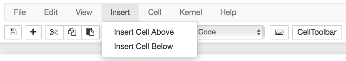
"The default cell type in a Jupyter notebook is a **code** cell. If you open a new notebook it will have one, empty, code cell. And you can always create more cells by clicking in the menu on **Insert > Insert Cell Above** (a) or **Insert > Insert Cell Below** (b). \n",
"
\n",
"In command mode you are not able to type into a cell, but you can still edit the notebook (reordering cells, executing code, etc.) Commands for editing notebooks can be accessed from the manu at the top of the screen, and commonly used commands have keyboard shortcuts, which will be highlighted in examples using green text. The full list of keyboard shortcuts can be found through **Help > Keyboard Shortcuts** in the menu.\n",
"\n",
"To edit a cell in command mode, press enter or double click on the cell."
]
},
{
"cell_type": "markdown",
"metadata": {},
"source": [
"## Running Code \n",
"\n",
"The default cell type in a Jupyter notebook is a **code** cell. If you open a new notebook it will have one, empty, code cell. And you can always create more cells by clicking in the menu on **Insert > Insert Cell Above** (a) or **Insert > Insert Cell Below** (b). \n",
" \n",
"Any code typed into a code cell can be run (or \"**executed**\") by pressing `Shift-Enter` or pressing the
\n",
"Any code typed into a code cell can be run (or \"**executed**\") by pressing `Shift-Enter` or pressing the  button in the notebook toolbar.\n",
"\n",
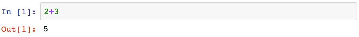
"This practical consists of an interactive tutorial (this notebook), followed by a a series of exercises. Some code cells in the tutorial will already have code in them, which you can **run** by selecting and pressing `Shift-Enter` or clicking the toolbar button:"
]
},
{
"cell_type": "code",
"execution_count": 2,
"metadata": {},
"outputs": [
{
"data": {
"text/plain": [
"5"
]
},
"execution_count": 2,
"metadata": {},
"output_type": "execute_result"
}
],
"source": [
"# run this cell\n",
"2 + 3"
]
},
{
"cell_type": "markdown",
"metadata": {},
"source": [
"You should now have Out[ ]: with the result of running this code printed next to it:\n",
"
button in the notebook toolbar.\n",
"\n",
"This practical consists of an interactive tutorial (this notebook), followed by a a series of exercises. Some code cells in the tutorial will already have code in them, which you can **run** by selecting and pressing `Shift-Enter` or clicking the toolbar button:"
]
},
{
"cell_type": "code",
"execution_count": 2,
"metadata": {},
"outputs": [
{
"data": {
"text/plain": [
"5"
]
},
"execution_count": 2,
"metadata": {},
"output_type": "execute_result"
}
],
"source": [
"# run this cell\n",
"2 + 3"
]
},
{
"cell_type": "markdown",
"metadata": {},
"source": [
"You should now have Out[ ]: with the result of running this code printed next to it:\n",
" \n",
"and the focus has automatically moved to the next cell. You can always re-select a cell to run it again."
]
},
{
"cell_type": "markdown",
"metadata": {},
"source": [
"You will see that after running a cell a number appears inside the square brackets next to the input code, and next to the output result, e.g. In [1]: and Out[1]:.\n",
"\n",
"If the square brackets next to a cell contain an asterisk, e.g. In [\\*]:, the code in this cell is either running, or is queued to run after another cell. \n",
"You can interrupt a running notebook using the **interrupt kernel** button
\n",
"and the focus has automatically moved to the next cell. You can always re-select a cell to run it again."
]
},
{
"cell_type": "markdown",
"metadata": {},
"source": [
"You will see that after running a cell a number appears inside the square brackets next to the input code, and next to the output result, e.g. In [1]: and Out[1]:.\n",
"\n",
"If the square brackets next to a cell contain an asterisk, e.g. In [\\*]:, the code in this cell is either running, or is queued to run after another cell. \n",
"You can interrupt a running notebook using the **interrupt kernel** button  in the toolbar."
]
},
{
"cell_type": "markdown",
"metadata": {},
"source": [
"## Rearranging Cells\n",
"\n",
"Because the content in a Jupyter notebook is arranged as a series of cells, it is easy to organise and reorganise your code and other content. \n",
"You can move cells up or down in the notebook by clicking the **move selected cells up** or **move selected cells down** buttons
in the toolbar."
]
},
{
"cell_type": "markdown",
"metadata": {},
"source": [
"## Rearranging Cells\n",
"\n",
"Because the content in a Jupyter notebook is arranged as a series of cells, it is easy to organise and reorganise your code and other content. \n",
"You can move cells up or down in the notebook by clicking the **move selected cells up** or **move selected cells down** buttons  in the toolbar.\n",
"\n",
"The ability to run cells in a notebook in any order makes working with notebooks very flexible, but can make it hard to keep track of what order you have run your cells. If your code is not working as you expect, this might be because the notebook cells have been run out of order. In this case, you can “reboot” the notebook, and run all the cells in their current order, by selecting **Kernel > Restart & Run All** from the Notebook menu."
]
},
{
"cell_type": "markdown",
"metadata": {},
"source": [
"## Saving Notebooks\n",
"\n",
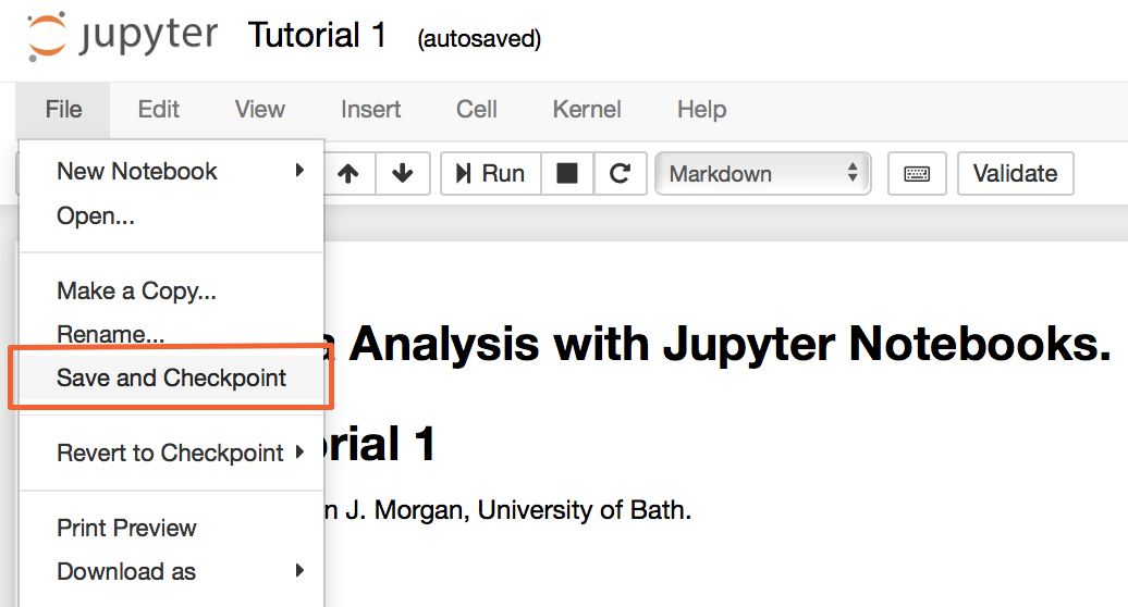
"To save your notebook, you can select **File > Save and Checkpoint** from the Jupyter menu, or use the keyboard shortcut **⌘+S** (on macOS) or **ctrl+S** (on Windows & Linux). Jupyter notebooks are saved as **.ipynb** files.\n",
"\n",
"
in the toolbar.\n",
"\n",
"The ability to run cells in a notebook in any order makes working with notebooks very flexible, but can make it hard to keep track of what order you have run your cells. If your code is not working as you expect, this might be because the notebook cells have been run out of order. In this case, you can “reboot” the notebook, and run all the cells in their current order, by selecting **Kernel > Restart & Run All** from the Notebook menu."
]
},
{
"cell_type": "markdown",
"metadata": {},
"source": [
"## Saving Notebooks\n",
"\n",
"To save your notebook, you can select **File > Save and Checkpoint** from the Jupyter menu, or use the keyboard shortcut **⌘+S** (on macOS) or **ctrl+S** (on Windows & Linux). Jupyter notebooks are saved as **.ipynb** files.\n",
"\n",
" \n",
"\n",
"You can make a copy of a notebook (for example, to save an old version while you work on a new idea, or to duplicate a notebook to a different directory) you can either select **File > Make a Copy**, which duplicates the current notebook in the same directory; or you can select **File > Download as > Notebook (.ipynb)**, to download a copy into your **Downloads**."
]
},
{
"cell_type": "markdown",
"metadata": {},
"source": [
"## Comments\n",
"\n",
"To help explain what a particular code does, or to explain *why* a piece of code is being used, you can include **comments**.\n",
"\n",
"```python\n",
"# this is comment\n",
"```\n",
"\n",
"Any text that appears after a # symbol is part of the comment, and is ignored when the code is run. \n",
"\n"
]
},
{
"cell_type": "markdown",
"metadata": {},
"source": [
"## Markdown Cells\n",
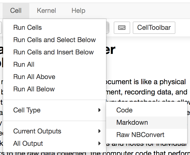
"Jupyter notebooks offer a second, more flexible, way to describe what your code is doing: **Markdown cells**. A code cell can be converted to a Markdown cell by selecting Cell > Cell Type > Markdown from the menu. \n",
"
\n",
"\n",
"You can make a copy of a notebook (for example, to save an old version while you work on a new idea, or to duplicate a notebook to a different directory) you can either select **File > Make a Copy**, which duplicates the current notebook in the same directory; or you can select **File > Download as > Notebook (.ipynb)**, to download a copy into your **Downloads**."
]
},
{
"cell_type": "markdown",
"metadata": {},
"source": [
"## Comments\n",
"\n",
"To help explain what a particular code does, or to explain *why* a piece of code is being used, you can include **comments**.\n",
"\n",
"```python\n",
"# this is comment\n",
"```\n",
"\n",
"Any text that appears after a # symbol is part of the comment, and is ignored when the code is run. \n",
"\n"
]
},
{
"cell_type": "markdown",
"metadata": {},
"source": [
"## Markdown Cells\n",
"Jupyter notebooks offer a second, more flexible, way to describe what your code is doing: **Markdown cells**. A code cell can be converted to a Markdown cell by selecting Cell > Cell Type > Markdown from the menu. \n",
" \n",
"A Markdown cell can be used to type plain text, which is displayed when the cell is run. Markdown cells are useful for documenting a notebook, particularly when you want to write something more detailed than a short comment. Markdown cells can also contain basic text formatting, links, images, and equations (more information is [here](http://jupyter-notebook.readthedocs.io/en/latest/examples/Notebook/Working%20With%20Markdown%20Cells.html))."
]
}
],
"metadata": {
"kernelspec": {
"display_name": "Python 3",
"language": "python",
"name": "python3"
},
"language_info": {
"codemirror_mode": {
"name": "ipython",
"version": 3
},
"file_extension": ".py",
"mimetype": "text/x-python",
"name": "python",
"nbconvert_exporter": "python",
"pygments_lexer": "ipython3",
"version": "3.6.1"
}
},
"nbformat": 4,
"nbformat_minor": 2
}
\n",
"A Markdown cell can be used to type plain text, which is displayed when the cell is run. Markdown cells are useful for documenting a notebook, particularly when you want to write something more detailed than a short comment. Markdown cells can also contain basic text formatting, links, images, and equations (more information is [here](http://jupyter-notebook.readthedocs.io/en/latest/examples/Notebook/Working%20With%20Markdown%20Cells.html))."
]
}
],
"metadata": {
"kernelspec": {
"display_name": "Python 3",
"language": "python",
"name": "python3"
},
"language_info": {
"codemirror_mode": {
"name": "ipython",
"version": 3
},
"file_extension": ".py",
"mimetype": "text/x-python",
"name": "python",
"nbconvert_exporter": "python",
"pygments_lexer": "ipython3",
"version": "3.6.1"
}
},
"nbformat": 4,
"nbformat_minor": 2
}