# giscoR
[](https://ropengov.org/)
[](https://CRAN.R-project.org/package=giscoR)
[](https://cran.r-project.org/web/checks/check_results_giscoR.html)
[](https://CRAN.R-project.org/package=giscoR)
[](https://ropengov.r-universe.dev/giscoR)
[](https://github.com/rOpenGov/giscoR/actions/workflows/check-full.yaml)
[](https://app.codecov.io/gh/ropengov/giscoR)
[](https://coveralls.io/github/rOpenGov/giscoR)
[](https://www.codefactor.io/repository/github/ropengov/giscor)
[](https://doi.org/10.32614/CRAN.package.giscoR)
[](https://www.repostatus.org/#active)
[**giscoR**](https://ropengov.github.io/giscoR/) is an **R** package
that provides a simple interface to the Eurostat [GISCO geodata
distribution](https://ec.europa.eu/eurostat/web/gisco). It lets you
download and work with global and European geospatial datasets directly
in **R**, including country boundaries, NUTS regions, administrative
units such as Local Administrative Units (LAU), statistical units,
transport networks and basic service locations.
## Key features
- Retrieve GISCO datasets for country boundaries, NUTS regions,
administrative units, statistical units, transport networks and basic
service locations.
- For compatible administrative and statistical datasets, select among
resolutions `60M`, `20M`, `10M`, `03M` and `01M`. Choose coordinate
reference systems **EPSG:4326**, **EPSG:3035** and **EPSG:3857**.
- Use each grid, transport or basic service dataset in its documented
format and coordinate reference system.
- Return **sf** objects for spatial analysis.
- Cache downloaded files for faster repeated access.
### Population grids
`gisco_get_grid()` downloads polygon or cell-center point GeoPackages in
**EPSG:3035** at resolutions from 1 km to 100 km. Population columns use
names such as `TOT_P_2021`. Divide these values by `resolution^2`, not
by `resolution`, to calculate people per square kilometer. Population
variables have year- and country-specific licensing conditions. Consult
the official [grid
documentation](https://ec.europa.eu/eurostat/web/gisco/geodata/grids)
before publication or redistribution.
## Installation
Install **giscoR** from
[**CRAN**](https://CRAN.R-project.org/package=giscoR):
``` r
install.packages("giscoR")
```
Check the documentation for the development version at
.
You can install the development version of **giscoR** with:
``` r
# install.packages("pak")
pak::pak("rOpenGov/giscoR")
```
Alternatively, you can install **giscoR** via
[**r-universe**](https://ropengov.r-universe.dev/giscoR):
``` r
install.packages(
"giscoR",
repos = c("https://ropengov.r-universe.dev", "https://cloud.r-project.org")
)
```
## Quick example
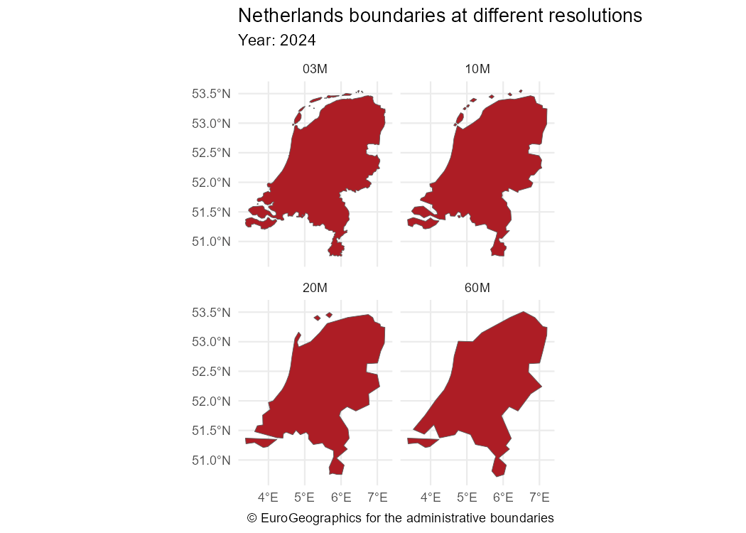
This example compares country boundaries at different resolutions:
``` r
library(giscoR)
library(sf)
library(dplyr)
# Download Netherlands boundaries at different resolutions.
nl_all <- lapply(c("60", "20", "10", "03"), function(r) {
gisco_get_countries(country = "Netherlands", year = 2024, resolution = r) |>
mutate(res = paste0(r, "M"))
}) |>
bind_rows()
glimpse(nl_all)
#> Rows: 4
#> Columns: 15
#> $ CNTR_ID "NL", "NL", "NL", "NL"
#> $ COUNTRY_URI "NLD", NA, "NLD", "NLD"
#> $ CNTR_NAME "Netherlands", "Nederland", "Netherlands", "Netherlands"
#> $ NAME_ENGL "Netherlands", "Netherlands", "Netherlands", "Netherlands"
#> $ NAME_FREN "Pays-Bas", "Pays-Bas", "Pays-Bas", "Pays-Bas"
#> $ ISO3_CODE "NLD", "NLD", "NLD", "NLD"
#> $ SVRG_UN "UN Member State", "UN Member State", "UN Member State", "…
#> $ CAPT "Amsterdam", "Amsterdam", "Amsterdam", "Amsterdam"
#> $ STAT_CODE "OA", NA, "OA", "OA"
#> $ EU_STAT "T", "T", "T", "T"
#> $ EFTA_STAT "F", "F", "F", "F"
#> $ CC_STAT "F", "F", "F", "F"
#> $ NAME_GERM "Niederlande", "Niederlande", "Niederlande", "Niederlande"
#> $ res "60M", "20M", "10M", "03M"
#> $ geometry MULTIPOLYGON (((7.208935 53..., MULTIPOLYGON (((7.202794 5…
# Plot with ggplot2.
library(ggplot2)
ggplot(nl_all) +
geom_sf(fill = "#AD1D25") +
facet_wrap(~res) +
labs(
title = "Netherlands boundaries at different resolutions",
subtitle = "Year: 2024",
caption = gisco_attributions()
) +
theme_minimal()
```
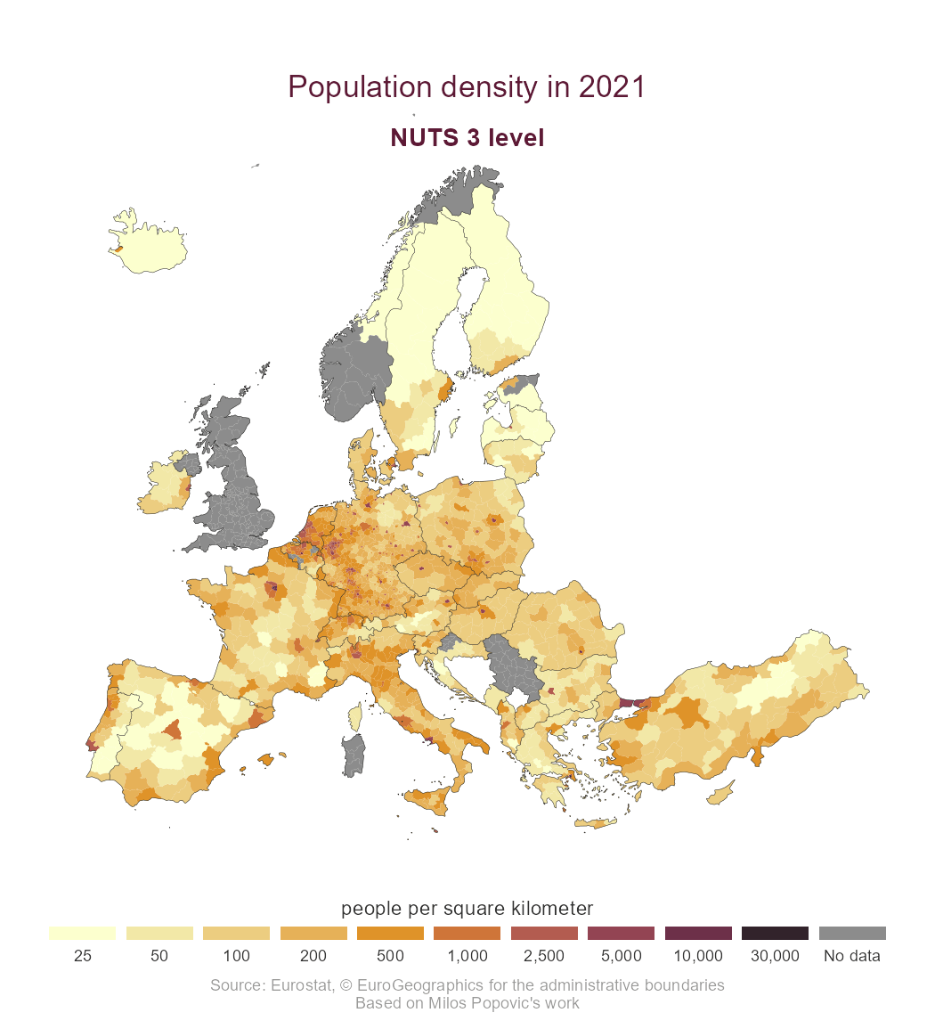
## Advanced example: thematic maps
This example shows a thematic map created with the **ggplot2** package.
The statistical data are retrieved with the **eurostat** package,
following the work of [Milos Popovic](https://milospopovic.net/).
Start by downloading the corresponding geospatial data:
``` r
library(giscoR)
library(dplyr)
library(eurostat)
library(ggplot2)
# Retrieve sf objects.
nuts3 <- gisco_get_nuts(
year = 2021,
epsg = 3035,
resolution = 10,
nuts_level = 3
)
# Get country boundaries at NUTS 0 level.
country_lines <- gisco_get_nuts(
year = 2021,
epsg = 3035,
resolution = 10,
spatialtype = "BN",
nuts_level = 0
)
```
Next, download the statistical data from Eurostat.
``` r
# Retrieve Eurostat data.
popdens <- get_eurostat("demo_r_d3dens") |>
filter(TIME_PERIOD == "2021-01-01")
```
Finally, merge and transform the datasets to create the plot.
``` r
# Merge data.
nuts3_sf <- nuts3 |>
left_join(popdens, by = "geo")
# Create breaks and labels.
br <- c(0, 25, 50, 100, 200, 500, 1000, 2500, 5000, 10000, 30000)
labs <- prettyNum(br[-1], big.mark = ",")
# Label missing values in the plot.
labeller_plot <- function(x) {
ifelse(is.na(x), "No data", x)
}
nuts3_sf <- nuts3_sf |>
# Cut with labels.
mutate(values_cut = cut(values, br, labels = labs))
# Create palette.
pal <- hcl.colors(length(labs), "Lajolla")
# Create plot.
ggplot(nuts3_sf) +
geom_sf(aes(fill = values_cut), linewidth = 0, color = NA, alpha = 0.9) +
geom_sf(data = country_lines, col = "black", linewidth = 0.1) +
# Center on Europe with EPSG 3035.
coord_sf(
xlim = c(2377294, 7453440),
ylim = c(1313597, 5628510)
) +
# Configure legends.
scale_fill_manual(
values = pal,
# Label missing values.
labels = labeller_plot,
drop = FALSE,
guide = guide_legend(direction = "horizontal", nrow = 1)
) +
theme_void() +
# Configure the theme.
theme(
plot.title = element_text(
color = rev(pal)[2],
size = rel(1.5),
hjust = 0.5,
vjust = -6
),
plot.subtitle = element_text(
color = rev(pal)[2],
size = rel(1.25),
hjust = 0.5,
vjust = -10,
face = "bold"
),
plot.caption = element_text(color = "grey60", hjust = 0.5, vjust = 0),
legend.text = element_text(color = "grey20", hjust = 0.5),
legend.title = element_text(color = "grey20", hjust = 0.5),
legend.position = "bottom",
legend.title.position = "top",
legend.text.position = "bottom",
legend.key.height = unit(0.5, "line"),
legend.key.width = unit(2.5, "line")
) +
# Add labels.
labs(
title = "Population density in 2021",
subtitle = "NUTS 3 level",
fill = "people per square kilometer",
caption = paste0(
"Source: Eurostat, ",
gisco_attributions(),
"\nBased on Milos Popovic's work"
)
)
```
## Caching
Large datasets, such as LAU or high-resolution files, can exceed 50 MB.
Set a cache directory with:
``` r
gisco_set_cache_dir("./path/to/location")
```
Files are stored in the local cache for faster repeated access.
## Contributing
See the [**GitHub** repository](https://github.com/rOpenGov/giscoR/) for
source code.
Contributions are welcome.
- Use the [issue tracker](https://github.com/rOpenGov/giscoR/issues) for
feedback and bug reports.
- Send [pull requests](https://github.com/rOpenGov/giscoR/).
- Star [**giscoR** on **GitHub**](https://github.com/rOpenGov/giscoR).
## Citation
To cite ‘giscoR’ in publications use:
Hernangómez D (2026). *giscoR: Download Eurostat GISCO Spatial Data*.
doi:10.32614/CRAN.package.giscoR
.
.
A **BibTeX** entry for **LaTeX** users is:
@Manual{R-giscoR,
title = {{giscoR}: Download Eurostat GISCO Spatial Data},
doi = {10.32614/CRAN.package.giscoR},
author = {Diego Hernangómez},
year = {2026},
version = {1.3.0},
url = {https://ropengov.github.io/giscoR/},
abstract = {Tools to download global and European spatial data from the Eurostat GISCO (Geographic Information System of the Commission) data distribution . The package provides helpers for country boundaries, Nomenclature of Territorial Units for Statistics (NUTS) regions, administrative units, statistical units, transport networks, basic service locations and other GISCO datasets. This package is neither affiliated with nor endorsed by Eurostat.},
}
## General copyright
[Eurostat’s general copyright notice and license
policy](https://ec.europa.eu/eurostat/web/main/help/copyright-notice)
applies. Some datasets have additional download and usage provisions.
The download and use of these data are subject to acceptance of those
provisions. See the [administrative
units](https://ec.europa.eu/eurostat/web/gisco/geodata/administrative-units)
and [statistical
units](https://ec.europa.eu/eurostat/web/gisco/geodata/statistical-units),
[grids](https://ec.europa.eu/eurostat/web/gisco/geodata/grids) and
[basic
services](https://ec.europa.eu/eurostat/web/gisco/geodata/basic-services)
for more details, including source-specific conditions.
Source:
## Disclaimer
This package is neither affiliated with nor endorsed by Eurostat. The
authors are not responsible for any misuse of the data.

 ## Advanced example: thematic maps
This example shows a thematic map created with the **ggplot2** package.
The statistical data are retrieved with the **eurostat** package,
following the work of [Milos Popovic](https://milospopovic.net/).
Start by downloading the corresponding geospatial data:
``` r
library(giscoR)
library(dplyr)
library(eurostat)
library(ggplot2)
# Retrieve sf objects.
nuts3 <- gisco_get_nuts(
year = 2021,
epsg = 3035,
resolution = 10,
nuts_level = 3
)
# Get country boundaries at NUTS 0 level.
country_lines <- gisco_get_nuts(
year = 2021,
epsg = 3035,
resolution = 10,
spatialtype = "BN",
nuts_level = 0
)
```
Next, download the statistical data from Eurostat.
``` r
# Retrieve Eurostat data.
popdens <- get_eurostat("demo_r_d3dens") |>
filter(TIME_PERIOD == "2021-01-01")
```
Finally, merge and transform the datasets to create the plot.
``` r
# Merge data.
nuts3_sf <- nuts3 |>
left_join(popdens, by = "geo")
# Create breaks and labels.
br <- c(0, 25, 50, 100, 200, 500, 1000, 2500, 5000, 10000, 30000)
labs <- prettyNum(br[-1], big.mark = ",")
# Label missing values in the plot.
labeller_plot <- function(x) {
ifelse(is.na(x), "No data", x)
}
nuts3_sf <- nuts3_sf |>
# Cut with labels.
mutate(values_cut = cut(values, br, labels = labs))
# Create palette.
pal <- hcl.colors(length(labs), "Lajolla")
# Create plot.
ggplot(nuts3_sf) +
geom_sf(aes(fill = values_cut), linewidth = 0, color = NA, alpha = 0.9) +
geom_sf(data = country_lines, col = "black", linewidth = 0.1) +
# Center on Europe with EPSG 3035.
coord_sf(
xlim = c(2377294, 7453440),
ylim = c(1313597, 5628510)
) +
# Configure legends.
scale_fill_manual(
values = pal,
# Label missing values.
labels = labeller_plot,
drop = FALSE,
guide = guide_legend(direction = "horizontal", nrow = 1)
) +
theme_void() +
# Configure the theme.
theme(
plot.title = element_text(
color = rev(pal)[2],
size = rel(1.5),
hjust = 0.5,
vjust = -6
),
plot.subtitle = element_text(
color = rev(pal)[2],
size = rel(1.25),
hjust = 0.5,
vjust = -10,
face = "bold"
),
plot.caption = element_text(color = "grey60", hjust = 0.5, vjust = 0),
legend.text = element_text(color = "grey20", hjust = 0.5),
legend.title = element_text(color = "grey20", hjust = 0.5),
legend.position = "bottom",
legend.title.position = "top",
legend.text.position = "bottom",
legend.key.height = unit(0.5, "line"),
legend.key.width = unit(2.5, "line")
) +
# Add labels.
labs(
title = "Population density in 2021",
subtitle = "NUTS 3 level",
fill = "people per square kilometer",
caption = paste0(
"Source: Eurostat, ",
gisco_attributions(),
"\nBased on Milos Popovic's work"
)
)
```
## Advanced example: thematic maps
This example shows a thematic map created with the **ggplot2** package.
The statistical data are retrieved with the **eurostat** package,
following the work of [Milos Popovic](https://milospopovic.net/).
Start by downloading the corresponding geospatial data:
``` r
library(giscoR)
library(dplyr)
library(eurostat)
library(ggplot2)
# Retrieve sf objects.
nuts3 <- gisco_get_nuts(
year = 2021,
epsg = 3035,
resolution = 10,
nuts_level = 3
)
# Get country boundaries at NUTS 0 level.
country_lines <- gisco_get_nuts(
year = 2021,
epsg = 3035,
resolution = 10,
spatialtype = "BN",
nuts_level = 0
)
```
Next, download the statistical data from Eurostat.
``` r
# Retrieve Eurostat data.
popdens <- get_eurostat("demo_r_d3dens") |>
filter(TIME_PERIOD == "2021-01-01")
```
Finally, merge and transform the datasets to create the plot.
``` r
# Merge data.
nuts3_sf <- nuts3 |>
left_join(popdens, by = "geo")
# Create breaks and labels.
br <- c(0, 25, 50, 100, 200, 500, 1000, 2500, 5000, 10000, 30000)
labs <- prettyNum(br[-1], big.mark = ",")
# Label missing values in the plot.
labeller_plot <- function(x) {
ifelse(is.na(x), "No data", x)
}
nuts3_sf <- nuts3_sf |>
# Cut with labels.
mutate(values_cut = cut(values, br, labels = labs))
# Create palette.
pal <- hcl.colors(length(labs), "Lajolla")
# Create plot.
ggplot(nuts3_sf) +
geom_sf(aes(fill = values_cut), linewidth = 0, color = NA, alpha = 0.9) +
geom_sf(data = country_lines, col = "black", linewidth = 0.1) +
# Center on Europe with EPSG 3035.
coord_sf(
xlim = c(2377294, 7453440),
ylim = c(1313597, 5628510)
) +
# Configure legends.
scale_fill_manual(
values = pal,
# Label missing values.
labels = labeller_plot,
drop = FALSE,
guide = guide_legend(direction = "horizontal", nrow = 1)
) +
theme_void() +
# Configure the theme.
theme(
plot.title = element_text(
color = rev(pal)[2],
size = rel(1.5),
hjust = 0.5,
vjust = -6
),
plot.subtitle = element_text(
color = rev(pal)[2],
size = rel(1.25),
hjust = 0.5,
vjust = -10,
face = "bold"
),
plot.caption = element_text(color = "grey60", hjust = 0.5, vjust = 0),
legend.text = element_text(color = "grey20", hjust = 0.5),
legend.title = element_text(color = "grey20", hjust = 0.5),
legend.position = "bottom",
legend.title.position = "top",
legend.text.position = "bottom",
legend.key.height = unit(0.5, "line"),
legend.key.width = unit(2.5, "line")
) +
# Add labels.
labs(
title = "Population density in 2021",
subtitle = "NUTS 3 level",
fill = "people per square kilometer",
caption = paste0(
"Source: Eurostat, ",
gisco_attributions(),
"\nBased on Milos Popovic's work"
)
)
```
 ## Caching
Large datasets, such as LAU or high-resolution files, can exceed 50 MB.
Set a cache directory with:
``` r
gisco_set_cache_dir("./path/to/location")
```
Files are stored in the local cache for faster repeated access.
## Contributing
See the [**GitHub** repository](https://github.com/rOpenGov/giscoR/) for
source code.
Contributions are welcome.
- Use the [issue tracker](https://github.com/rOpenGov/giscoR/issues) for
feedback and bug reports.
- Send [pull requests](https://github.com/rOpenGov/giscoR/).
- Star [**giscoR** on **GitHub**](https://github.com/rOpenGov/giscoR).
## Citation
To cite ‘giscoR’ in publications use:
Hernangómez D (2026). *giscoR: Download Eurostat GISCO Spatial Data*.
doi:10.32614/CRAN.package.giscoR
## Caching
Large datasets, such as LAU or high-resolution files, can exceed 50 MB.
Set a cache directory with:
``` r
gisco_set_cache_dir("./path/to/location")
```
Files are stored in the local cache for faster repeated access.
## Contributing
See the [**GitHub** repository](https://github.com/rOpenGov/giscoR/) for
source code.
Contributions are welcome.
- Use the [issue tracker](https://github.com/rOpenGov/giscoR/issues) for
feedback and bug reports.
- Send [pull requests](https://github.com/rOpenGov/giscoR/).
- Star [**giscoR** on **GitHub**](https://github.com/rOpenGov/giscoR).
## Citation
To cite ‘giscoR’ in publications use:
Hernangómez D (2026). *giscoR: Download Eurostat GISCO Spatial Data*.
doi:10.32614/CRAN.package.giscoR