{ "cells": [ { "attachments": {}, "cell_type": "markdown", "metadata": { "tags": [] }, "source": [ "# Calcite solubility in water, rainwater, and seawater\n", "\n", "

Written by Svetlana Kyas (ETH Zurich) on Mar 30th, 2022

\n", "\n", "```{attention}\n", "Always make sure you are using the [latest version of Reaktoro](https://anaconda.org/conda-forge/reaktoro). Otherwise, some new features documented on this website will not work on your machine and you may receive unintuitive errors. Follow these [update instructions](updating_reaktoro_via_conda) to get the latest version of Reaktoro!\n", "```\n", "\n", "Studying the solubility of carbon dioxide in rainwater is important for understanding climate change. Anthropogenic CO2 absorbed by the oceans increases the concentration of hydrogen ions (H+), and thus its acidification.\n", "In a review article by *Figuerola et al., A Review and Meta-Analysis of Potential Impacts of Ocean Acidification on Marine Calcifiers From the Southern Ocean, Front. Mar. Sci., 2021*, **ocean acidification (OA)** (accompanied by CO reduction, see figure below) is identified as a critical problem for the shells and skeletons of marine calcifiers such as foraminifera, corals, echinoderms, mollusks, and bryozoans. The OA process reduces the **carbonate saturation horizon** (the depth below which calcium carbonate dissolves), which likely increases the vulnerability of many resident marine calcifiers to dissolution. In addition, ocean warming could further exacerbate the effects of the OA process on these particular species. For this reason, understanding the dependence of calcite solubility on various factors is an important issue in modeling.\n", "\n", "In this tutorial, we examine the solubility of calcite in water, rainwater, and seawater. We also look at how it is affected by changes in temperature, pressure and the amount of carbon dioxide dissolved.\n", "\n", "|![Infographic of the ocean acidification process](../../images/applications/ocian-acidification.jpeg)|
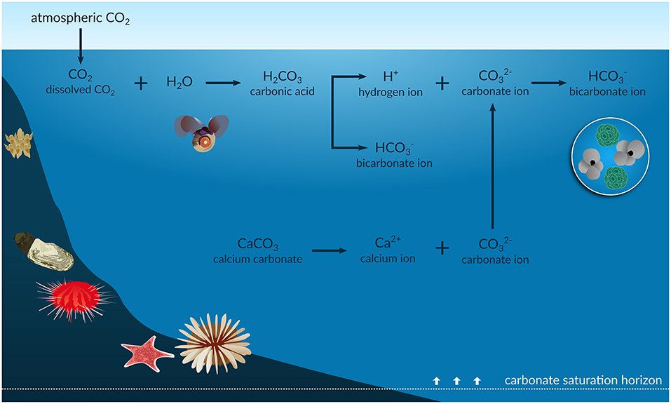
\n", "|:--:|\n", "|Infographic of the ocean acidification process, Source: frontiersin.org|\n", "\n", "First, we initialize the chemical system with aqueous, gaseous, and calcite phases." ] }, { "cell_type": "code", "execution_count": 1, "metadata": { "lines_to_next_cell": 1 }, "outputs": [], "source": [ "from reaktoro import *\n", "\n", "# Create the database\n", "db = SupcrtDatabase(\"supcrtbl\")\n", "\n", "# Create an aqueous phase automatically selecting all species with provided elements\n", "aqueousphase = AqueousPhase(speciate(\"H O C Ca Mg K Cl Na S N\"))\n", "aqueousphase.set(ActivityModelPitzer())\n", "\n", "# Create a gaseous phase\n", "gaseousphase = GaseousPhase(\"CO2(g)\")\n", "gaseousphase.set(ActivityModelPengRobinson())\n", "\n", "# Create a mineral phase\n", "mineral = MineralPhase(\"Calcite\")\n", "\n", "# Create the chemical system\n", "system = ChemicalSystem(db, aqueousphase, gaseousphase, mineral)" ] }, { "cell_type": "markdown", "metadata": {}, "source": [ "Next, the equilibrium specifications, equilibrium conditions, and equilibrium solver for the equilibrium calculations are initialized. To constrain the charge of the chemical state, we need to make it open to the Cl-. Finally, we create aqueous properties to evaluate pH in the forthcoming calculations." ] }, { "cell_type": "code", "execution_count": 2, "metadata": {}, "outputs": [], "source": [ "# Define equilibrium specs\n", "specs = EquilibriumSpecs (system)\n", "specs.temperature()\n", "specs.pressure()\n", "specs.charge()\n", "specs.openTo(\"Cl-\")\n", "\n", "# Define conditions to be satisfied at the chemical equilibrium state\n", "conditions = EquilibriumConditions(specs)\n", "conditions.charge(0.0, \"mol\") # to make sure the mixture is charge neutral\n", "\n", "# Define the equilibrium solver\n", "solver = EquilibriumSolver(specs)\n", "\n", "# Define aqueous properties\n", "aprops = AqueousProps(system)" ] }, { "cell_type": "markdown", "metadata": {}, "source": [ "The functions below define the chemical states corresponding to pure water, rainwater saturated with carbon dioxide, and seawater, respectively:" ] }, { "cell_type": "code", "execution_count": 3, "metadata": {}, "outputs": [], "source": [ "def water():\n", "\n", " state = ChemicalState(system)\n", " state.add(\"H2O(aq)\", 1.0, \"kg\")\n", "\n", " return state\n", "\n", "def rainwater():\n", "\n", " state = ChemicalState(system)\n", " # Rainwater composition\n", " state.set(\"H2O(aq)\", 1.0, \"kg\")\n", " state.set(\"Na+\" , 2.05, \"mg\") # Sodium, 2.05 ppm = 2.05 mg/L ~ 2.05 mg/kgw\n", " state.set(\"K+\" , 0.35, \"mg\") # Potassium\n", " state.set(\"Ca+2\" , 1.42, \"mg\") # Calcium\n", " state.set(\"Mg+2\" , 0.39, \"mg\") # Magnesium\n", " state.set(\"Cl-\" , 3.47, \"mg\") # Chloride\n", " state.set(\"SO4-2\" , 2.19, \"mg\")\n", " state.set(\"NO3-\" , 0.27, \"mg\")\n", " state.set(\"NH4+\" , 0.41, \"mg\")\n", " state.set(\"CO2(aq)\", 0.36, \"mol\") # rainwater is saturated with CO2\n", "\n", " return state\n", "\n", "def seawater():\n", "\n", " state = ChemicalState(system)\n", " # Seawater composition\n", " state.setTemperature(25, \"celsius\")\n", " state.setPressure(1.0, \"bar\")\n", " state.add(\"H2O(aq)\", 1.0, \"kg\")\n", " state.add(\"Ca+2\" , 412.3, \"mg\")\n", " state.add(\"Mg+2\" , 1290.0, \"mg\")\n", " state.add(\"Na+\" , 10768.0, \"mg\")\n", " state.add(\"K+\" , 399.1, \"mg\")\n", " state.add(\"Cl-\" , 19353.0, \"mg\")\n", " state.add(\"HCO3-\" , 141.7, \"mg\")\n", " state.add(\"SO4-2\" , 2712.0, \"mg\")\n", "\n", " return state" ] }, { "cell_type": "markdown", "metadata": {}, "source": [ "## Solubility of calcite for different temperatures and pressures\n", "\n", "To calculate the solubility of calcite in a given brine, we define the function `solubility_of_calcite()`, which calculates the pH of the aqueous solution along with the amount of calcite dissolved in it. As the names suggest, the instances of `pandas.DataFrame`, i.e., `df_water` and `df_rainwater`, correspond to the results of chemical equilibrium calculations for water and rainwater, respectively." ] }, { "cell_type": "code", "execution_count": 4, "metadata": {}, "outputs": [], "source": [ "import pandas as pd\n", "df_water = pd.DataFrame(columns=[\"T\", \"P\", \"pH\", \"deltaCalcite\"])\n", "df_rainwater = pd.DataFrame(columns=[\"T\", \"P\", \"pH\", \"deltaCalcite\"])\n", "\n", "# Initial amount of calcite\n", "n0Calcite = 10.0\n", "\n", "def solubility_of_calcite(state, T, P, tag):\n", "\n", " conditions.temperature(T, \"celsius\")\n", " conditions.pressure(P, \"bar\")\n", "\n", " # Equilibrate the solution with given initial chemical state and desired conditions at equilibrium\n", " res = solver.solve(state, conditions)\n", "\n", " # Check calculation succeeded\n", " assert res.succeeded()\n", "\n", " # Update aqueous properties\n", " aprops.update(state)\n", "\n", " # Fetch the amount of final calcite in the equilibrium state\n", " nCalcite = float(state.speciesAmount(\"Calcite\"))\n", "\n", " if tag == \"water\":\n", " df_water.loc[len(df_water)] = [T, P, float(aprops.pH()), n0Calcite - nCalcite]\n", " elif tag == \"rainwater\":\n", " df_rainwater.loc[len(df_rainwater)] = [T, P, float(aprops.pH()), n0Calcite - nCalcite]" ] }, { "cell_type": "markdown", "metadata": {}, "source": [ "Next, we initialize the array of temperatures from 20 °C till 90 °C and pressures P = 1, 10, 100 bars and perform solubility calculations for water and rainwater." ] }, { "cell_type": "code", "execution_count": 5, "metadata": { "collapsed": false, "jupyter": { "outputs_hidden": false } }, "outputs": [], "source": [ "import numpy as np\n", "temperatures = np.arange(20.0, 91.0, 5.0) # in celsius\n", "pressures = np.array([1, 10, 100]) # in bar\n", "\n", "state = water()\n", "state.set(\"Calcite\", n0Calcite, \"mol\")\n", "[solubility_of_calcite(state, T, P, \"water\") for P in pressures for T in temperatures];\n", "\n", "state = rainwater()\n", "state.set(\"Calcite\", n0Calcite, \"mol\")\n", "[solubility_of_calcite(state, T, P, \"rainwater\") for P in pressures for T in temperatures];" ] }, { "cell_type": "markdown", "metadata": {}, "source": [ "Let us check that the calcite solubility determined for 25 °C and 1 bar actually corresponds to the values from Wikipedia, i.e., the solubility in water is 0.013 g/L (25 °C). In the following, we use 100.0869 g/mol as the molar mass of calcite:" ] }, { "cell_type": "code", "execution_count": 6, "metadata": {}, "outputs": [ { "name": "stdout", "output_type": "stream", "text": [ "Solubility of calcite in water equals to 0.116 mmol/kgw = ... = 0.012 g/L\n" ] } ], "source": [ "# Fetch Calcite solubility for T = 25 celsius and P = 1 bar\n", "deltaCalcite = df_water[(df_water['P']== 1.0) & (df_water['T'] == 25.0)]['deltaCalcite'].iloc[0]\n", "print(f\"Solubility of calcite in water equals to {1e3*deltaCalcite:.3f} \"\n", " f\"mmol/kgw = ... = {deltaCalcite * 0.1000869 * 1e3:.3f} g/L\")" ] }, { "cell_type": "markdown", "metadata": {}, "source": [ "In the case of pure water, therefore, about 0.116 mmol of calcite will dissolve. This dissolved quantity is independent of the initial quantity value used for calcite (provided it exceeds the solubility limit)." ] }, { "attachments": {}, "cell_type": "markdown", "metadata": {}, "source": [ "We plot below the solubility of calcite in water and in CO2-saturated rainwater at 1 bar:" ] }, { "cell_type": "code", "execution_count": 7, "metadata": {}, "outputs": [ { "data": { "text/html": [ " \n", " " ] }, "metadata": {}, "output_type": "display_data" }, { "data": { "application/vnd.plotly.v1+json": { "config": { "plotlyServerURL": "https://plot.ly" }, "data": [ { "mode": "lines+markers", "name": "water", "type": "scatter", "x": [ 20, 25, 30, 35, 40, 45, 50, 55, 60, 65, 70, 75, 80, 85, 90 ], "y": [ 0.00011158823615886604, 0.00011570047996301014, 0.00011972408103488874, 0.00012367519575384733, 0.0001275552374409017, 0.00013135428968880092, 0.00013505431693694447, 0.00013863203597885843, 0.000142061353292533, 0.0001453153397648066, 0.00014836775636162258, 0.00015119417140851965, 0.00015377273588690343, 0.0001560846777781677, 0.00015811458118619726 ] }, { "mode": "lines+markers", "name": "rainwater", "type": "scatter", "x": [ 20, 25, 30, 35, 40, 45, 50, 55, 60, 65, 70, 75, 80, 85, 90 ], "y": [ 0.009323169417667643, 0.008522299561253277, 0.007791197320043963, 0.007124176727096199, 0.006515834973541246, 0.005961098395209419, 0.005455245064966974, 0.004993910738818386, 0.004573084312124109, 0.004189093024448809, 0.003838585323334698, 0.0035185096398198112, 0.0032260920591884457, 0.002958815084930677, 0.0027143962327205173 ] } ], "layout": { "template": { "data": { "scatter": [ { "line": { "width": 4 }, "marker": { "size": 10, "symbol": "circle" }, "type": "scatter" } ] }, "layout": { "colorway": [ "#4C78A8", "#F58518", "#E45756", "#72B7B2", "#54A24B", "#EECA3B", "#B279A2", "#FF9DA6", "#9D755D", "#BAB0AC" ], "font": { "color": "#2e2e2e", "family": "Arial", "size": 16 }, "legend": { "title": { "text": "" } }, "margin": { "b": 100, "l": 100, "pad": 5, "r": 100, "t": 100 }, "paper_bgcolor": "#f7f7f7", "plot_bgcolor": "#f7f7f7", "title": { "font": { "color": "#636363", "size": 24 }, "x": 0, "xref": "paper", "yanchor": "middle", "yref": "paper" }, "xaxis": { "exponentformat": "power", "showexponent": "last", "title": { "font": { "size": 20 } }, "zerolinecolor": "#2e2e2e", "zerolinewidth": 0 }, "yaxis": { "exponentformat": "power", "showexponent": "last", "title": { "font": { "size": 20 } }, "zerolinecolor": "#2e2e2e", "zerolinewidth": 0 } } }, "title": { "text": "CALCITE SOLUBILITY IN WATER AND
CO2-SATURATED RAINWATER AT 1 BAR" }, "xaxis": { "title": { "text": "Temperature [°C]" } }, "yaxis": { "title": { "text": "Calcite Solubility [mol/kgw]" } } } }, "text/html": [ "
" ] }, "metadata": {}, "output_type": "display_data" } ], "source": [ "from reaktplot import *\n", "\n", "df_water_P1 = df_water[df_water['P'] == 1.0]\n", "df_rainwater_P1 = df_rainwater[df_rainwater['P'] == 1.0]\n", "\n", "fig = Figure()\n", "fig.title(\"CALCITE SOLUBILITY IN WATER AND
CO2-SATURATED RAINWATER AT 1 BAR\")\n", "fig.xaxisTitle('Temperature [°C]')\n", "fig.yaxisTitle('Calcite Solubility [mol/kgw]')\n", "fig.drawLineWithMarkers(df_water_P1[\"T\"], df_water_P1[\"deltaCalcite\"], name=\"water\")\n", "fig.drawLineWithMarkers(df_rainwater_P1[\"T\"], df_rainwater_P1[\"deltaCalcite\"], name=\"rainwater\")\n", "\n", "fig.show()" ] }, { "cell_type": "markdown", "metadata": {}, "source": [ "From this plot, it can be seen that calcium carbonate has very low solubility in pure water, but higher solubility in rainwater saturated with carbon dioxide. This is due to the formation of more soluble calcium bicarbonate. The solubilities on different scales and for different pressures are shown below. It can be seen that with increasing pressure, the solubility of calcium carbonate increases." ] }, { "cell_type": "code", "execution_count": 8, "metadata": {}, "outputs": [ { "data": { "application/vnd.plotly.v1+json": { "config": { "plotlyServerURL": "https://plot.ly" }, "data": [ { "mode": "lines+markers", "name": "1 bar", "type": "scatter", "x": [ 20, 25, 30, 35, 40, 45, 50, 55, 60, 65, 70, 75, 80, 85, 90 ], "y": [ 0.00011158823615886604, 0.00011570047996301014, 0.00011972408103488874, 0.00012367519575384733, 0.0001275552374409017, 0.00013135428968880092, 0.00013505431693694447, 0.00013863203597885843, 0.000142061353292533, 0.0001453153397648066, 0.00014836775636162258, 0.00015119417140851965, 0.00015377273588690343, 0.0001560846777781677, 0.00015811458118619726 ] }, { "mode": "lines+markers", "name": "10 bar", "type": "scatter", "x": [ 20, 25, 30, 35, 40, 45, 50, 55, 60, 65, 70, 75, 80, 85, 90 ], "y": [ 0.0001126295222757534, 0.00011673088419428268, 0.00012074363647052166, 0.00012468450065483694, 0.00012855526722788113, 0.00013234623828850545, 0.00013603946836759917, 0.00013961166583165152, 0.0001430366579491249, 0.00014628739050337458, 0.0001493374729424346, 0.0001521623121103488, 0.0001547398984076409, 0.00015705130837062597, 0.00015908098779782165 ] }, { "mode": "lines+markers", "name": "100 bar", "type": "scatter", "x": [ 20, 25, 30, 35, 40, 45, 50, 55, 60, 65, 70, 75, 80, 85, 90 ], "y": [ 0.0001235536066666043, 0.0001275202353170357, 0.0001313990321669678, 0.00013521271955418968, 0.0001389671356371025, 0.0001426549677212563, 0.00014625929939171556, 0.00014975681597206858, 0.0001531205600073804, 0.00015632218661387753, 0.00015933372309362426, 0.00016212887109468, 0.00016468391676305316, 0.0001669783152067339, 0.00016899502668188404 ] } ], "layout": { "template": { "data": { "scatter": [ { "line": { "width": 4 }, "marker": { "size": 10, "symbol": "circle" }, "type": "scatter" } ] }, "layout": { "colorway": [ "#4C78A8", "#F58518", "#E45756", "#72B7B2", "#54A24B", "#EECA3B", "#B279A2", "#FF9DA6", "#9D755D", "#BAB0AC" ], "font": { "color": "#2e2e2e", "family": "Arial", "size": 16 }, "legend": { "title": { "text": "" } }, "margin": { "b": 100, "l": 100, "pad": 5, "r": 100, "t": 100 }, "paper_bgcolor": "#f7f7f7", "plot_bgcolor": "#f7f7f7", "title": { "font": { "color": "#636363", "size": 24 }, "x": 0, "xref": "paper", "yanchor": "middle", "yref": "paper" }, "xaxis": { "exponentformat": "power", "showexponent": "last", "title": { "font": { "size": 20 } }, "zerolinecolor": "#2e2e2e", "zerolinewidth": 0 }, "yaxis": { "exponentformat": "power", "showexponent": "last", "title": { "font": { "size": 20 } }, "zerolinecolor": "#2e2e2e", "zerolinewidth": 0 } } }, "title": { "text": "CALCITE SOLUBILITY IN WATER" }, "xaxis": { "title": { "text": "Temperature [°C]" } }, "yaxis": { "title": { "text": "Calcite Solubility [mol/kgw]" } } } }, "text/html": [ "
" ] }, "metadata": {}, "output_type": "display_data" }, { "data": { "application/vnd.plotly.v1+json": { "config": { "plotlyServerURL": "https://plot.ly" }, "data": [ { "mode": "lines+markers", "name": "1 bar", "type": "scatter", "x": [ 20, 25, 30, 35, 40, 45, 50, 55, 60, 65, 70, 75, 80, 85, 90 ], "y": [ 0.009323169417667643, 0.008522299561253277, 0.007791197320043963, 0.007124176727096199, 0.006515834973541246, 0.005961098395209419, 0.005455245064966974, 0.004993910738818386, 0.004573084312124109, 0.004189093024448809, 0.003838585323334698, 0.0035185096398198112, 0.0032260920591884457, 0.002958815084930677, 0.0027143962327205173 ] }, { "mode": "lines+markers", "name": "10 bar", "type": "scatter", "x": [ 20, 25, 30, 35, 40, 45, 50, 55, 60, 65, 70, 75, 80, 85, 90 ], "y": [ 0.02154037090572203, 0.02029426297342951, 0.0185719038338803, 0.01699813323613597, 0.015560346358526544, 0.014246951164128774, 0.013047259185343663, 0.011951413072440076, 0.010950340739022124, 0.010035708522080355, 0.009199880194712406, 0.008435870230808717, 0.007737301009834496, 0.007098356467814426, 0.006513740358920828 ] }, { "mode": "lines+markers", "name": "100 bar", "type": "scatter", "x": [ 20, 25, 30, 35, 40, 45, 50, 55, 60, 65, 70, 75, 80, 85, 90 ], "y": [ 0.02333365917518293, 0.022442103603474095, 0.02150554612934208, 0.02054000646897869, 0.019558969520787173, 0.018573736251516593, 0.01759371310473412, 0.016626662769823497, 0.015678919040228223, 0.01475557544203454, 0.013860649204051612, 0.012997229364632545, 0.012167602353288842, 0.01137336499162167, 0.010615525620790933 ] } ], "layout": { "template": { "data": { "scatter": [ { "line": { "width": 4 }, "marker": { "size": 10, "symbol": "circle" }, "type": "scatter" } ] }, "layout": { "colorway": [ "#4C78A8", "#F58518", "#E45756", "#72B7B2", "#54A24B", "#EECA3B", "#B279A2", "#FF9DA6", "#9D755D", "#BAB0AC" ], "font": { "color": "#2e2e2e", "family": "Arial", "size": 16 }, "legend": { "title": { "text": "" } }, "margin": { "b": 100, "l": 100, "pad": 5, "r": 100, "t": 100 }, "paper_bgcolor": "#f7f7f7", "plot_bgcolor": "#f7f7f7", "title": { "font": { "color": "#636363", "size": 24 }, "x": 0, "xref": "paper", "yanchor": "middle", "yref": "paper" }, "xaxis": { "exponentformat": "power", "showexponent": "last", "title": { "font": { "size": 20 } }, "zerolinecolor": "#2e2e2e", "zerolinewidth": 0 }, "yaxis": { "exponentformat": "power", "showexponent": "last", "title": { "font": { "size": 20 } }, "zerolinecolor": "#2e2e2e", "zerolinewidth": 0 } } }, "title": { "text": "CALCITE SOLUBILITY IN CO2-SATURATED RAINWATER" }, "xaxis": { "title": { "text": "Temperature [°C]" } }, "yaxis": { "title": { "text": "Calcite Solubility [mol/kgw]" } } } }, "text/html": [ "
" ] }, "metadata": {}, "output_type": "display_data" } ], "source": [ "from reaktplot import *\n", "\n", "fig1 = Figure()\n", "fig1.title(\"CALCITE SOLUBILITY IN WATER\")\n", "fig1.xaxisTitle('Temperature [°C]')\n", "fig1.yaxisTitle('Calcite Solubility [mol/kgw]')\n", "\n", "for P in pressures:\n", " df_water_P = df_water[df_water['P'] == P]\n", " fig1.drawLineWithMarkers(df_water_P[\"T\"], df_water_P[\"deltaCalcite\"], name=f'{P} bar')\n", "\n", "fig2 = Figure()\n", "fig2.title(\"CALCITE SOLUBILITY IN CO2-SATURATED RAINWATER\")\n", "fig2.xaxisTitle('Temperature [°C]')\n", "fig2.yaxisTitle('Calcite Solubility [mol/kgw]')\n", "\n", "for P in pressures:\n", " df_rainwater_P = df_rainwater[df_water['P'] == P]\n", " fig2.drawLineWithMarkers(df_rainwater_P[\"T\"], df_rainwater_P[\"deltaCalcite\"], name=f'{P} bar')\n", "\n", "fig1.show()\n", "fig2.show()" ] }, { "cell_type": "markdown", "metadata": {}, "source": [ "### Solubility of calcite in the seawater with increasing levels of CO2\n", "\n", "Subsequent auxiliary variables are defined to store the initial amount of CO2 and its incremental amount in the calculation sequence. At each iteration of the following loop, CO2 is added to the seawater and the system is rebalanced.\n", "The amount of carbon dioxide added and the corresponding pH value are recorded in a `pandas.DataFrame`." ] }, { "cell_type": "code", "execution_count": 9, "metadata": { "collapsed": false, "jupyter": { "outputs_hidden": false } }, "outputs": [], "source": [ "co2_0 = 0.0\n", "co2_delta = 2.0 # in mmol\n", "nsteps = 50\n", "\n", "df_seawater = pd.DataFrame(columns=[\"amountCO2\", \"pH\", \"deltaCalcite\"])\n", "\n", "T = 25\n", "P = 1\n", "\n", "for i in range(nsteps):\n", "\n", " # Initial amount of calcite\n", " n0Calcite = 10.0\n", "\n", " conditions.temperature(T, \"celsius\")\n", " conditions.pressure(P, \"bar\")\n", "\n", " # Add more CO2 to the problem\n", " state = seawater()\n", " state.set(\"CO2(g)\", co2_0, \"mmol\")\n", " state.set(\"O2(aq)\", 1.0e-9, \"mol\") # this small amount of O2(aq) is needed to avoid convergence failure in the computation below!\n", "\n", " # Equilibrate the solution given by the chemical state and conditions\n", " res = solver.solve(state, conditions)\n", " \n", " # Check calculation succeeded\n", " assert res.succeeded(), f\"The calculation failed at step #{i}\"\n", "\n", " # Add `n0Calcite` amount of calcite\n", " state.set(\"Calcite\", n0Calcite, \"mol\")\n", "\n", " # Equilibrate solution with added calcite\n", " res = solver.solve(state, conditions)\n", "\n", " # Check calculation succeeded\n", " assert res.succeeded(), f\"The calculation failed at step #{i}\"\n", "\n", " # Update aqueous properties\n", " aprops.update(state)\n", "\n", " # Fetch the amount of final calcite in the equilibrium state\n", " nCalcite = float(state.speciesAmount(\"Calcite\"))\n", "\n", " # Update CO2 amount\n", " co2_0 += co2_delta\n", "\n", " # Append new calculated value to the dataframe\n", " df_seawater.loc[len(df_seawater)] = [co2_0, float(aprops.pH()), n0Calcite - nCalcite]" ] }, { "cell_type": "markdown", "metadata": {}, "source": [ "To analyze the results obtained, the pH and calcite solubility are plotted as a function of the amount of CO2 added to the seawater." ] }, { "cell_type": "code", "execution_count": null, "metadata": {}, "outputs": [ { "data": { "application/vnd.plotly.v1+json": { "config": { "plotlyServerURL": "https://plot.ly" }, "data": [ { "mode": "lines+markers", "name": "", "type": "scatter", "x": [ 2, 4, 6, 8, 10, 12, 14, 16, 18, 20, 22, 24, 26, 28, 30, 32, 34, 36, 38, 40, 42, 44, 46, 48, 50, 52, 54, 56, 58, 60, 62, 64, 66, 68, 70, 72, 74, 76, 78, 80, 82, 84, 86, 88, 90, 92, 94, 96, 98, 100 ], "y": [ 7.427740716810793, 6.9948062638836, 6.790896669318783, 6.659625444741551, 6.563922150858276, 6.489134033470023, 6.42802221510274, 6.376504898122313, 6.332065793563736, 6.293049964330791, 6.258313956865966, 6.22703638662136, 6.198608345663321, 6.172566532429699, 6.148550631793111, 6.12627514324458, 6.1055101743094236, 6.086067993029829, 6.067793392267042, 6.050556643609286, 6.034248251472249, 6.018774984346083, 6.01204877119714, 6.012048771197121, 6.012048771197107, 6.012048771197111, 6.0120487711971045, 6.012048771197114, 6.012048771197112, 6.01204877119711, 6.012048771197096, 6.012048771197109, 6.012048771197107, 6.0120487711971, 6.0120487711971125, 6.012048771197108, 6.012048771197105, 6.012048771199196, 6.012048771199187, 6.0120487711991935, 6.012048771199184, 6.012048771199187, 6.012048771199191, 6.012048771199189, 6.012048771199187, 6.012048771199191, 6.012048771199182, 6.012048771199187, 6.012048771199187, 6.012048771199182 ] } ], "layout": { "height": 500, "template": { "data": { "scatter": [ { "line": { "width": 4 }, "marker": { "size": 10, "symbol": "circle" }, "type": "scatter" } ] }, "layout": { "colorway": [ "#4C78A8", "#F58518", "#E45756", "#72B7B2", "#54A24B", "#EECA3B", "#B279A2", "#FF9DA6", "#9D755D", "#BAB0AC" ], "font": { "color": "#2e2e2e", "family": "Arial", "size": 16 }, "legend": { "title": { "text": "" } }, "margin": { "b": 100, "l": 100, "pad": 5, "r": 100, "t": 100 }, "paper_bgcolor": "#f7f7f7", "plot_bgcolor": "#f7f7f7", "title": { "font": { "color": "#636363", "size": 24 }, "x": 0, "xref": "paper", "yanchor": "middle", "yref": "paper" }, "xaxis": { "title": { "font": { "size": 20 } }, "zerolinecolor": "#2e2e2e", "zerolinewidth": 0 }, "yaxis": { "title": { "font": { "size": 20 } }, "zerolinecolor": "#2e2e2e", "zerolinewidth": 0 } } }, "title": { "text": "PH DEPENDENCE ON AMOUNT OF
ADDED CO2 TO THE SEAWATER" }, "xaxis": { "title": { "text": "CO2 [mmol]" } }, "yaxis": { "title": { "text": "pH" } } } }, "text/html": [ "
" ] }, "metadata": {}, "output_type": "display_data" }, { "data": { "application/vnd.plotly.v1+json": { "config": { "plotlyServerURL": "https://plot.ly" }, "data": [ { "mode": "lines+markers", "name": "", "type": "scatter", "x": [ 2, 4, 6, 8, 10, 12, 14, 16, 18, 20, 22, 24, 26, 28, 30, 32, 34, 36, 38, 40, 42, 44, 46, 48, 50, 52, 54, 56, 58, 60, 62, 64, 66, 68, 70, 72, 74, 76, 78, 80, 82, 84, 86, 88, 90, 92, 94, 96, 98, 100 ], "y": [ 0, 0.001410708409135708, 0.002580660713721983, 0.0035554179235575134, 0.004395432764191298, 0.00513706787855206, 0.0058036499745295345, 0.006410982628224815, 0.006970259052577532, 0.007489699103135905, 0.007975521453138512, 0.008432548893672731, 0.008864600705436487, 0.009274755923778244, 0.009665535300097616, 0.01003903034868614, 0.010396996952277249, 0.010740924619376813, 0.011072088636334243, 0.011391589960103587, 0.011700386166239696, 0.011999315764773755, 0.012131089891385116, 0.012131089891386893, 0.012131089891385116, 0.012131089891386893, 0.012131089891386893, 0.012131089891386893, 0.012131089891385116, 0.012131089891386893, 0.012131089891386893, 0.012131089891386893, 0.012131089891386893, 0.012131089891386893, 0.012131089891386893, 0.012131089891386893, 0.012131089891386893, 0.012131089891411762, 0.012131089891411762, 0.012131089891411762, 0.012131089891411762, 0.012131089891411762, 0.012131089891411762, 0.012131089891411762, 0.012131089891411762, 0.012131089891411762, 0.012131089891411762, 0.012131089891411762, 0.012131089891411762, 0.012131089891411762 ] } ], "layout": { "height": 500, "template": { "data": { "scatter": [ { "line": { "width": 4 }, "marker": { "size": 10, "symbol": "circle" }, "type": "scatter" } ] }, "layout": { "colorway": [ "#4C78A8", "#F58518", "#E45756", "#72B7B2", "#54A24B", "#EECA3B", "#B279A2", "#FF9DA6", "#9D755D", "#BAB0AC" ], "font": { "color": "#2e2e2e", "family": "Arial", "size": 16 }, "legend": { "title": { "text": "" } }, "margin": { "b": 100, "l": 100, "pad": 5, "r": 100, "t": 100 }, "paper_bgcolor": "#f7f7f7", "plot_bgcolor": "#f7f7f7", "title": { "font": { "color": "#636363", "size": 24 }, "x": 0, "xref": "paper", "yanchor": "middle", "yref": "paper" }, "xaxis": { "title": { "font": { "size": 20 } }, "zerolinecolor": "#2e2e2e", "zerolinewidth": 0 }, "yaxis": { "title": { "font": { "size": 20 } }, "zerolinecolor": "#2e2e2e", "zerolinewidth": 0 } } }, "title": { "text": "THE EFFECT OF CO2 CONTENT IN SEAWATER
ON CALCITE SOLUBILITY" }, "xaxis": { "title": { "text": "CO2 [mmol]" } }, "yaxis": { "title": { "text": "Calcite Solubility [mol/kgw]" } } } }, "text/html": [ "
" ] }, "metadata": {}, "output_type": "display_data" } ], "source": [ "fig1 = Figure()\n", "fig1.title(\"PH DEPENDENCE ON AMOUNT OF
ADDED CO2 TO THE SEAWATER\")\n", "fig1.xaxisTitle('CO2 [mmol]')\n", "fig1.yaxisTitle('pH')\n", "fig1.drawLineWithMarkers(df_seawater[\"amountCO2\"], df_seawater[\"pH\"], name=\"\")\n", "\n", "fig2 = Figure()\n", "fig2.title(\"THE EFFECT OF CO2 CONTENT IN SEAWATER
ON CALCITE SOLUBILITY\")\n", "fig2.xaxisTitle('CO2 [mmol]')\n", "fig2.yaxisTitle('Calcite Solubility [mol/kgw]')\n", "fig2.drawLineWithMarkers(df_seawater[\"amountCO2\"], df_seawater[\"deltaCalcite\"], name=\"\")\n", "\n", "fig1.height(500)\n", "fig2.height(500)\n", "\n", "fig1.show()\n", "fig2.show()" ] }, { "cell_type": "markdown", "metadata": {}, "source": [ "Below 45 mmol CO2, the seawater becomes increasingly acidic with the addition of the gas, which increases the solubility of the calcite. However, once the saturation point is reached, no more gas can be dissolved in the seawater and the pH remains constant. The solubility of the calcite is also constant from this point on." ] } ], "metadata": { "kernelspec": { "display_name": "Python 3.9.9 ('reaktoro-jupyter-book')", "language": "python", "name": "python3" }, "language_info": { "codemirror_mode": { "name": "ipython", "version": 3 }, "file_extension": ".py", "mimetype": "text/x-python", "name": "python", "nbconvert_exporter": "python", "pygments_lexer": "ipython3", "version": "3.11.5" }, "vscode": { "interpreter": { "hash": "e4e8b2f3ae27709963f14fd23a6560d362beea55eaec742263828e04d814e23c" } } }, "nbformat": 4, "nbformat_minor": 4 }