 [](https://cran.r-project.org/package=potential)
[](https://github.com/riatelab/potential/actions/workflows/R-CMD-check.yaml)
[](https://app.codecov.io/gh/riatelab/potential)
[](https://www.repostatus.org/#active)
This package provides functions to compute the potential model as
defined by Stewart (1941). Several options are available to customize
the model, for example it is possible to fine-tune the distance friction
functions or to use custom distance matrices. Some computations are
parallelized to improve their efficiency.
- [**Website**](https://riatelab.github.io/potential/)
- [**Vignette**](https://riatelab.github.io/potential/articles/potential.html)
- [**Blog post**](https://rgeomatic.hypotheses.org/2023)
## Installation
You can install the released version of `potential` from
[CRAN](https://CRAN.R-project.org/package=potential) with:
``` r
install.packages("potential")
```
You can install the development version of `potential` from GitHub with:
``` r
# install.packages("remotes")
remotes::install_github("riatelab/potential")
```
## Demo
``` r
library(mapsf)
library(potential)
# Display the spatial interaction function
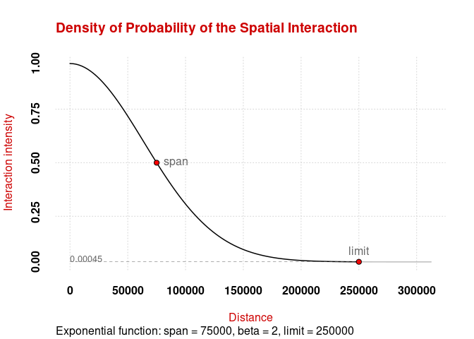
plot_inter(fun = "e", span = 75000, beta = 2, limit = 250000)
```
``` r
# create a regular grid
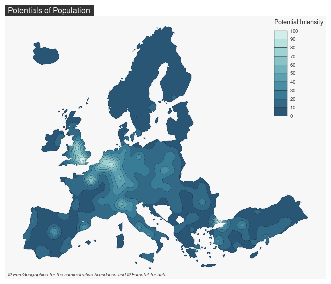
y <- create_grid(x = n3_poly, res = 20000)
# compute potentials
pot <- mcpotential(
x = n3_pt, y = y,
var = "POP19",
fun = "e", span = 75000,
beta = 2, limit = 250000,
ncl = 2
)
# Define potential according to the maximum value
y$pot <- pot / max(pot) * 100
# create equipotential areas
bks <- seq(0, 100, length.out = 11)
equipot <- equipotential(y, var = "pot", breaks = bks, mask = n3_poly)
# map potentials
mf_map(x = equipot, var = "min", type = "choro",
breaks = bks,
pal = hcl.colors(10, 'Teal'),
border = "#121725",
leg_val_rnd = 0,
lwd = .2,
leg_pos = "topright",
leg_title = "Potential Intensity")
mf_title(txt = "Potentials of Population")
mf_credits(txt = "© EuroGeographics for the administrative boundaries and © Eurostat for data")
```
## Note
This package provides access to the revamped potential-related functions
initially offered by
[`SpatialPosition`](https://CRAN.R-project.org/package=SpatialPosition).
## References
[](https://cran.r-project.org/package=potential)
[](https://github.com/riatelab/potential/actions/workflows/R-CMD-check.yaml)
[](https://app.codecov.io/gh/riatelab/potential)
[](https://www.repostatus.org/#active)
This package provides functions to compute the potential model as
defined by Stewart (1941). Several options are available to customize
the model, for example it is possible to fine-tune the distance friction
functions or to use custom distance matrices. Some computations are
parallelized to improve their efficiency.
- [**Website**](https://riatelab.github.io/potential/)
- [**Vignette**](https://riatelab.github.io/potential/articles/potential.html)
- [**Blog post**](https://rgeomatic.hypotheses.org/2023)
## Installation
You can install the released version of `potential` from
[CRAN](https://CRAN.R-project.org/package=potential) with:
``` r
install.packages("potential")
```
You can install the development version of `potential` from GitHub with:
``` r
# install.packages("remotes")
remotes::install_github("riatelab/potential")
```
## Demo
``` r
library(mapsf)
library(potential)
# Display the spatial interaction function
plot_inter(fun = "e", span = 75000, beta = 2, limit = 250000)
```

``` r
# create a regular grid
y <- create_grid(x = n3_poly, res = 20000)
# compute potentials
pot <- mcpotential(
x = n3_pt, y = y,
var = "POP19",
fun = "e", span = 75000,
beta = 2, limit = 250000,
ncl = 2
)
# Define potential according to the maximum value
y$pot <- pot / max(pot) * 100
# create equipotential areas
bks <- seq(0, 100, length.out = 11)
equipot <- equipotential(y, var = "pot", breaks = bks, mask = n3_poly)
# map potentials
mf_map(x = equipot, var = "min", type = "choro",
breaks = bks,
pal = hcl.colors(10, 'Teal'),
border = "#121725",
leg_val_rnd = 0,
lwd = .2,
leg_pos = "topright",
leg_title = "Potential Intensity")
mf_title(txt = "Potentials of Population")
mf_credits(txt = "© EuroGeographics for the administrative boundaries and © Eurostat for data")
```

## Note
This package provides access to the revamped potential-related functions
initially offered by
[`SpatialPosition`](https://CRAN.R-project.org/package=SpatialPosition).
## References