# Tanaka  [](https://CRAN.R-project.org/package=tanaka)
[](https://github.com/riatelab/tanaka/actions)
[](https://app.codecov.io/github/riatelab/tanaka?branch=master)

[](https://www.repostatus.org/#active)
Also called "relief contours method", "illuminated contour method" or "shaded
contour lines method", the Tanaka method[1](#fn1) enhances the representation of topography
on a map by using shaded contour lines. The result is a 3D-like map.
This package is a simplified implementation of the Tanaka method, north-west white contours represent
illuminated topography and south-east black contours represent shaded topography.
Even if the results are quite satisfactory, a more refined method could be used
based on the Kennelly and Kimerling's paper[2](#fn2).
`tanaka` is a small package with two functions:
- `tanaka()` uses a `terra` object and displays the map directly;
- `tanaka_contour()` builds the isopleth polygon layer.
The contour lines creation relies on [`mapiso`](https://github.com/riatelab/mapiso),
spatial manipulation and display rely on [`sf`](https://github.com/r-spatial/sf).
## Installation
* From CRAN
```r
install.packages("tanaka")
```
* Development version on GitHub
```r
require(remotes)
install_github("riatelab/tanaka")
```
## Demo
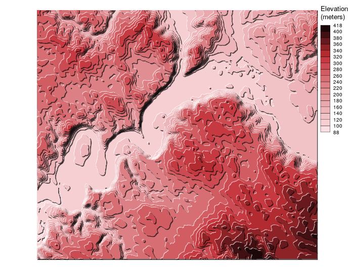
* This example is based on the dataset shipped within the package.
```r
library(tanaka)
library(terra)
ras <- rast(system.file("tif/elev.tif", package = "tanaka"))
tanaka(ras, breaks = seq(80,400,20),
legend.pos = "topright", legend.title = "Elevation\n(meters)")
```
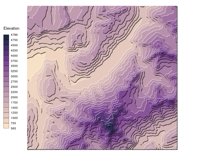
* This example is based on an elevation raster downloaded via
[`elevatr`](https://github.com/jhollist/elevatr).
```r
library(tanaka)
library(elevatr)
library(terra)
# use elevatr to get elevation data
ras <- get_elev_raster(locations = data.frame(x = c(6.7, 7), y = c(45.8,46)),
z = 10, prj = "EPSG:4326", clip = "locations")
ras <- rast(ras)
# custom color palette
cols <- c("#F7E1C6", "#EED4C1", "#E5C9BE", "#DCBEBA", "#D3B3B6", "#CAA8B3",
"#C19CAF", "#B790AB", "#AC81A7", "#A073A1", "#95639D", "#885497",
"#7C4692", "#6B3D86", "#573775", "#433266", "#2F2C56", "#1B2847")
# display the map
tanaka(ras, breaks = seq(500,4800,250), col = cols)
```
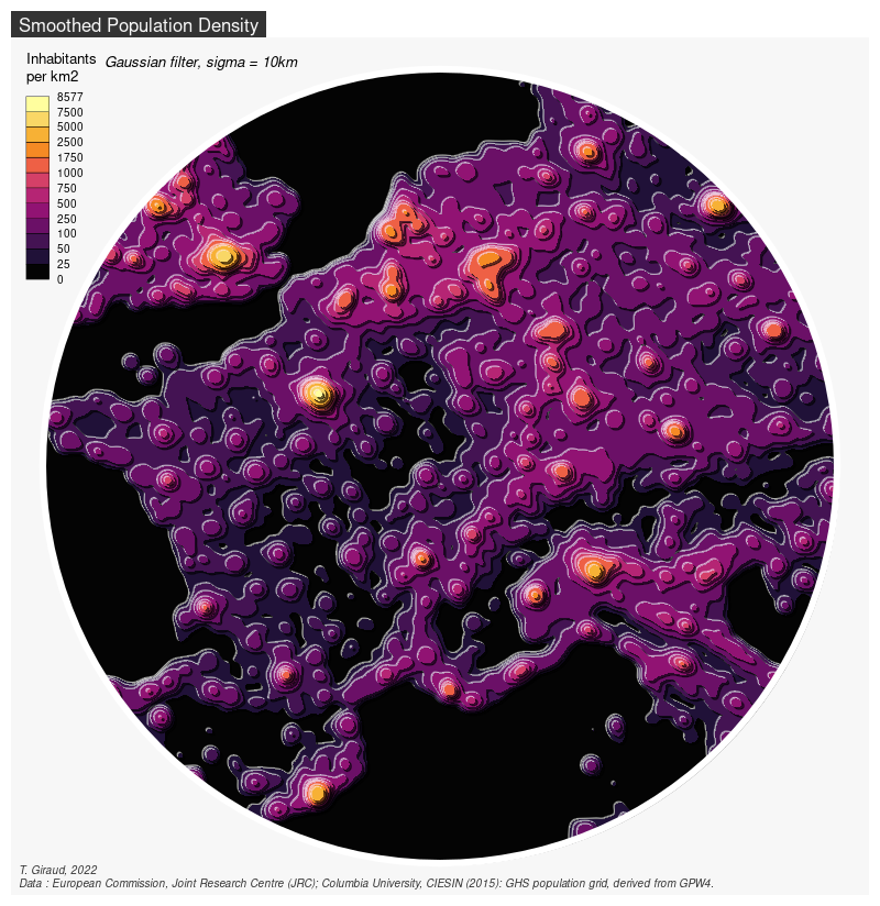
* The last example illustrates the use of tanaka with non-topographical data.
This map is based on the [Global Human Settlement Population Grid](https://ghsl.jrc.ec.europa.eu/ghs_pop.php) (1km).
```r
library(terra)
library(sf)
library(tanaka)
library(mapsf)
# Download
tempzip <- tempfile()
tempfolder <- tempdir()
data_url <- paste0("http://cidportal.jrc.ec.europa.eu/ftp/jrc-opendata/GHSL/",
"GHS_POP_GPW4_GLOBE_R2015A/GHS_POP_GPW42015_GLOBE_R2015A_54009_1k/",
"V1-0/GHS_POP_GPW42015_GLOBE_R2015A_54009_1k_v1_0.zip")
download.file(data_url, tempzip)
unzip(tempzip, exdir = tempfolder)
# Import
pop2015 <- rast(paste0(tempfolder,
"/GHS_POP_GPW42015_GLOBE_R2015A_54009_1k_v1_0/",
"GHS_POP_GPW42015_GLOBE_R2015A_54009_1k_v1_0.tif"))
# Mask raster
center <- st_as_sf(data.frame(x=425483.8, y=5608290),
coords=(c("x","y")),
crs = st_crs(pop2015))
center <- st_buffer(center, dist = 800000)
ras <- crop(pop2015, st_bbox(center)[c(1,3,2,4)])
# Smooth values
mat <- focalMat(x = ras, d = c(10000), type = "Gauss")
rassmooth <- focal(x = ras, w = mat, fun = sum, na.rm = TRUE)
# Map
bks <- c(0,25,50,100,250,500,750,1000,1750,2500,5000, 7500,10000)
mf_export(x = center, filename = "circle.png", width = 800, res = 100)
tanaka(x = rassmooth,
breaks = bks,
mask = center,
col = hcl.colors(n = 12, palette = "Inferno"),
shift = 2500,
add = TRUE,
legend.pos = "topleft",
legend.title = "Inhabitants\nper km2")
mf_map(center, add = TRUE, border = "white", col = NA, lwd = 6)
mf_title(txt = "Smoothed Population Density")
mf_credits(paste0("T. Giraud, 2022\n",
"Data : European Commission, Joint Research Centre (JRC); ",
"Columbia University, CIESIN (2015): GHS population grid, ",
"derived from GPW4."))
text(-250000 ,6420000, "Gaussian filter, sigma = 10km",
adj = 0, font = 3, cex = .8, xpd = TRUE )
dev.off()
```
## Alternative Package
The [`metR` package](https://CRAN.R-project.org/package=metR) allows to draw [Tanaka contours with ggplot2](https://eliocamp.github.io/metR/reference/geom_contour_tanaka.html).
-------------------------------------------
1: Tanaka, K. (1950). The relief contour method of representing topography on maps. *Geographical Review, 40*(3), 444-456.
2: Kennelly, P., & Kimerling, A. J. (2001). Modifications of Tanaka's illuminated contour method. *Cartography and Geographic Information Science, 28*(2), 111-123.
[](https://CRAN.R-project.org/package=tanaka)
[](https://github.com/riatelab/tanaka/actions)
[](https://app.codecov.io/github/riatelab/tanaka?branch=master)

[](https://www.repostatus.org/#active)
Also called "relief contours method", "illuminated contour method" or "shaded
contour lines method", the Tanaka method[1](#fn1) enhances the representation of topography
on a map by using shaded contour lines. The result is a 3D-like map.
This package is a simplified implementation of the Tanaka method, north-west white contours represent
illuminated topography and south-east black contours represent shaded topography.
Even if the results are quite satisfactory, a more refined method could be used
based on the Kennelly and Kimerling's paper[2](#fn2).
`tanaka` is a small package with two functions:
- `tanaka()` uses a `terra` object and displays the map directly;
- `tanaka_contour()` builds the isopleth polygon layer.
The contour lines creation relies on [`mapiso`](https://github.com/riatelab/mapiso),
spatial manipulation and display rely on [`sf`](https://github.com/r-spatial/sf).
## Installation
* From CRAN
```r
install.packages("tanaka")
```
* Development version on GitHub
```r
require(remotes)
install_github("riatelab/tanaka")
```
## Demo
* This example is based on the dataset shipped within the package.
```r
library(tanaka)
library(terra)
ras <- rast(system.file("tif/elev.tif", package = "tanaka"))
tanaka(ras, breaks = seq(80,400,20),
legend.pos = "topright", legend.title = "Elevation\n(meters)")
```

* This example is based on an elevation raster downloaded via
[`elevatr`](https://github.com/jhollist/elevatr).
```r
library(tanaka)
library(elevatr)
library(terra)
# use elevatr to get elevation data
ras <- get_elev_raster(locations = data.frame(x = c(6.7, 7), y = c(45.8,46)),
z = 10, prj = "EPSG:4326", clip = "locations")
ras <- rast(ras)
# custom color palette
cols <- c("#F7E1C6", "#EED4C1", "#E5C9BE", "#DCBEBA", "#D3B3B6", "#CAA8B3",
"#C19CAF", "#B790AB", "#AC81A7", "#A073A1", "#95639D", "#885497",
"#7C4692", "#6B3D86", "#573775", "#433266", "#2F2C56", "#1B2847")
# display the map
tanaka(ras, breaks = seq(500,4800,250), col = cols)
```

* The last example illustrates the use of tanaka with non-topographical data.
This map is based on the [Global Human Settlement Population Grid](https://ghsl.jrc.ec.europa.eu/ghs_pop.php) (1km).
```r
library(terra)
library(sf)
library(tanaka)
library(mapsf)
# Download
tempzip <- tempfile()
tempfolder <- tempdir()
data_url <- paste0("http://cidportal.jrc.ec.europa.eu/ftp/jrc-opendata/GHSL/",
"GHS_POP_GPW4_GLOBE_R2015A/GHS_POP_GPW42015_GLOBE_R2015A_54009_1k/",
"V1-0/GHS_POP_GPW42015_GLOBE_R2015A_54009_1k_v1_0.zip")
download.file(data_url, tempzip)
unzip(tempzip, exdir = tempfolder)
# Import
pop2015 <- rast(paste0(tempfolder,
"/GHS_POP_GPW42015_GLOBE_R2015A_54009_1k_v1_0/",
"GHS_POP_GPW42015_GLOBE_R2015A_54009_1k_v1_0.tif"))
# Mask raster
center <- st_as_sf(data.frame(x=425483.8, y=5608290),
coords=(c("x","y")),
crs = st_crs(pop2015))
center <- st_buffer(center, dist = 800000)
ras <- crop(pop2015, st_bbox(center)[c(1,3,2,4)])
# Smooth values
mat <- focalMat(x = ras, d = c(10000), type = "Gauss")
rassmooth <- focal(x = ras, w = mat, fun = sum, na.rm = TRUE)
# Map
bks <- c(0,25,50,100,250,500,750,1000,1750,2500,5000, 7500,10000)
mf_export(x = center, filename = "circle.png", width = 800, res = 100)
tanaka(x = rassmooth,
breaks = bks,
mask = center,
col = hcl.colors(n = 12, palette = "Inferno"),
shift = 2500,
add = TRUE,
legend.pos = "topleft",
legend.title = "Inhabitants\nper km2")
mf_map(center, add = TRUE, border = "white", col = NA, lwd = 6)
mf_title(txt = "Smoothed Population Density")
mf_credits(paste0("T. Giraud, 2022\n",
"Data : European Commission, Joint Research Centre (JRC); ",
"Columbia University, CIESIN (2015): GHS population grid, ",
"derived from GPW4."))
text(-250000 ,6420000, "Gaussian filter, sigma = 10km",
adj = 0, font = 3, cex = .8, xpd = TRUE )
dev.off()
```

## Alternative Package
The [`metR` package](https://CRAN.R-project.org/package=metR) allows to draw [Tanaka contours with ggplot2](https://eliocamp.github.io/metR/reference/geom_contour_tanaka.html).
-------------------------------------------
1: Tanaka, K. (1950). The relief contour method of representing topography on maps. *Geographical Review, 40*(3), 444-456.
2: Kennelly, P., & Kimerling, A. J. (2001). Modifications of Tanaka's illuminated contour method. *Cartography and Geographic Information Science, 28*(2), 111-123.