[](https://github.com/ropensci/osmplotr/actions/workflows/R-CMD-check.yaml)
[](https://app.codecov.io/gh/ropensci/osmplotr)
[](https://www.repostatus.org/)
[](https://cran.r-project.org/package=osmplotr/)
[](https://cran.r-project.org/package=osmplotr/)
[](https://github.com/ropensci/software-review/issues/27)
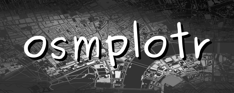
R package to produce visually impressive customisable images of
OpenStreetMap (OSM) data downloaded internally from the [overpass
api](http://overpass-api.de/). The above map was produced directly from
`osmplotr` with no further modification. This `README` briefly
demonstrates the following functionality:
[1. Quick Introduction](#1%20intro)
[2. Installation](#2%20installation)
[3. A Simple Map](#3%20simple%20map)
[4. Highlighting Selected Areas](#4%20highlighting%20areas)
[5. Highlighting Clusters](#5%20highlighting%20clusters)
[6. Highlighting Areas Bounded by Named
Highways](#6%20highlighting%20with%20highways)
[7. Data Surfaces](#7%20data%20surfaces)
[8. Gallery](#8%20gallery)
------------------------------------------------------------------------
## 1. Quick Introduction
But first the easy steps to map making:
1. Specify the bounding box for the desired region
``` r
bbox <- get_bbox (c (-0.15, 51.5, -0.10, 51.52))
```
2. Download the desired data—in this case, all building perimeters.
``` r
dat_B <- extract_osm_objects (key = "building", bbox = bbox)
```
3. Initiate an `osm_basemap` with desired background (`bg`) colour
``` r
map <- osm_basemap (bbox = bbox, bg = "gray20")
```
4. Overlay objects on plot in the desired colour.
``` r
map <- add_osm_objects (map, dat_B, col = "gray40")
```
5. Print the map to graphics device of choice
``` r
print_osm_map (map)
```
------------------------------------------------------------------------
## 2. Installation
First install the package
``` r
install.packages ("osmplotr")
```
or the development version
``` r
devtools::install_github ("ropensci/osmplotr")
```
And then load it in the usual way
``` r
library (osmplotr)
```
------------------------------------------------------------------------
## 3. A Simple Map
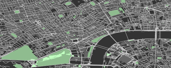
Simple maps can be made by overlaying different kinds of OSM data in
different colours:
``` r
dat_H <- extract_osm_objects (key = "highway", bbox = bbox)
dat_P <- extract_osm_objects (key = "park", bbox = bbox)
dat_G <- extract_osm_objects (key = "landuse", value = "grass", bbox = bbox)
```
``` r
map <- osm_basemap (bbox = bbox, bg = "gray20")
map <- add_osm_objects (map, dat_B, col = "gray40")
map <- add_osm_objects (map, dat_H, col = "gray80")
map <- add_osm_objects (map, dat_P, col = "darkseagreen")
map <- add_osm_objects (map, dat_G, col = "darkseagreen1")
print_osm_map (map)
```
 ------------------------------------------------------------------------
## 4. Highlighting Selected Areas
`osmplotr` is primarily intended as a data visualisation tool,
particularly through enabling selected regions to be highlighted.
Regions can be defined according to simple point boundaries:
``` r
pts <- cbind (
c (-0.115, -0.13, -0.13, -0.115),
c (51.505, 51.505, 51.515, 51.515)
)
```
OSM objects within the defined regions can then be highlighted with
different colour schemes. `cols` defines colours for each group (with
only one here), while `bg` defines the colour of the remaining,
background area.
``` r
map <- osm_basemap (bbox = bbox, bg = "gray20")
map <- add_osm_groups (map, dat_B, groups = pts, cols = "orange", bg = "gray40")
map <- add_osm_objects (map, london$dat_P, col = "darkseagreen1")
map <- add_osm_groups (
map,
london$dat_P,
groups = pts,
cols = "darkseagreen1",
bg = "darkseagreen",
boundary = 0
)
print_osm_map (map)
```
------------------------------------------------------------------------
## 4. Highlighting Selected Areas
`osmplotr` is primarily intended as a data visualisation tool,
particularly through enabling selected regions to be highlighted.
Regions can be defined according to simple point boundaries:
``` r
pts <- cbind (
c (-0.115, -0.13, -0.13, -0.115),
c (51.505, 51.505, 51.515, 51.515)
)
```
OSM objects within the defined regions can then be highlighted with
different colour schemes. `cols` defines colours for each group (with
only one here), while `bg` defines the colour of the remaining,
background area.
``` r
map <- osm_basemap (bbox = bbox, bg = "gray20")
map <- add_osm_groups (map, dat_B, groups = pts, cols = "orange", bg = "gray40")
map <- add_osm_objects (map, london$dat_P, col = "darkseagreen1")
map <- add_osm_groups (
map,
london$dat_P,
groups = pts,
cols = "darkseagreen1",
bg = "darkseagreen",
boundary = 0
)
print_osm_map (map)
```
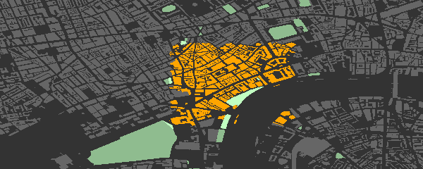 Note the `border = 0` argument on the last call divides the park
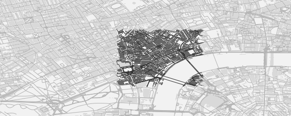
polygons precisely along the border. The same map highlighted in
dark-on-light:
``` r
map <- osm_basemap (bbox = bbox, bg = "gray95")
map <- add_osm_groups (map, dat_B, groups = pts, cols = "gray40", bg = "gray85")
map <- add_osm_groups (map, dat_H, groups = pts, cols = "gray20", bg = "gray70")
print_osm_map (map)
```
Note the `border = 0` argument on the last call divides the park
polygons precisely along the border. The same map highlighted in
dark-on-light:
``` r
map <- osm_basemap (bbox = bbox, bg = "gray95")
map <- add_osm_groups (map, dat_B, groups = pts, cols = "gray40", bg = "gray85")
map <- add_osm_groups (map, dat_H, groups = pts, cols = "gray20", bg = "gray70")
print_osm_map (map)
```
 ------------------------------------------------------------------------
## 5. Highlighting Clusters
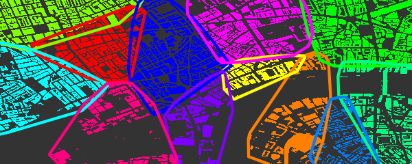
`add_osm_groups` also enables plotting an entire region as a group of
spatially distinct clusters of defined colours. Groups can be defined by
simple spatial points denoting their centres:
``` r
set.seed (2)
ngroups <- 12
x <- bbox [1, 1] + runif (ngroups) * diff (bbox [1, ])
y <- bbox [2, 1] + runif (ngroups) * diff (bbox [2, ])
groups <- as.list (data.frame (t (cbind (x, y))))
```
Calling `add_osm_groups` with no `bg` argument forces all points lying
outside those defined groups to be allocated to the nearest groups, and
thus produces an inclusive grouping extending across an entire region.
``` r
map <- osm_basemap (bbox = bbox, bg = "gray20")
map <- add_osm_groups (
map,
dat_B,
groups = groups,
cols = rainbow (length (groups)),
border_width = 2
)
print_osm_map (map)
```
------------------------------------------------------------------------
## 5. Highlighting Clusters
`add_osm_groups` also enables plotting an entire region as a group of
spatially distinct clusters of defined colours. Groups can be defined by
simple spatial points denoting their centres:
``` r
set.seed (2)
ngroups <- 12
x <- bbox [1, 1] + runif (ngroups) * diff (bbox [1, ])
y <- bbox [2, 1] + runif (ngroups) * diff (bbox [2, ])
groups <- as.list (data.frame (t (cbind (x, y))))
```
Calling `add_osm_groups` with no `bg` argument forces all points lying
outside those defined groups to be allocated to the nearest groups, and
thus produces an inclusive grouping extending across an entire region.
``` r
map <- osm_basemap (bbox = bbox, bg = "gray20")
map <- add_osm_groups (
map,
dat_B,
groups = groups,
cols = rainbow (length (groups)),
border_width = 2
)
print_osm_map (map)
```
 ------------------------------------------------------------------------
## 6. Highlighting Areas Bounded by Named Highways
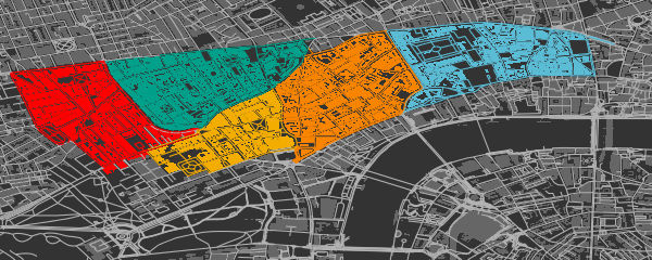
An alternative way of defining highlighted groups is by naming the
highways encircling desired regions.
``` r
# These highways extend beyond the previous, smaller bbox
bbox_big <- get_bbox (c (-0.15, 51.5, -0.10, 51.52))
highways <- c (
"Davies.St", "Berkeley.Sq", "Berkeley.St", "Piccadilly",
"Regent.St", "Oxford.St"
)
highways1 <- connect_highways (highways = highways, bbox = bbox_big)
highways <- c ("Regent.St", "Oxford.St", "Shaftesbury")
highways2 <- connect_highways (highways = highways, bbox = bbox_big)
highways <- c (
"Piccadilly", "Shaftesbury.Ave", "Charing.Cross.R",
"Saint.Martin", "Trafalgar.Sq", "Cockspur.St",
"Pall.Mall", "St.James"
)
highways3 <- connect_highways (highways = highways, bbox = bbox_big)
highways <- c (
"Charing.Cross", "Duncannon.St", "Strand", "Aldwych",
"Kingsway", "High.Holborn", "Shaftesbury.Ave"
)
highways4 <- connect_highways (highways = highways, bbox = bbox_big)
highways <- c (
"Kingsway", "Holborn", "Farringdon.St", "Strand",
"Fleet.St", "Aldwych"
)
highways5 <- connect_highways (highways = highways, bbox = bbox_big)
groups <- list (highways1, highways2, highways3, highways4, highways5)
```
And then passing these lists of groups returned by `connect_highways` to
`add_osm_groups`, this time with some Wes Anderson flair.
``` r
map <- osm_basemap (bbox = bbox, bg = "gray20")
library (wesanderson)
cols <- wes_palette ("Darjeeling", 5)
map <- add_osm_groups (
map,
dat_B,
groups = groups,
boundary = 1,
cols = cols,
bg = "gray40",
colmat = FALSE
)
map <- add_osm_groups (
map,
dat_H,
groups = groups,
boundary = 0,
cols = cols,
bg = "gray70",
colmat = FALSE
)
print_osm_map (map)
```
------------------------------------------------------------------------
## 6. Highlighting Areas Bounded by Named Highways
An alternative way of defining highlighted groups is by naming the
highways encircling desired regions.
``` r
# These highways extend beyond the previous, smaller bbox
bbox_big <- get_bbox (c (-0.15, 51.5, -0.10, 51.52))
highways <- c (
"Davies.St", "Berkeley.Sq", "Berkeley.St", "Piccadilly",
"Regent.St", "Oxford.St"
)
highways1 <- connect_highways (highways = highways, bbox = bbox_big)
highways <- c ("Regent.St", "Oxford.St", "Shaftesbury")
highways2 <- connect_highways (highways = highways, bbox = bbox_big)
highways <- c (
"Piccadilly", "Shaftesbury.Ave", "Charing.Cross.R",
"Saint.Martin", "Trafalgar.Sq", "Cockspur.St",
"Pall.Mall", "St.James"
)
highways3 <- connect_highways (highways = highways, bbox = bbox_big)
highways <- c (
"Charing.Cross", "Duncannon.St", "Strand", "Aldwych",
"Kingsway", "High.Holborn", "Shaftesbury.Ave"
)
highways4 <- connect_highways (highways = highways, bbox = bbox_big)
highways <- c (
"Kingsway", "Holborn", "Farringdon.St", "Strand",
"Fleet.St", "Aldwych"
)
highways5 <- connect_highways (highways = highways, bbox = bbox_big)
groups <- list (highways1, highways2, highways3, highways4, highways5)
```
And then passing these lists of groups returned by `connect_highways` to
`add_osm_groups`, this time with some Wes Anderson flair.
``` r
map <- osm_basemap (bbox = bbox, bg = "gray20")
library (wesanderson)
cols <- wes_palette ("Darjeeling", 5)
map <- add_osm_groups (
map,
dat_B,
groups = groups,
boundary = 1,
cols = cols,
bg = "gray40",
colmat = FALSE
)
map <- add_osm_groups (
map,
dat_H,
groups = groups,
boundary = 0,
cols = cols,
bg = "gray70",
colmat = FALSE
)
print_osm_map (map)
```
 ------------------------------------------------------------------------
## 7. Data Surfaces
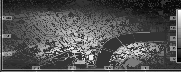
Finally, `osmplotr` contains a function `add_osm_surface` that spatially
interpolates a given set of spatial data points and colours OSM objects
according to a specified colour gradient. This is illustrated here with
the `volcano` data projected onto the `bbox`.
``` r
x <- seq (bbox [1, 1], bbox [1, 2], length.out = dim (volcano) [1])
y <- seq (bbox [2, 1], bbox [2, 2], length.out = dim (volcano) [2])
xy <- cbind (rep (x, dim (volcano) [2]), rep (y, each = dim (volcano) [1]))
z <- as.numeric (volcano)
dat <- data.frame (x = xy [, 1], y = xy [, 2], z = z)
```
``` r
map <- osm_basemap (bbox = bbox, bg = "gray20")
cols <- gray (0:50 / 50)
map <- add_osm_surface (map, dat_B, dat = dat, cols = cols)
# Darken cols by ~20%
map <- add_osm_surface (
map,
dat_H,
dat = dat,
cols = adjust_colours (cols, -0.2)
)
map <- add_colourbar (map, cols = cols, zlims = range (volcano))
map <- add_axes (map)
print_osm_map (map)
```
------------------------------------------------------------------------
## 7. Data Surfaces
Finally, `osmplotr` contains a function `add_osm_surface` that spatially
interpolates a given set of spatial data points and colours OSM objects
according to a specified colour gradient. This is illustrated here with
the `volcano` data projected onto the `bbox`.
``` r
x <- seq (bbox [1, 1], bbox [1, 2], length.out = dim (volcano) [1])
y <- seq (bbox [2, 1], bbox [2, 2], length.out = dim (volcano) [2])
xy <- cbind (rep (x, dim (volcano) [2]), rep (y, each = dim (volcano) [1]))
z <- as.numeric (volcano)
dat <- data.frame (x = xy [, 1], y = xy [, 2], z = z)
```
``` r
map <- osm_basemap (bbox = bbox, bg = "gray20")
cols <- gray (0:50 / 50)
map <- add_osm_surface (map, dat_B, dat = dat, cols = cols)
# Darken cols by ~20%
map <- add_osm_surface (
map,
dat_H,
dat = dat,
cols = adjust_colours (cols, -0.2)
)
map <- add_colourbar (map, cols = cols, zlims = range (volcano))
map <- add_axes (map)
print_osm_map (map)
```
 ------------------------------------------------------------------------
## 8. Gallery
Got a nice `osmplotr` map? Please contribute in one of the following
ways:
1. Fork repo, add link to `README.md/.Rmd`, and send pull request; or
2. Open issue with details; or
3. Send email to address in
[`DESCRIPTION`](https://github.com/ropensci/osmplotr/blob/master/DESCRIPTION).
------------------------------------------------------------------------
See package vignettes ([basic
maps](https://docs.ropensci.org/osmplotr/articles/basic-maps.html) and
[data maps](https://docs.ropensci.org/osmplotr/articles/data-maps.html))
for a lot more detail and further capabilities of `osmplotr`. Please
note that this project is released with a [Contributor Code of
Conduct](https://ropensci.org/code-of-conduct/). By participating in
this project you agree to abide by its terms.
------------------------------------------------------------------------
[](https://ropensci.org/)
------------------------------------------------------------------------
## 8. Gallery
Got a nice `osmplotr` map? Please contribute in one of the following
ways:
1. Fork repo, add link to `README.md/.Rmd`, and send pull request; or
2. Open issue with details; or
3. Send email to address in
[`DESCRIPTION`](https://github.com/ropensci/osmplotr/blob/master/DESCRIPTION).
------------------------------------------------------------------------
See package vignettes ([basic
maps](https://docs.ropensci.org/osmplotr/articles/basic-maps.html) and
[data maps](https://docs.ropensci.org/osmplotr/articles/data-maps.html))
for a lot more detail and further capabilities of `osmplotr`. Please
note that this project is released with a [Contributor Code of
Conduct](https://ropensci.org/code-of-conduct/). By participating in
this project you agree to abide by its terms.
------------------------------------------------------------------------
[](https://ropensci.org/)