{
"cells": [
{
"cell_type": "markdown",
"metadata": {
"slideshow": {
"slide_type": "slide"
}
},
"source": [
"# Stochastic Processes:
Data Analysis and Computer Simulation\n",
"
\n",
"\n",
"\n",
"# Python programming for beginners\n",
"
\n",
"\n",
"# 4. Simulating a damped harmonic oscillator\n",
"
"
]
},
{
"cell_type": "markdown",
"metadata": {
"slideshow": {
"slide_type": "slide"
}
},
"source": [
"# 4.1. A damped harmonic oscillator"
]
},
{
"cell_type": "markdown",
"metadata": {
"slideshow": {
"slide_type": "-"
}
},
"source": [
"## Model system\n",
"\n",
"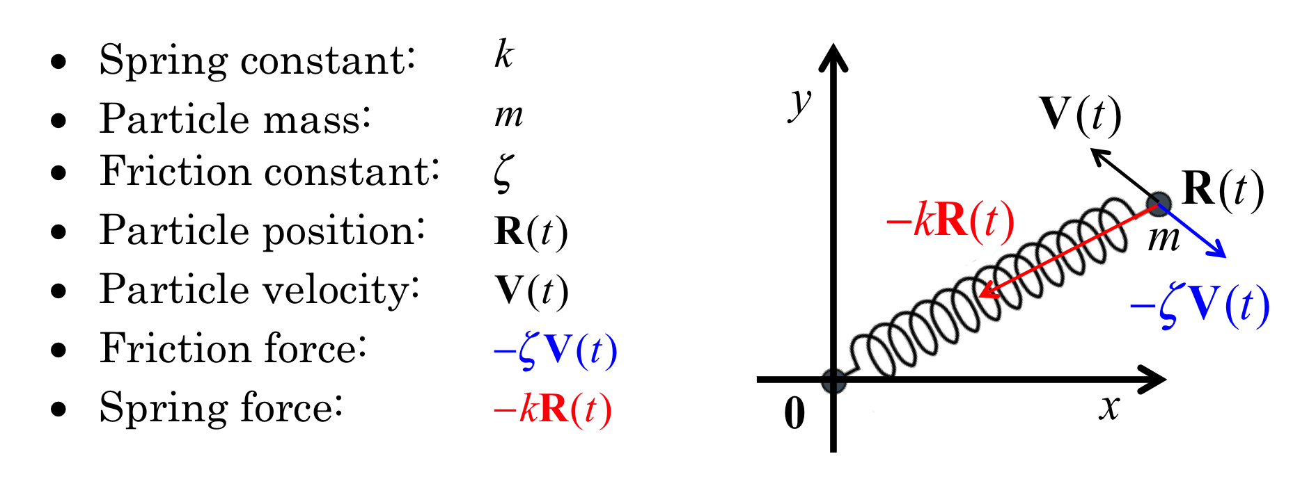 "
]
},
{
"cell_type": "markdown",
"metadata": {
"slideshow": {
"slide_type": "slide"
}
},
"source": [
"## Time evolution equations\n",
"\n",
"$$\n",
"\\frac{d\\mathbf{R}(t)}{dt} =\\mathbf{V}(t)\\hspace{17mm} \\tag{B1}\n",
"$$\n",
"\n",
"$$\n",
"m\\frac{d\\mathbf{V}(t)}{dt}=-\\zeta\\mathbf{V}(t)-k\\mathbf{R}(t) \\tag{B2}\n",
"$$"
]
},
{
"cell_type": "markdown",
"metadata": {
"slideshow": {
"slide_type": "slide"
}
},
"source": [
"# 4.2. Computer simulation"
]
},
{
"cell_type": "markdown",
"metadata": {},
"source": [
"## Euler method\n",
"\n",
"- Use Eq.(A8) in the previous lessen\n",
"\n",
"$$\n",
"\\mathbf{R}_{i+1}=\\mathbf{R}_i+\\int_{t_i}^{t_{i+1}} dt\\mathbf{V}(t)\\simeq\\mathbf{R}_i+\\mathbf{V}_i \\Delta t \\hspace{15mm}\\tag{B3}\n",
"$$\n",
"\n",
"$$\n",
"\\mathbf{V}_{i+1}=\\mathbf{V}_i-\\frac{\\zeta}{m}\\int_{t_i}^{t_{i+1}} dt\\mathbf{V}(t)-\\frac{k}{m}\\int_{t_i}^{t_{i+1}} dt\\mathbf{R}(t)\n",
"$$\n",
"$$\n",
"\\simeq\\left(1-\\frac{\\zeta}{m}\\Delta t\\right)\\mathbf{V}_i - \\frac{k}{m} \\mathbf{R}_i \\Delta t \\hspace{12mm}\\tag{B4}\n",
"$$"
]
},
{
"cell_type": "markdown",
"metadata": {
"slideshow": {
"slide_type": "slide"
}
},
"source": [
"## Import libraries"
]
},
{
"cell_type": "code",
"execution_count": null,
"metadata": {
"scrolled": true,
"slideshow": {
"slide_type": "-"
}
},
"outputs": [],
"source": [
"%matplotlib inline\n",
"import numpy as np\n",
"import matplotlib.pyplot as plt\n",
"import matplotlib.animation as animation\n",
"from IPython.display import HTML\n",
"plt.style.use('ggplot')"
]
},
{
"cell_type": "markdown",
"metadata": {
"slideshow": {
"slide_type": "slide"
}
},
"source": [
"## Define variables"
]
},
{
"cell_type": "code",
"execution_count": null,
"metadata": {
"scrolled": true,
"slideshow": {
"slide_type": "-"
}
},
"outputs": [],
"source": [
"dim = 2 # system dimension (x,y)\n",
"nums = 1000 # number of steps\n",
"R = np.zeros(dim) # particle position\n",
"V = np.zeros(dim) # particle velocity\n",
"Rs = np.zeros([dim,nums]) # particle position (at all steps)\n",
"Vs = np.zeros([dim,nums]) # particle velocity (at all steps)\n",
"Et = np.zeros(nums) # total enegy of the system (at all steps)\n",
"time = np.zeros(nums) # time (at all steps)"
]
},
{
"cell_type": "markdown",
"metadata": {
"slideshow": {
"slide_type": "slide"
}
},
"source": [
"## Define functions"
]
},
{
"cell_type": "code",
"execution_count": null,
"metadata": {},
"outputs": [],
"source": [
"def init(): # initialize animation\n",
" particles.set_data([], [])\n",
" line.set_data([], [])\n",
" title.set_text(r'')\n",
" return particles,line,title\n",
"def animate(i): # define amination using Euler\n",
" global R,V,F,Rs,Vs,time,Et\n",
" R, V = R+V*dt, V*(1-zeta/m*dt)-k/m*dt*R # Euler method Eqs.(B3)&(B4)\n",
" Rs[0:dim,i]=R\n",
" Vs[0:dim,i]=V\n",
" time[i]=i*dt\n",
" Et[i]=0.5*m*np.linalg.norm(V)**2+0.5*k*np.linalg.norm(R)**2\n",
" particles.set_data(R[0], R[1]) # current position\n",
" line.set_data(Rs[0,0:i], Rs[1,0:i]) # add latest position Rs\n",
" title.set_text(r\"$t = {0:.2f},E_T = {1:.3f}$\".format(i*dt,Et[i]))\n",
" return particles,line,title"
]
},
{
"cell_type": "markdown",
"metadata": {
"slideshow": {
"slide_type": "slide"
}
},
"source": [
"## Perform the simulation"
]
},
{
"cell_type": "code",
"execution_count": null,
"metadata": {},
"outputs": [],
"source": [
"# System parameters\n",
"# particle mass, spring & friction constants\n",
"m, k, zeta = 1.0, 1.0, 0.25\n",
"# Initial condition\n",
"R[0], R[1] = 1., 1. # Rx(0), Ry(0)\n",
"V[0], V[1] = 1., 0. # Vx(0), Vy(0)\n",
"dt = 0.1*np.sqrt(k/m) # set \\Delta t\n",
"box = 5 # set size of draw area\n",
"# set up the figure, axis, and plot element for animatation\n",
"fig, ax = plt.subplots(figsize=(7.5,7.5)) # setup plot\n",
"ax = plt.axes(xlim=(-box/2,box/2),ylim=(-box/2,box/2)) # draw range\n",
"particles, = ax.plot([],[],'ko', ms=10) # setup plot for particle \n",
"line,=ax.plot([],[],lw=1) # setup plot for trajectry\n",
"title=ax.text(0.5,1.05,r'',transform=ax.transAxes,va='center') # title\n",
"anim=animation.FuncAnimation(fig,animate,init_func=init,\n",
" frames=nums,interval=5,blit=True,repeat=False) # draw animation\n",
"# anim.save('movie.mp4',fps=20,dpi=400)\n",
"# \"conda install ffmpeg\"\n",
"HTML(anim.to_html5_video()) "
]
},
{
"cell_type": "markdown",
"metadata": {
"slideshow": {
"slide_type": "slide"
}
},
"source": [
"## Analyze the simulation results "
]
},
{
"cell_type": "markdown",
"metadata": {},
"source": [
"### Temporal values of $R_x(t)$, $R_y(t)$, $E_T(t)$ \n",
"\n",
"- Total energy of the harmonic oscillator\n",
"$$\n",
"E_T(t)=E_{kinetic}(t) + E_{potential}(t) = \\frac{1}{2}m\\mathbf{V}^2(t)+\\frac{1}{2}k\\mathbf{R}^2(t)\n",
"$$"
]
},
{
"cell_type": "code",
"execution_count": null,
"metadata": {
"scrolled": false,
"slideshow": {
"slide_type": "-"
}
},
"outputs": [],
"source": [
"fig, ax = plt.subplots(figsize=(7.5,7.5))\n",
"ax.set_xlabel(r\"$t$\", fontsize=20)\n",
"ax.plot(time,Rs[0]) # plot R_x(t)\n",
"ax.plot(time,Rs[1]) # plot R_y(t)\n",
"ax.plot(time,Et) # plot E(t) (ideally constant if \\deta=0)\n",
"ax.legend([r'$R_x(t)$',r'$R_y(t)$',r'$E_T(t)$'], fontsize=14)\n",
"plt.show()"
]
},
{
"cell_type": "markdown",
"metadata": {
"slideshow": {
"slide_type": "slide"
}
},
"source": [
"### Trajectory plot"
]
},
{
"cell_type": "code",
"execution_count": null,
"metadata": {
"scrolled": false,
"slideshow": {
"slide_type": "-"
}
},
"outputs": [],
"source": [
"fig, ax = plt.subplots(figsize=(7.5,7.5))\n",
"ax.plot(Rs[0,0:nums],Rs[1,0:nums]) # parameteric plot Rx(t) vs. Ry(t)\n",
"plt.show()"
]
},
{
"cell_type": "markdown",
"metadata": {
"slideshow": {
"slide_type": "slide"
}
},
"source": [
"# Supplemental Note: Simulation schemes with other methods\n",
"\n",
"- The original Euler method is not correctly applicable to the oscillator problem unless the friction constant is sufficiently large. In general, oscillator problems have to be solved with higher order methods such as the Runge-Kutta or the Leap-Frog shown below.\n",
"\n",
"## Runge-Kutta 2nd order method\n",
"\n",
"- Use Eqs.(A15) and (A16) in the previous lessen\n",
"\n",
"$$\n",
"\\mathbf{R}'_{i+\\frac{1}{2}}=\n",
"\\mathbf{R}_i+\\frac{\\Delta t}{2}\\mathbf{V}_{i} \\hspace{15mm}\\tag{B5}\n",
"$$\n",
"\n",
"$$\n",
"\\mathbf{V}'_{i+\\frac{1}{2}}=\n",
"\\mathbf{V}_i-\\frac{\\zeta}{m}\\frac{\\Delta t}{2}\\mathbf{V}_{i} - \\frac{k}{m} \\frac{\\Delta t}{2}\\mathbf{R}_{i} \\hspace{12mm}\\tag{B6}\n",
"$$\n",
"\n",
"$$\n",
"\\mathbf{R}_{i+1}=\n",
"\\mathbf{R}_i+\\Delta t\\mathbf{V}'_{i+\\frac{1}{2}} \\hspace{15mm}\\tag{B7}\n",
"$$\n",
"\n",
"$$\n",
"\\mathbf{V}_{i+1}=\n",
"\\mathbf{V}_i-\\frac{\\zeta}{m}\\Delta t\\mathbf{V}'_{i+\\frac{1}{2}} - \\frac{k}{m} \\Delta t\\mathbf{R}'_{i+\\frac{1}{2}} \\hspace{12mm}\\tag{B8}\n",
"$$\n"
]
},
{
"cell_type": "markdown",
"metadata": {
"slideshow": {
"slide_type": "slide"
}
},
"source": [
"## Runge-Kutta 4th order method\n",
"- Use Eqs.(A18) - (A21) in the previous lessen\n",
"$$\n",
"\\mathbf{R}'_{i+\\frac{1}{2}}=\n",
"\\mathbf{R}_i+\\frac{\\Delta t}{2}\\mathbf{V}_{i} \\hspace{15mm}\\tag{B9}\n",
"$$\n",
"$$\n",
"\\mathbf{V}'_{i+\\frac{1}{2}}=\n",
"\\mathbf{V}_i-\\frac{\\zeta}{m}\\frac{\\Delta t}{2}\\mathbf{V}_{i} - \\frac{k}{m} \\frac{\\Delta t}{2}\\mathbf{R}_{i} \\hspace{12mm}\\tag{B10}\n",
"$$\n",
"$$\n",
"\\mathbf{R}''_{i+\\frac{1}{2}}=\n",
"\\mathbf{R}_i+\\frac{\\Delta t}{2}\\mathbf{V}'_{i+\\frac{1}{2}} \\hspace{15mm}\\tag{B11}\n",
"$$\n",
"$$\n",
"\\mathbf{V}''_{i+\\frac{1}{2}}=\n",
"\\mathbf{V}_i-\\frac{\\zeta}{m}\\frac{\\Delta t}{2}\\mathbf{V}'_{i+\\frac{1}{2}} - \\frac{k}{m} \\frac{\\Delta t}{2}\\mathbf{R}'_{i+\\frac{1}{2}} \\hspace{12mm}\\tag{B12}\n",
"$$\n",
"$$\n",
"\\mathbf{R}'''_{i+1}=\n",
"\\mathbf{R}_i+{\\Delta t}\\mathbf{V}''_{i+\\frac{1}{2}} \\hspace{15mm}\\tag{B13}\n",
"$$\n",
"$$\n",
"\\mathbf{V}'''_{i+1}=\n",
"\\mathbf{V}_i-\\frac{\\zeta}{m}\\Delta t\\mathbf{V}''_{i+\\frac{1}{2}} - \\frac{k}{m} \\Delta t\\mathbf{R}''_{i+\\frac{1}{2}} \\hspace{12mm}\\tag{B14}\n",
"$$\n",
"$$\n",
"\\mathbf{R}_{i+1}=\n",
"\\mathbf{R}_i+\\frac{\\Delta t}{6}\\left(\\mathbf{V}_{i}+2\\mathbf{V}'_{i+\\frac{1}{2}}+2\\mathbf{V}''_{i+\\frac{1}{2}}+\\mathbf{V}'''_{i+1}\\right) \\hspace{15mm}\\tag{B15}\n",
"$$\n",
"$$\n",
"\\mathbf{V}_{i+1}=\n",
"\\mathbf{V}_i-\\frac{\\zeta}{m}\\frac{\\Delta t}{6}\\left(\\mathbf{V}_{i}+2\\mathbf{V}'_{i+\\frac{1}{2}}+2\\mathbf{V}''_{i+\\frac{1}{2}}+\\mathbf{V}'''_{i+1}\\right) \n",
"$$\n",
"$$\n",
"\\hspace{15mm}- \\frac{k}{m} \\frac{\\Delta}{6} t\\left(\\mathbf{R}_{i}+2\\mathbf{R}'_{i+\\frac{1}{2}}+2\\mathbf{R}''_{i+\\frac{1}{2}}+\\mathbf{R}'''_{i+1}\\right) \\hspace{12mm}\\tag{B16}\n",
"$$"
]
},
{
"cell_type": "markdown",
"metadata": {
"slideshow": {
"slide_type": "slide"
}
},
"source": [
"## Leap-Frog method\n",
"- Use Eqs.(A11) - (A14) in the previous lessen\n",
"$$\n",
"\\mathbf{V}_{i,n+\\frac{1}{2}}\n",
"=\\mathbf{V}_{i,n-\\frac{1}{2}}-\\frac{\\zeta}{m}\\Delta t\\mathbf{V}_{i,n} \n",
"- \\frac{k}{m}\\mathbf{R}_{i,n}\\Delta t \\\\\n",
"\\hspace{30mm}=\\mathbf{V}_{i,n-\\frac{1}{2}}\n",
"-\\frac{\\zeta}{m}\\Delta t\\frac{1}{2}\\left(\n",
"\\mathbf{V}_{i,n+\\frac{1}{2}}+\\mathbf{V}_{i,n-\\frac{1}{2}}\n",
"\\right) \\\\\n",
"- \\frac{k}{m}\\mathbf{R}_{i,n}\\Delta t\n",
"$$\n",
"\n",
"$$\n",
"\\therefore\\ \\ \\ \\mathbf{V}_{i,n+\\frac{1}{2}}\n",
"=\\left(\\left(1-\\frac{\\zeta}{2m}\\Delta t\\right)\\mathbf{V}_{i,n-\\frac{1}{2}}\n",
"- \\frac{k}{m}\\mathbf{R}_{i,n}\\Delta t \\right)\\\\\n",
"\\times\\left(1+\\frac{\\zeta}{2m}\\Delta t\\right)^{-1}\n",
"\\tag{B17}\n",
"$$\n",
"\n",
"\n",
"$$\n",
"\\mathbf{R}_{i,n+1}=\\mathbf{R}_{i,n}+\\mathbf{V}_{i,n+\\frac{1}{2}}\\Delta t \\hspace{15mm}\\tag{B18}\n",
"$$\n",
"\n",
"- The following equation is needed only when you need to know $\\mathbf{R}_{i,n+\\frac{1}{2}}$, for example to calculate the temporal total energy $E(t)$ at $t_{n+\\frac{1}{2}}$.\n",
"\n",
"$$\n",
"\\mathbf{R}_{i,n+\\frac{1}{2}}\n",
"=\\frac{1}{2}\\left(\\mathbf{R}_{i,n+1}+\\mathbf{R}_{i,n}\\right)\n",
"\\tag{B19}\n",
"$$\n"
]
},
{
"cell_type": "code",
"execution_count": null,
"metadata": {},
"outputs": [],
"source": []
}
],
"metadata": {
"anaconda-cloud": {},
"celltoolbar": "Slideshow",
"kernelspec": {
"display_name": "Python 3 (ipykernel)",
"language": "python",
"name": "python3"
},
"language_info": {
"codemirror_mode": {
"name": "ipython",
"version": 3
},
"file_extension": ".py",
"mimetype": "text/x-python",
"name": "python",
"nbconvert_exporter": "python",
"pygments_lexer": "ipython3",
"version": "3.9.13"
}
},
"nbformat": 4,
"nbformat_minor": 2
}