__CTF Solution__
__Some approximate solutions__
Most of the challengers viewed logreg solvers (e.g. scikit logreg) as a blackbox oracle, and used some stochastic approach to guess the missing dataset row, trying to optimize the distance between _‖ 𝚕𝚘𝚐𝚛𝚎𝚐(guessed dataset) − provided model ‖_
After trying multiple small modifications and iterating, they ended up with a solution vector, that gave a model within $10^{−5}$ of the provided one.
xn=[3,14,4,-3,-13,11,-5,-16,16,16,-12, 0,9,1,-11-14]
yn=0
But then, how to verify that this empirical result was really the golden solution? Enumerating the space of $32^{16}$ possibilities would be far too slow? Also, the distance ≤ 0.5 ⋅ $10^{−5}$ was small, but not zero: would there be a thin chance, that there exist another logreg solver, that would yield a closer solution?
I bet some of the challengers got a real headache about all these thoughts?
Some may have even thought that the whole problem was ill-defined! Or that the only way of verifying the solution was to ask the CTF organizers :)
It is now time to straighten out the whole story!
__The real solution__

```python
# Load trained model from csv
trained_model_data = pd.read_csv("trained_LR_model.csv", index_col=False)
theta_best_bar = trained_model_data[[f"theta_{i}" for i in range(k+1)]].to_numpy().reshape(-1)
print("theta_best_bar: %s" % theta_best_bar)
# Load attacker knowledge of N-1 points
df = pd.read_csv("attacker_knowledge.csv", index_col=False)
X = df[[f"V{i}" for i in range(1, k+1)]].to_numpy()
y = df["target"].to_numpy()
print("dimensions of X: %s x %s" % X.shape)
print("dimension of y: %s" % y.shape)
# Helper functions
sigmoid = lambda z: 1/(1+np.exp(-z))
# gradient of logreg over the (partial) dataset X,y at theta_bar
def gradient_log_reg(X, y, theta_bar):
"""Gradient of the logistic regression loss function (regularization=1).
Args:
X: Features.
y: Labels.
theta_bar: weights (with intercept coeff prepended).
Returns:
Computed gradient evaluated at given values.
"""
theta = theta_bar[1:]
X_bar = np.hstack((np.ones((len(X),1)), X))
y_hat = sigmoid(X_bar@theta_bar)
return (y_hat-y)@X_bar + np.hstack(([0], theta))
# the known vector of the awesome equality of the CTF
# is the opposite of the partial gradient
known_vector = -gradient_log_reg(X, y, theta_best_bar)
print('This is the known vector: %s' % known_vector)
```
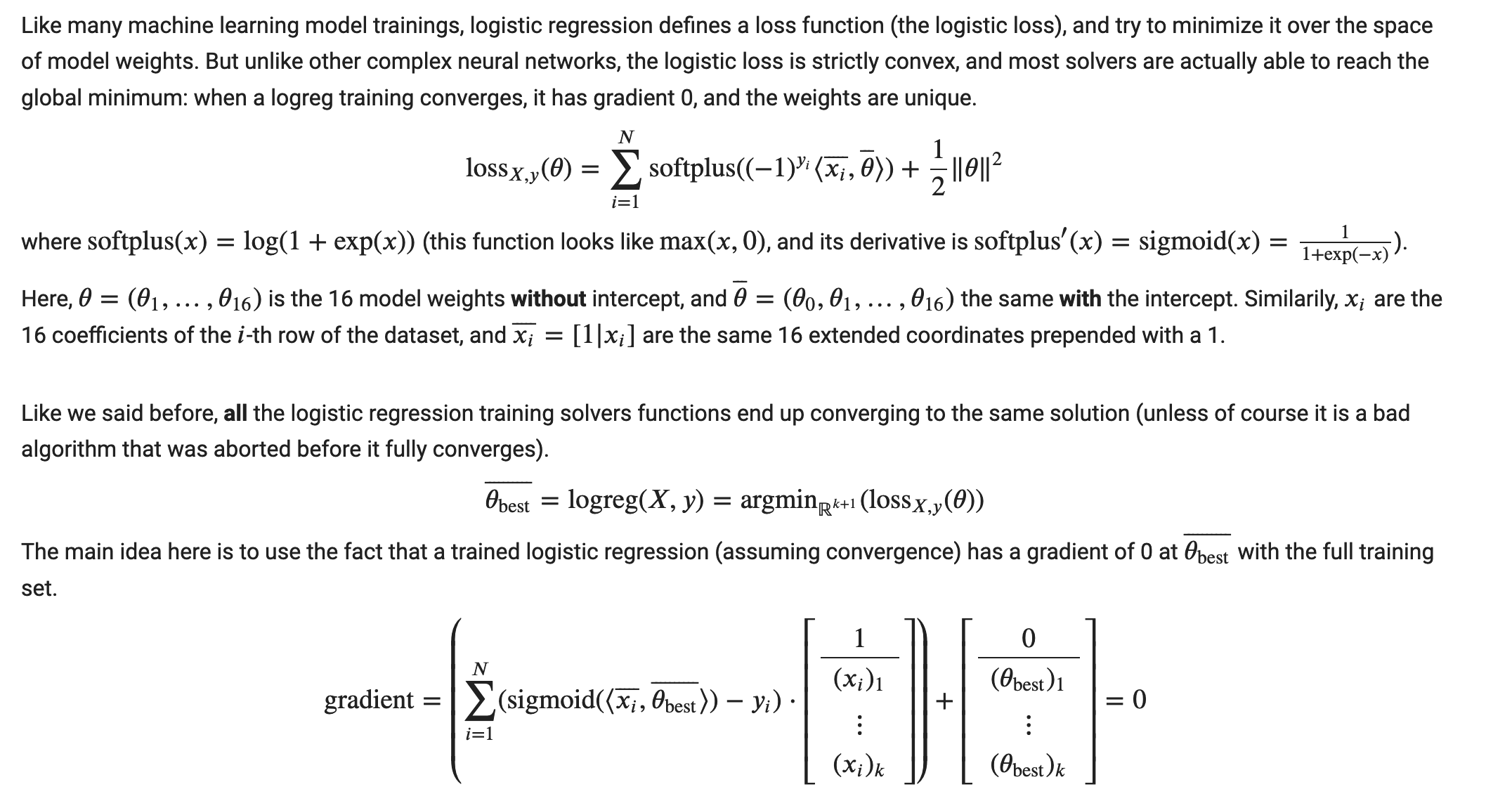
Let's recall the awesome equality (in red the unknowns, on the right what we just computed):
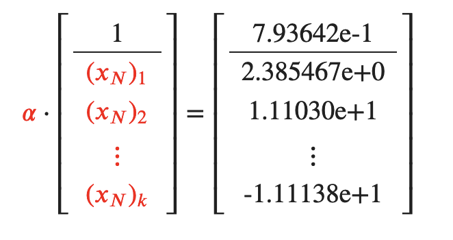
The first coordinate reveals the value of 𝛼, and the other 16 coordinates (divided by 𝛼) reveal the missing datapoint 𝑥𝑁!
```Python
alpha = known_vector[0]
recovered_xn = [known_vector[i+1]/alpha for i in range(k)]
print("alpha: %s" % alpha)
print("recovered x_500: %s" % recovered_xn)
```
```Python
final_xn = np.round(recovered_xn)
print("final_xn: %s" % final_xn)
```
final_xn: [ 3. 14. 4. -3. -13. 11. -5. -16. 16. 16. -12. 0. 9. 1. -11. -14.]
We can now safely rest assured that there is no other solution in the whole search space!
Finally, since 𝛼 in the awesome equality is equal to sigmoid(something) − 𝑦𝑁, and sigmoid yields values in the open real interval (0,1), we deduce that 𝛼 is positive if 𝑦𝑁 is 0, and negative otherwise if 𝑦𝑁 is 1.
So the sign of 𝛼 discloses the class of the missing sample.
```Python
final_yn = 1 if alpha<0 else 0
print("final yn: %s" % final_yn)
```
And this concludes this CTF exercice!
On a side note, you also understand why it was important to provide 𝜃 with at least 5 decimal digits of precision.
If we had decided to add some differential privacy noise (say 2% of noise to the coordinates of theta), the same problem would now have a ton of potential solutions (because the error per coordinate would be much larger than 16, instead of < 0.5).
In other words, adding just a little amount of differential privacy noise would have made this reconstruction attack fail, a general principle that is good to keep in mind!