{
"cells": [
{
"cell_type": "markdown",
"metadata": {},
"source": [
"# matplotlib\n",
"\n",
"Matplotlib is the core plotting package in scientific python. There are others to explore as well (which we'll chat about on slack).\n",
"\n",
"Note: the latest version of matplotlib (2.0) introduced a number of style changes. This is the version we use here.\n",
"\n",
"Also, there are different interfaces for interacting with matplotlib, an interactive, function-driven (state machine) commandset and an object-oriented version. Usually for interactive work, we use the state interface."
]
},
{
"cell_type": "markdown",
"metadata": {},
"source": [
"We want matplotlib to work inline in the notebook."
]
},
{
"cell_type": "code",
"execution_count": null,
"metadata": {
"collapsed": true
},
"outputs": [],
"source": [
"%matplotlib inline"
]
},
{
"cell_type": "code",
"execution_count": null,
"metadata": {
"collapsed": true
},
"outputs": [],
"source": [
"import numpy as np\n",
"import matplotlib.pyplot as plt"
]
},
{
"cell_type": "markdown",
"metadata": {},
"source": [
"## Matplotlib concepts\n",
"\n",
"Matplotlib was designed with the following goals (from mpl docs):\n",
"\n",
"* Plots should look great -- publication quality (e.g. antialiased)\n",
"* Postscript output for inclusion with TeX documents\n",
"* Embeddable in a graphical user interface for application development\n",
"* Code should be easy to understand it and extend\n",
"* Making plots should be easy\n",
"\n",
"Matplotlib is mostly for 2-d data, but there are some basic 3-d (surface) interfaces.\n",
"\n",
"Volumetric data requires a different approach"
]
},
{
"cell_type": "markdown",
"metadata": {},
"source": [
"### Gallery\n",
"\n",
"Matplotlib has a great gallery on their webpage -- find something there close to what you are trying to do and use it as a starting point:\n",
"\n",
"http://matplotlib.org/gallery.html"
]
},
{
"cell_type": "markdown",
"metadata": {},
"source": [
"### Importing\n",
"\n",
"There are several different interfaces for matplotlib (see http://matplotlib.org/faq/usage_faq.html)\n",
"\n",
"Basic ideas:\n",
"\n",
"* `matplotlib` is the entire package\n",
"* `matplotlib.pyplot` is a module within matplotlib that provides easy access to the core plotting routines\n",
"* `pylab` combines pyplot and numpy into a single namespace to give a MatLab like interface. You should avoid this—it might be removed in the future.\n",
"\n",
"There are a number of modules that extend its behavior, e.g. `basemap` for plotting on a sphere, `mplot3d` for 3-d surfaces\n"
]
},
{
"cell_type": "markdown",
"metadata": {},
"source": [
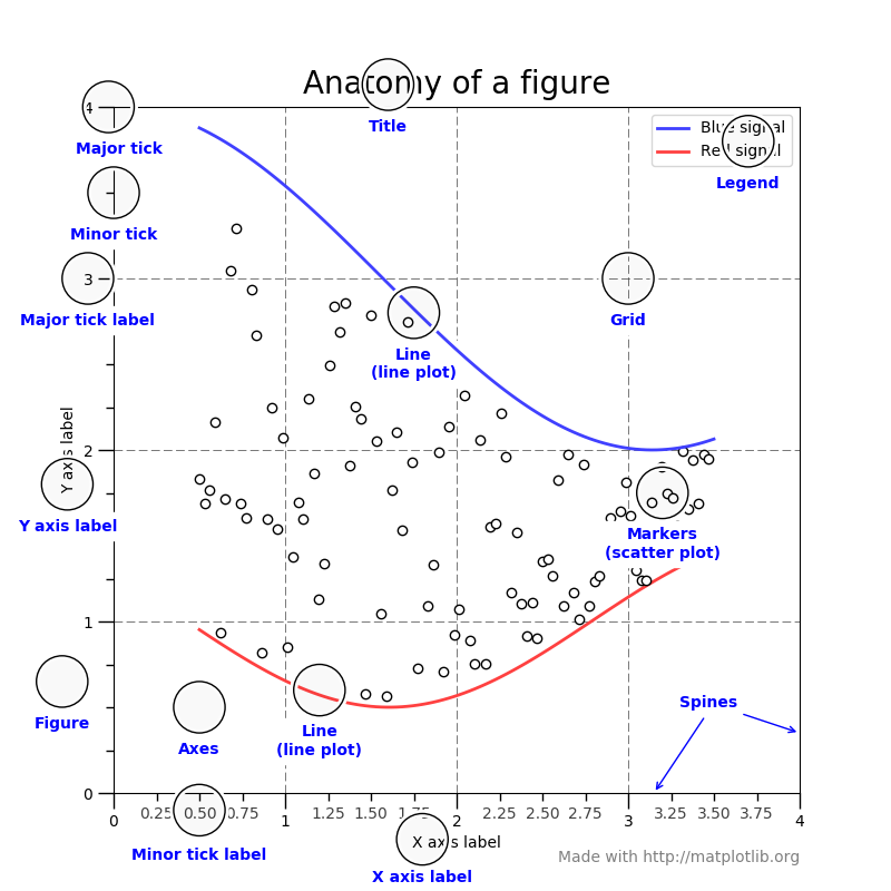
"### Anatomy of a figure\n",
"\n",
"Figures are the highest level obect and can inlcude multiple axes\n",
"\n",
"\n",
"(figure from: http://matplotlib.org/faq/usage_faq.html#parts-of-a-figure )\n"
]
},
{
"cell_type": "markdown",
"metadata": {},
"source": [
"### Backends\n",
"\n",
"Interactive backends: pygtk, wxpython, tkinter, ...\n",
"\n",
"Hardcopy backends: PNG, PDF, PS, SVG, ...\n",
"\n"
]
},
{
"cell_type": "markdown",
"metadata": {},
"source": [
"# Basic plotting"
]
},
{
"cell_type": "markdown",
"metadata": {},
"source": [
"plot() is the most basic command. Here we also see that we can use LaTeX notation for the axes"
]
},
{
"cell_type": "code",
"execution_count": null,
"metadata": {},
"outputs": [],
"source": [
"x = np.linspace(0,2.0*np.pi, num=100)\n",
"y = np.cos(x)\n",
"\n",
"plt.plot(x,y)\n",
"plt.xlabel(r\"$x$\")\n",
"plt.ylabel(r\"$\\cos(x)$\", fontsize=\"x-large\")\n",
"plt.xlim(0, 2.0*np.pi)"
]
},
{
"cell_type": "markdown",
"metadata": {},
"source": [
"Note that when we use the `plot()` command like this, matplotlib automatically creates a figure and an axis for us and it draws the plot on this for us. This is the _state machine_ interface. "
]
},
{
"cell_type": "markdown",
"metadata": {},
"source": [
" Quick Exercise:
\n",
"\n",
"We can plot 2 lines on a plot simply by calling plot twice. Make a plot with both `sin(x)` and `cos(x)` drawn\n",
"\n",
"
"
]
},
{
"cell_type": "code",
"execution_count": null,
"metadata": {
"collapsed": true
},
"outputs": [],
"source": []
},
{
"cell_type": "markdown",
"metadata": {},
"source": [
"we can use symbols instead of lines pretty easily too—and label them"
]
},
{
"cell_type": "code",
"execution_count": null,
"metadata": {},
"outputs": [],
"source": [
"plt.plot(x, np.sin(x), \"ro\", label=\"sine\")\n",
"plt.plot(x, np.cos(x), \"bx\", label=\"cosine\")\n",
"plt.xlim(0.0, 2.0*np.pi)\n",
"plt.legend(frameon=False, loc=5)"
]
},
{
"cell_type": "markdown",
"metadata": {},
"source": [
"most functions take a number of optional named argumets too"
]
},
{
"cell_type": "code",
"execution_count": null,
"metadata": {},
"outputs": [],
"source": [
"plt.plot(x, np.sin(x), \"r--\", linewidth=3.0)\n",
"plt.plot(x, np.cos(x), \"b-\")\n",
"plt.xlim(0.0, 2.0*np.pi)"
]
},
{
"cell_type": "markdown",
"metadata": {},
"source": [
"there is a command `setp()` that can also set the properties. We can get the list of settable properties as"
]
},
{
"cell_type": "code",
"execution_count": null,
"metadata": {},
"outputs": [],
"source": [
"line = plt.plot(x, np.sin(x))\n",
"plt.setp(line)"
]
},
{
"cell_type": "markdown",
"metadata": {},
"source": [
"# Multiple axes"
]
},
{
"cell_type": "markdown",
"metadata": {},
"source": [
"there are a wide range of methods for putting multiple axes on a grid. We'll look at the simplest method. All plotting commands apply to the current set of axes"
]
},
{
"cell_type": "code",
"execution_count": null,
"metadata": {},
"outputs": [],
"source": [
"plt.subplot(211)\n",
"\n",
"x = np.linspace(0,5,100)\n",
"plt.plot(x, x**3 - 4*x)\n",
"plt.xlabel(\"x\")\n",
"plt.ylabel(r\"$x^3 - 4x$\", fontsize=\"large\")\n",
"\n",
"plt.subplot(212)\n",
"\n",
"plt.plot(x, np.exp(-x**2))\n",
"plt.xlabel(\"x\")\n",
"plt.ylabel(\"Gaussian\")\n",
"\n",
"# log scale\n",
"ax = plt.gca()\n",
"ax.set_yscale(\"log\")\n",
"\n",
"# get the figure and set its size\n",
"f = plt.gcf()\n",
"f.set_size_inches(6,8)\n",
"\n",
"# tight_layout() makes sure things don't overlap\n",
"plt.tight_layout()\n",
"plt.savefig(\"test.png\")"
]
},
{
"cell_type": "markdown",
"metadata": {},
"source": [
"# Object oriented interface"
]
},
{
"cell_type": "markdown",
"metadata": {},
"source": [
"In the object oriented interface, we create a figure object, add an axis, and then interact through those objects directly."
]
},
{
"cell_type": "code",
"execution_count": null,
"metadata": {},
"outputs": [],
"source": [
"f = plt.figure()\n",
"ax = f.add_subplot(111)"
]
},
{
"cell_type": "code",
"execution_count": null,
"metadata": {},
"outputs": [],
"source": [
"x = np.linspace(0, 2*np.pi, 100)\n",
"y = np.sin(x)\n",
"ax.plot(x, y)\n",
"f"
]
},
{
"cell_type": "markdown",
"metadata": {},
"source": [
"Notice that with the state machine interface, each cell created a new figure and worked on that. Here, our `f` is a figure object, and we can refer to that figure object across multiple cells to build our figure."
]
},
{
"cell_type": "code",
"execution_count": null,
"metadata": {},
"outputs": [],
"source": [
"ax.set_xlabel(\"x\")\n",
"ax.set_ylabel(\"y\")\n",
"f"
]
},
{
"cell_type": "code",
"execution_count": null,
"metadata": {
"collapsed": true
},
"outputs": [],
"source": []
},
{
"cell_type": "markdown",
"metadata": {},
"source": [
"# Visualizing 2-d array data"
]
},
{
"cell_type": "markdown",
"metadata": {},
"source": [
"2-d datasets consist of (x, y) pairs and a value associated with that point. Here we create a 2-d Gaussian, using the `meshgrid()` function to define a rectangular set of points."
]
},
{
"cell_type": "code",
"execution_count": null,
"metadata": {
"collapsed": true
},
"outputs": [],
"source": [
"def g(x, y):\n",
" return np.exp(-((x-0.5)**2)/0.1**2 - ((y-0.5)**2)/0.2**2)\n",
"\n",
"N = 100\n",
"\n",
"x = np.linspace(0.0,1.0,N)\n",
"y = x.copy()\n",
"\n",
"xv, yv = np.meshgrid(x, y)"
]
},
{
"cell_type": "markdown",
"metadata": {},
"source": [
"A \"heatmap\" style plot assigns colors to the data values. A lot of work has gone into the latest matplotlib to define a colormap that works good for colorblindness and black-white printing."
]
},
{
"cell_type": "code",
"execution_count": null,
"metadata": {},
"outputs": [],
"source": [
"plt.imshow(g(xv,yv), origin=\"lower\")\n",
"plt.colorbar()"
]
},
{
"cell_type": "markdown",
"metadata": {},
"source": [
"Sometimes we want to show just contour lines—like on a topographic map. The `contour()` function does this for us."
]
},
{
"cell_type": "code",
"execution_count": null,
"metadata": {},
"outputs": [],
"source": [
"plt.contour(g(xv,yv))\n",
"ax = plt.axis(\"scaled\") # this adjusts the size of image to make x and y lengths equal\n"
]
},
{
"cell_type": "markdown",
"metadata": {},
"source": [
" Quick Exercise:
\n",
" \n",
"Contour plots can label the contours, using the `plt.clabel()` function.\n",
"Try adding labels to this contour plot.\n",
"
"
]
},
{
"cell_type": "code",
"execution_count": null,
"metadata": {
"collapsed": true
},
"outputs": [],
"source": []
},
{
"cell_type": "markdown",
"metadata": {},
"source": [
"# Error bars"
]
},
{
"cell_type": "markdown",
"metadata": {},
"source": [
"For experiments, we often have errors associated with the $y$ values. Here we create some data and add some noise to it, then plot it with errors."
]
},
{
"cell_type": "code",
"execution_count": null,
"metadata": {},
"outputs": [],
"source": [
"def y_experiment(a1, a2, sigma, x):\n",
" \"\"\" return the experimental data in a linear + random fashion a1\n",
" is the intercept, a2 is the slope, and sigma is the error \"\"\"\n",
"\n",
" N = len(x)\n",
"\n",
" # randn gives samples from the \"standard normal\" distribution\n",
" r = np.random.randn(N)\n",
" y = a1 + a2*x + sigma*r\n",
" return y\n",
"\n",
"N = 40\n",
"x = np.linspace(0.0, 100.0, N)\n",
"sigma = 25.0*np.ones(N)\n",
"y = y_experiment(10.0, 3.0, sigma, x)\n",
"\n",
"plt.errorbar(x, y, yerr=sigma, fmt=\"o\")"
]
},
{
"cell_type": "markdown",
"metadata": {},
"source": [
"# Annotations"
]
},
{
"cell_type": "markdown",
"metadata": {},
"source": [
"adding text and annotations is easy"
]
},
{
"cell_type": "code",
"execution_count": null,
"metadata": {},
"outputs": [],
"source": [
"xx = np.linspace(0, 2.0*np.pi, 1000)\n",
"plt.plot(xx, np.sin(xx), color=\"r\")\n",
"plt.text(np.pi/2, np.sin(np.pi/2), r\"maximum\")\n",
"ax = plt.gca()\n",
"ax.spines['right'].set_visible(False)\n",
"ax.spines['top'].set_visible(False)\n",
"ax.xaxis.set_ticks_position('bottom') \n",
"ax.yaxis.set_ticks_position('left') "
]
},
{
"cell_type": "code",
"execution_count": null,
"metadata": {},
"outputs": [],
"source": [
"#example from http://matplotlib.org/examples/pylab_examples/annotation_demo.html\n",
"fig = plt.figure()\n",
"ax = fig.add_subplot(111, projection='polar')\n",
"r = np.arange(0, 1, 0.001)\n",
"theta = 2*2*np.pi*r\n",
"line, = ax.plot(theta, r, color='#ee8d18', lw=3)\n",
"\n",
"ind = 800\n",
"thisr, thistheta = r[ind], theta[ind]\n",
"ax.plot([thistheta], [thisr], 'o')\n",
"ax.annotate('a polar annotation',\n",
" xy=(thistheta, thisr), # theta, radius\n",
" xytext=(0.05, 0.05), # fraction, fraction\n",
" textcoords='figure fraction',\n",
" arrowprops=dict(facecolor='black', shrink=0.05),\n",
" horizontalalignment='left',\n",
" verticalalignment='bottom',\n",
" )\n"
]
},
{
"cell_type": "markdown",
"metadata": {},
"source": [
"# Surface plots"
]
},
{
"cell_type": "markdown",
"metadata": {},
"source": [
"matplotlib can't deal with true 3-d data (i.e., x,y,z + a value), but it can plot 2-d surfaces and lines in 3-d."
]
},
{
"cell_type": "code",
"execution_count": null,
"metadata": {},
"outputs": [],
"source": [
"from mpl_toolkits.mplot3d import Axes3D\n",
"fig = plt.figure()\n",
"ax = fig.gca(projection=\"3d\")\n",
"\n",
"# parametric curves\n",
"N = 100\n",
"theta = np.linspace(-4*np.pi, 4*np.pi, N)\n",
"z = np.linspace(-2, 2, N)\n",
"r = z**2 + 1\n",
"\n",
"x = r*np.sin(theta)\n",
"y = r*np.cos(theta)\n",
"\n",
"ax.plot(x,y,z)"
]
},
{
"cell_type": "code",
"execution_count": null,
"metadata": {},
"outputs": [],
"source": [
"fig = plt.figure()\n",
"ax = fig.gca(projection=\"3d\")\n",
"X = np.arange(-5,5, 0.25)\n",
"Y = np.arange(-5,5, 0.25)\n",
"X, Y = np.meshgrid(X, Y)\n",
"R = np.sqrt(X**2 + Y**2)\n",
"Z = np.sin(R)\n",
"\n",
"surf = ax.plot_surface(X, Y, Z, rstride=1, cstride=1, cmap=\"coolwarm\")\n",
"\n",
"# we can use setp to investigate and set options here too\n",
"plt.setp(surf)\n",
"plt.setp(surf,lw=0)\n",
"plt.setp(surf, facecolor=\"red\")\n",
"\n",
"\n",
"# and the view (note: most interactive backends will allow you to rotate this freely)\n",
"ax = plt.gca()\n",
"ax.azim = 90\n",
"ax.elev = 40"
]
},
{
"cell_type": "markdown",
"metadata": {},
"source": [
"# Plotting on a sphere"
]
},
{
"cell_type": "markdown",
"metadata": {},
"source": [
"the map funcationality expects stuff in longitude and latitude, so if you want to plot x,y,z on the surface of a sphere using the idea of spherical coordinates, remember that the spherical angle from z (theta) is co-latitude\n",
"\n",
"note: you need the python-basemap package installed for this to work\n",
"\n",
"This also illustrates getting access to a matplotlib toolkit"
]
},
{
"cell_type": "code",
"execution_count": null,
"metadata": {},
"outputs": [],
"source": [
"def to_lonlat(x,y,z):\n",
" SMALL = 1.e-100\n",
" rho = np.sqrt((x + SMALL)**2 + (y + SMALL)**2)\n",
" R = np.sqrt(rho**2 + (z + SMALL)**2)\n",
" \n",
" theta = np.degrees(np.arctan2(rho, z + SMALL))\n",
" phi = np.degrees(np.arctan2(y + SMALL, x + SMALL))\n",
" \n",
" # latitude is 90 - the spherical theta\n",
" return (phi, 90-theta)\n",
"\n",
"\n",
"from mpl_toolkits.basemap import Basemap\n",
"\n",
"# other projections are allowed, e.g. \"ortho\", moll\"\n",
"map = Basemap(projection='moll', lat_0 = 45, lon_0 = 45,\n",
" resolution = 'l', area_thresh = 1000.)\n",
"\n",
"map.drawmapboundary()\n",
"\n",
"map.drawmeridians(np.arange(0, 360, 15), color=\"0.5\", latmax=90)\n",
"map.drawparallels(np.arange(-90, 90, 15), color=\"0.5\", latmax=90) #, labels=[1,0,0,1])\n",
"\n",
"# unit vectors (+x, +y, +z)\n",
"points = [(1,0,0), (0,1,0), (0,0,1)]\n",
"labels = [\"+x\", \"+y\", \"+z\"]\n",
"\n",
"for i in range(len(points)):\n",
" p = points[i]\n",
" print(p)\n",
" lon, lat = to_lonlat(p[0], p[1], p[2])\n",
" xp, yp = map(lon, lat)\n",
" s = plt.text(xp, yp, labels[i], color=\"b\", zorder=10)\n",
"\n",
"# draw a great circle arc between two points\n",
"lats = [0, 0]\n",
"lons = [0, 90]\n",
"\n",
"map.drawgreatcircle(lons[0], lats[0], lons[1], lats[1], linewidth=2, color=\"r\")\n",
"\n"
]
},
{
"cell_type": "markdown",
"metadata": {},
"source": [
"also, if you really are interested in earth..."
]
},
{
"cell_type": "code",
"execution_count": null,
"metadata": {},
"outputs": [],
"source": [
"map = Basemap(projection='ortho', lat_0 = 45, lon_0 = 45,\n",
" resolution = 'l', area_thresh = 1000.)\n",
"\n",
"map.drawcoastlines()\n",
"map.drawmapboundary()"
]
},
{
"cell_type": "markdown",
"metadata": {},
"source": [
"# Histograms"
]
},
{
"cell_type": "markdown",
"metadata": {},
"source": [
"here we generate a bunch of gaussian-normalized random numbers and make a histogram. The probability distribution should match\n",
"$$y(x) = \\frac{1}{\\sigma \\sqrt{2\\pi}} e^{-x^2/(2\\sigma^2)}$$"
]
},
{
"cell_type": "code",
"execution_count": null,
"metadata": {},
"outputs": [],
"source": [
"N = 10000\n",
"r = np.random.randn(N)\n",
"plt.hist(r, normed=True, bins=20)\n",
"\n",
"x = np.linspace(-5,5,200)\n",
"sigma = 1.0\n",
"plt.plot(x, np.exp(-x**2/(2*sigma**2))/(sigma*np.sqrt(2.0*np.pi)),\n",
" c=\"r\", lw=2)\n",
"plt.xlabel(\"x\")\n"
]
},
{
"cell_type": "markdown",
"metadata": {},
"source": [
"# Plotting data from a file"
]
},
{
"cell_type": "markdown",
"metadata": {},
"source": [
"numpy.loadtxt() provides an easy way to read columns of data from an ASCII file"
]
},
{
"cell_type": "code",
"execution_count": null,
"metadata": {},
"outputs": [],
"source": [
"data = np.loadtxt(\"test1.exact.128.out\")\n",
"print(data.shape)"
]
},
{
"cell_type": "code",
"execution_count": null,
"metadata": {},
"outputs": [],
"source": [
"plt.plot(data[:,1], data[:,2]/np.max(data[:,2]), label=r\"$\\rho$\")\n",
"plt.plot(data[:,1], data[:,3]/np.max(data[:,3]), label=r\"$u$\")\n",
"plt.plot(data[:,1], data[:,4]/np.max(data[:,4]), label=r\"$p$\")\n",
"plt.plot(data[:,1], data[:,5]/np.max(data[:,5]), label=r\"$T$\")\n",
"plt.ylim(0,1.1)\n",
"plt.legend(frameon=False, loc=\"best\", fontsize=12)"
]
},
{
"cell_type": "markdown",
"metadata": {},
"source": [
"# Interactivity"
]
},
{
"cell_type": "markdown",
"metadata": {},
"source": [
"matplotlib has it's own set of widgets that you can use, but recently, Jupyter / Ipython gained the interact() function\n",
"(see http://ipywidgets.readthedocs.io/en/latest/examples/Using%20Interact.html )\n",
"\n",
"Note: something changed in mpl 2.0 that we now need a `plt.show()` here. See:\n",
"https://github.com/jupyter-widgets/ipywidgets/issues/1179"
]
},
{
"cell_type": "code",
"execution_count": null,
"metadata": {},
"outputs": [],
"source": [
"from ipywidgets import interact"
]
},
{
"cell_type": "code",
"execution_count": null,
"metadata": {},
"outputs": [],
"source": [
"plt.figure()\n",
"x = np.linspace(0,1,100)\n",
"def plotsin(f):\n",
" plt.plot(x, np.sin(2*np.pi*x*f))\n",
" plt.show()"
]
},
{
"cell_type": "code",
"execution_count": null,
"metadata": {},
"outputs": [],
"source": [
"interact(plotsin, f=(1,10,0.1))"
]
},
{
"cell_type": "code",
"execution_count": null,
"metadata": {},
"outputs": [],
"source": [
"# interactive histogram\n",
"def hist(N, sigma):\n",
" r = sigma*np.random.randn(N)\n",
" plt.hist(r, normed=True, bins=20)\n",
"\n",
" x = np.linspace(-5,5,200)\n",
" \n",
" plt.plot(x, np.exp(-x**2/(2*sigma**2))/(sigma*np.sqrt(2.0*np.pi)),\n",
" c=\"r\", lw=2)\n",
" plt.xlabel(\"x\")\n",
" plt.show()\n",
" \n",
"interact(hist, N=(100,10000,10), sigma=(0.5,5,0.1))"
]
},
{
"cell_type": "markdown",
"metadata": {},
"source": [
"# Final fun"
]
},
{
"cell_type": "markdown",
"metadata": {},
"source": [
"if you want to make things look hand-drawn in the style of xkcd, rerun these examples after doing\n",
"plt.xkcd()"
]
},
{
"cell_type": "code",
"execution_count": null,
"metadata": {},
"outputs": [],
"source": [
"plt.xkcd()"
]
},
{
"cell_type": "code",
"execution_count": null,
"metadata": {
"collapsed": true
},
"outputs": [],
"source": []
}
],
"metadata": {
"kernelspec": {
"display_name": "Python 3",
"language": "python",
"name": "python3"
},
"language_info": {
"codemirror_mode": {
"name": "ipython",
"version": 3
},
"file_extension": ".py",
"mimetype": "text/x-python",
"name": "python",
"nbconvert_exporter": "python",
"pygments_lexer": "ipython3",
"version": "3.5.3"
}
},
"nbformat": 4,
"nbformat_minor": 1
}