MCMC Diagnostics in R: 4 Tests for Chain Convergence
MCMC diagnostics are the checks that tell you whether a sampler's draws actually represent the posterior you care about. Four of them do the heavy lifting: R-hat compares chains to each other, effective sample size counts how much independent information the draws carry, trace plots reveal pathologies by eye, and divergences flag broken geometry in modern samplers. A run is only trustworthy when R-hat is below 1.01, effective sample size clears about 400, and the trace looks like harmless fuzz.
Why do MCMC chains need convergence checks?
A Markov chain is supposed to wander through parameter space and spend time at each value in proportion to how plausible it is. That only works if the chain has run long enough to actually reach and explore the posterior. If it has not, the draws describe wherever the chain happens to be stuck, not the posterior, and the answer you read off them is wrong. The trap is that a broken run throws no error. It returns numbers that look perfectly reasonable. Diagnostics are how you separate a chain you can trust from one that merely finished.
To see this clearly, we need a problem where we already know the right answer. We will estimate the mean of a normal distribution when the standard deviation is known. With a conjugate normal prior, the posterior has an exact closed form, so we can check any sampler against the truth. This tutorial builds on the hand-rolled sampler from Build MCMC From Scratch in R; if that code looks unfamiliar, that post walks through it line by line.
The closed form tells us the true target: a posterior centered at 4.801 with a standard deviation of 0.400. Any healthy sampler pointed at this problem should recover those two numbers. Now let us build the sampler and run it well, so we have a working chain to inspect.
The sampler proposes a small random step at each iteration and accepts it with a probability that depends on how much more or less plausible the new value is. We ran it for 4000 iterations with a sensible step size of 1, then averaged the second half (the first half is warmup, the period where the chain travels from its starting point to the posterior). The result, 4.784, sits right on top of the closed-form 4.801. This chain worked.
Now watch what happens when we make one tiny change. We shrink the step size to 0.02, so each proposal barely moves. Everything else stays the same, and the code still runs without complaint.
The stuck chain reports a mean of 4.458, off from the truth by more than a tenth. The two trace plots explain why. The healthy chain (blue) climbs to the posterior in a handful of steps and then fluctuates around the red line for the rest of the run. The stuck chain (orange) creeps upward the whole time and never actually arrives; with steps of 0.02 it simply cannot cover the ground in 4000 iterations. Both runs finished. Only one is an estimate of the posterior.
Try it: A healthy chain forgets where it started. Confirm it by running the good sampler from a wildly different starting point, start = 20, and averaging the second half. It should still land near 4.8.
Click to reveal solution
Explanation: Starting at 20 instead of 0, the healthy chain still converges to the same posterior mean of 4.81. A well-tuned sampler washes out its starting point during warmup, which is exactly why we discard that first stretch.
What is R-hat and how do you read it?
Looking at trace plots is fine for one parameter, but you need a number you can automate and trust across dozens of parameters at once. R-hat is that number. The idea is to run several chains from different starting points and ask whether they ended up describing the same distribution. Picture four hikers dropped at different corners of a landscape. If they all come back reporting the same terrain, you believe them. If each describes something different, at least some of them never explored the whole map.
Let us run four chains for each step size, starting them far apart on purpose, and drop the warmup half.
Each call to run_chains() returns a matrix with one column per chain. The four healthy chains agree tightly: 4.83, 4.80, 4.79, and 4.84 all cluster around the true posterior mean. The four stuck chains give four different answers, from 3.88 up to 5.33. They started at spread-out points and never came together, because a step of 0.02 is too small to let them find each other. R-hat turns that visual disagreement into a single ratio.
The mechanics are worth seeing once. R-hat compares two estimates of the variance. The within-chain variance W is the average spread inside a single chain. The between-chain variance B measures how far apart the chain averages are. If the chains have converged, pooling them adds no extra spread, so the pooled estimate equals W and the ratio is 1. If the chain means are scattered, the pooled variance inflates above W and R-hat climbs.
$$\hat{R} = \sqrt{\frac{\widehat{\operatorname{var}}(\theta)}{W}}, \qquad \widehat{\operatorname{var}}(\theta) = \frac{N-1}{N}\,W + \frac{1}{N}\,B$$
Where $\widehat{\operatorname{var}}(\theta)$ is the pooled variance estimate, $W$ is the average within-chain variance, $B$ is the between-chain variance scaled by the chain length, and $N$ is the number of draws per chain. If you would rather skip the algebra, the code below computes the same thing in five lines.
The healthy chains give an R-hat of 1.0016, a hair above the ideal of 1. The stuck chains give 1.693, which is nowhere near 1 and signals a clear failure. The rule of thumb is simple: you want R-hat below 1.01 for every parameter before you trust anything.
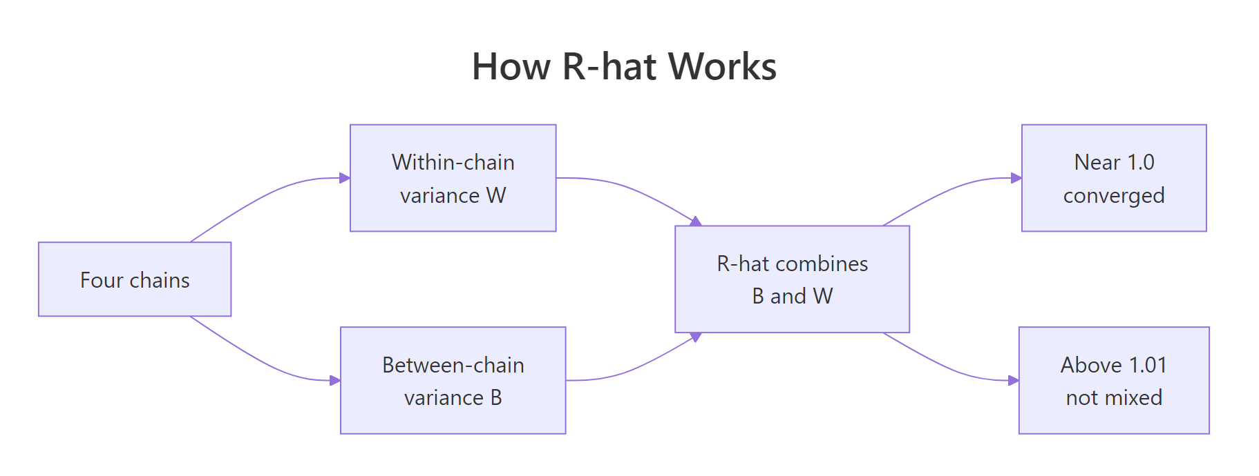
Figure 1: R-hat compares the variance between chains against the variance within them. When four chains have found the same posterior, the two variances match and the ratio sits at 1.
In practice you do not hand-roll R-hat. The posterior package computes a better version of it, so let us confirm our result with the real tool. The package is not part of base R, so this block is meant to run in your local R session (RStudio or the R console) rather than in the browser.
library(posterior)

# Wrap each matrix as a draws_array: iterations x chains x one parameter "mu"
good_draws  <- as_draws_array(array(good_post,  dim = c(nrow(good_post),  4, 1),
                                    dimnames = list(NULL, NULL, "mu")))
stuck_draws <- as_draws_array(array(stuck_post, dim = c(nrow(stuck_post), 4, 1),
                                    dimnames = list(NULL, NULL, "mu")))

summarise_draws(good_draws,  "mean", "rhat")
#>   variable  mean  rhat
#>   <chr>    <dbl> <dbl>
#> 1 mu        4.81  1.00
summarise_draws(stuck_draws, "mean", "rhat")
#>   variable  mean  rhat
#>   <chr>    <dbl> <dbl>
#> 1 mu        4.61  2.23
The package agrees on the verdict: the healthy chains land at R-hat 1.00, the stuck chains at 2.23. Notice the stuck value is even higher than our hand-rolled 1.693. That is because posterior uses the rank-normalized, split version of R-hat from Vehtari and colleagues, which splits each chain in half and ranks the draws before comparing. It is strictly more sensitive to problems, so a broken chain looks even worse under it. For a healthy run the two versions agree closely; for a broken one, the improved version is quicker to raise the alarm.
Try it: A step of 0.02 was hopeless and a step of 1 was great. Check a middle value: run four chains at step = 0.3, drop the warmup, and see whether R-hat clears the 1.01 bar.
Click to reveal solution
Explanation: A step of 0.3 gives R-hat 1.004, just under the 1.01 threshold, so the four chains did reach agreement. It passes, but only barely. As we are about to see, passing R-hat is necessary but not sufficient; you still have to check how much information those chains carry.
How does effective sample size measure wasted draws?
R-hat tells you the chains agree with each other. It does not tell you whether they explored efficiently. A chain can pass R-hat while producing draws that are almost copies of one another, and near-copies carry very little information. Effective sample size, usually written ESS, is the count that corrects for this. It answers a blunt question: your chain has 2000 draws, but how many genuinely independent draws are they worth?
The culprit is autocorrelation, the tendency of each draw to resemble the one before it. In a well-mixed chain, consecutive draws are nearly unrelated. In a poorly-mixed chain, each draw is a tiny nudge away from the last, so neighboring draws are almost identical. Let us measure it directly with acf(), which reports the correlation between draws separated by a given lag.
In the healthy chain, the correlation at lag 1 is 0.622 and it decays quickly toward zero: draws a few steps apart are already fairly independent. In the stuck chain, the correlation is 0.998 at lag 1 and barely falls at all, because each draw is almost exactly the previous one. Draws that similar are close to useless as fresh evidence. The formula for effective sample size turns that decay curve into a number.
$$N_{\text{eff}} = \frac{N}{1 + 2\sum_{k=1}^{\infty}\rho_k}$$
Where $N$ is the total number of draws and $\rho_k$ is the autocorrelation at lag $k$. When the correlations are near zero, the denominator is close to 1 and effective sample size roughly equals the raw count. When the correlations stay high, the denominator balloons and effective sample size collapses. Here is that calculation in code, summing the autocorrelations until they turn negative.
One healthy chain of 2000 draws is worth about 354 independent draws. That is the real cost of autocorrelation: you paid for 2000, you got the information content of 354. The stuck chain is far worse. Its 2000 draws are worth 3.5 independent draws, essentially nothing. A chain that barely moves gives you almost no information no matter how long you run it.
The posterior package computes two refined versions of this: bulk-ESS, which measures information about the center of the distribution, and tail-ESS, which measures information in the tails where the extreme quantiles live. Both matter, because a chain can pin down the mean well while still being shaky about a 95% interval. This block also runs locally.
summarise_draws(good_draws,  "ess_bulk", "ess_tail")
#>   variable ess_bulk ess_tail
#>   <chr>       <dbl>    <dbl>
#> 1 mu          1594.    1788.
summarise_draws(stuck_draws, "ess_bulk", "ess_tail")
#>   variable ess_bulk ess_tail
#>   <chr>       <dbl>    <dbl>
#> 1 mu           5.09     11.7
Across all four healthy chains, bulk-ESS is about 1594 and tail-ESS about 1788, comfortable numbers. The stuck chains manage a bulk-ESS of 5 and a tail-ESS of 12, which is a disaster. The standard rule of thumb is to want at least 400 effective draws for each of bulk and tail before you report a quantity, since 400 is roughly where Monte Carlo error becomes negligible for typical summaries.
Try it: The medium step of 0.3 passed R-hat. Check its effective sample size with ess_basic() on the first medium-step chain. Does a single chain clear the 400 mark?
Click to reveal solution
Explanation: A single medium-step chain is worth about 177 effective draws, under the 400 floor on its own. Pooled across four chains it clears 400, which is why running several chains helps: each contributes its own effective draws to the total. The medium step is workable but not efficient, and the well-tuned step of 1 is clearly better.
What do healthy and unhealthy trace plots look like?
Numbers are decisive, but a trained eye catches problems in seconds, and the trace plot is the tool for that. A trace plot draws each chain's value against the iteration number. A healthy chain looks like a fat fuzzy caterpillar with no trend, and when you overlay several chains they sit on top of one another. An unhealthy chain shows one of a few tell-tale shapes: a slow drift up or down (it is still traveling, not exploring), long flat stretches (it is stuck, rejecting every move), or several chains parked in separate horizontal bands (they never came together). Let us overlay the four chains for each case.
The healthy plot is a single blur: all four chains occupy the same band around 4.8, weaving through each other constantly. That overlap is the visual signature of convergence. The stuck plot shows four distinct ribbons that never touch, each chain sitting near where it started. You would not need R-hat to know the second run failed; your eyes catch it instantly.
There is a sharper cousin of the trace plot called the rank plot. Instead of raw values, you rank every draw across all chains pooled together, then histogram the ranks within each chain. If the chains are interchangeable, every chain should hold an even mix of low, middle, and high ranks, so each histogram is flat. A chain sitting too high or too low shows up as a lopsided histogram. Rank plots are easier to read than trace plots when you have many chains or very high autocorrelation.
For the healthy chains, the four rank histograms are roughly flat, each chain holding its fair share of low and high ranks. For the stuck chains, the histograms are badly lopsided: chain 1 holds mostly low ranks (it sat near 3.9), chain 4 holds mostly high ranks (it sat near 5.3). A flat rank histogram is what convergence looks like from this angle.
If you work with fitted Stan models, the bayesplot package draws both of these with one call each. It is a local-only package, so treat this as run-locally code.
library(bayesplot)

mcmc_trace(good_draws)         # overlaid trace plot in one call
mcmc_rank_overlay(good_draws) # overlaid rank plot in one callTry it: Overlay the four medium-step chains from earlier. Do they pile on top of each other like the healthy set, or sit in separate bands like the stuck set?
Click to reveal solution
Explanation: The medium-step chains overlap far more than the stuck ones, which matches its passing R-hat of 1.004. Look closely and you can see a lazier, wider wander than the crisp step-of-1 chains, the visual fingerprint of its lower effective sample size.
What are divergences, and why do they matter?
Everything so far applies to any sampler. R-hat, effective sample size, and trace plots work on draws no matter how you produced them. Real Bayesian models, though, are almost never fit with the plain Metropolis sampler we built. They are fit with Hamiltonian Monte Carlo (HMC), the engine inside Stan, rstanarm, and brms. HMC is faster and smarter, and it comes with one extra diagnostic that our toy sampler has no version of: the divergence.
Before we get to divergences, let us see the familiar diagnostics on a model you would actually fit. We will fit an ordinary linear regression with rstanarm, which runs HMC under the hood and reports R-hat and effective sample size for every parameter automatically. rstanarm uses precompiled models and is not a browser package, so run this locally.
library(rstanarm)

set.seed(2024)
fit <- stan_glm(mpg ~ wt + am, data = mtcars,
                chains = 4, iter = 1000, refresh = 0, seed = 2024)

params <- c("(Intercept)", "wt", "am", "sigma")
round(summary(fit)[params, c("mean", "sd", "n_eff", "Rhat")], 3)
#>               mean    sd n_eff  Rhat
#> (Intercept) 37.247 3.199   617 1.006
#> wt          -5.332 0.824   676 1.004
#> am           0.020 1.634   739 1.003
#> sigma        3.201 0.418  1141 1.007
The summary reports exactly the two diagnostics we built. Here n_eff is effective sample size and Rhat is R-hat, printed for each parameter. Every R-hat sits at or below 1.007 and every n_eff clears 400, so this fit converged. The same reasoning you learned on the toy problem reads a production model unchanged.
A divergence is HMC's own alarm. HMC works by simulating a frictionless particle rolling across the posterior surface. When the surface has a region of extreme curvature, a narrow funnel where the density changes very fast, the simulation becomes numerically unstable and the particle shoots off course. Stan detects that failure and records it as a divergent transition. Divergences tend to cluster in the same troublesome region, so even a handful of them means the sampler is systematically avoiding part of the posterior, and your estimates there cannot be trusted. Checking the count is one line.
rstan::get_num_divergent(fit$stanfit)
#> [1] 0
Zero divergences, as expected for a simple regression. When the count is not zero, two fixes handle most cases. First, make the sampler more careful by raising adapt_delta toward 1, for example control = list(adapt_delta = 0.99), which forces smaller, safer steps at the cost of speed. Second, reparameterize the model so the funnel geometry goes away, the classic move being the non-centered parameterization for hierarchical models. Reparameterization fixes the cause; raising adapt_delta treats the symptom, and is the quick first thing to try.
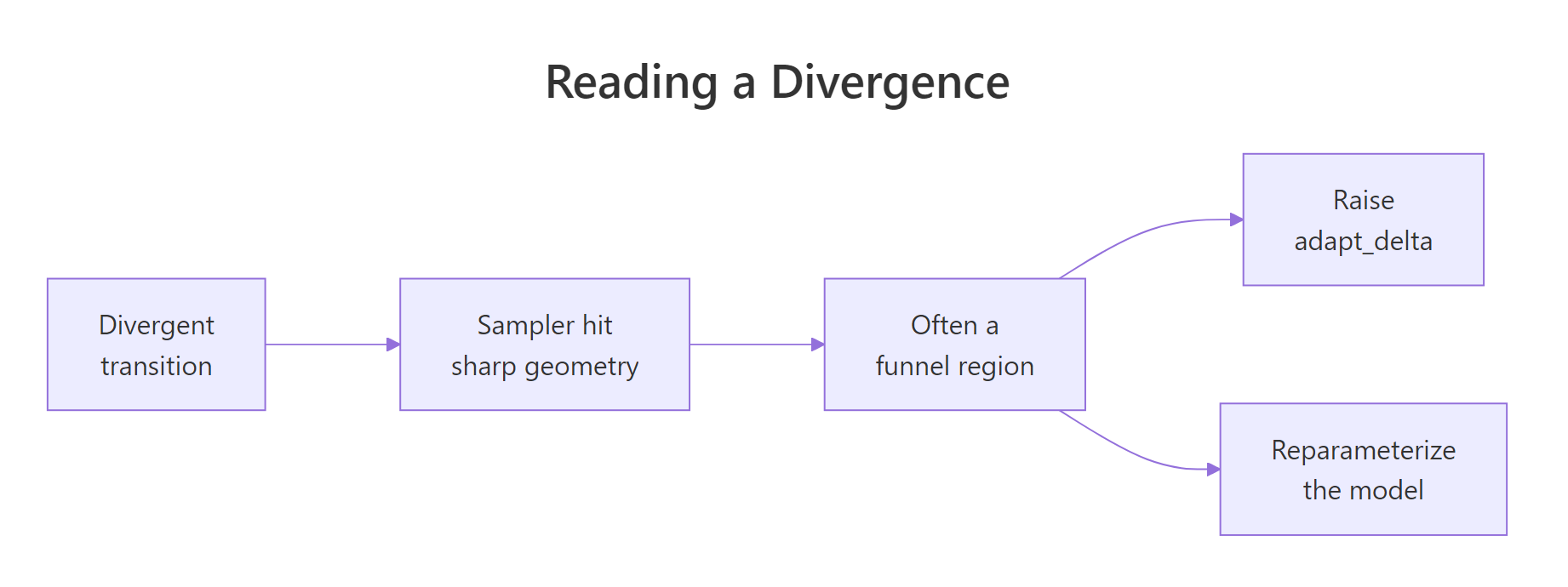
Figure 2: A divergence means the HMC sampler hit a region of sharp geometry, usually a funnel. The two standard responses are a more careful sampler (higher adapt_delta) or a reparameterized model.
Try it: Our Metropolis sampler has no divergences, but it has a related symptom: a stuck chain rejects almost every move, so it repeats the same value over and over. Measure how often the stuck chain failed to move by counting iterations where the value did not change.
Click to reveal solution
Explanation: About 6% of the stuck chain's steps were outright rejections where it stayed put. That is not the whole story, since even its accepted moves are microscopic, but it is the plainest sign a chain is struggling to move, the random-walk cousin of a divergence.
How do you fix a chain that fails its diagnostics?
Diagnostics are only useful if you know what to do when they fail. The workflow is a short loop: diagnose the problem, adjust one knob, re-run, and re-check. You repeat until every diagnostic passes. The knobs you have are the step size, the warmup length, the total number of iterations, the priors, and, for hard models, the parameterization. Let us walk the whole loop on the stuck run.
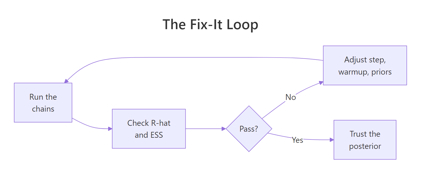
Figure 3: The fix-it loop. Run the chains, check R-hat and ESS, and if either fails, adjust a knob and run again. Only trust the posterior once both pass.
First, restate the diagnosis so we know what we are fixing. The stuck run fails on both counts.
R-hat 1.69 and an effective sample size of 3.5 both scream failure. The root cause here is the step size, so that is the knob to turn. We raise it from 0.02 back to 1, and while we are at it we run longer and warm up longer, giving the chains room to settle. Then we re-check.
R-hat drops to 1.0004, and each chain now carries roughly 900 effective draws. Both diagnostics pass. The final step of any fix is to confirm the answer against something you trust, and here we are lucky enough to have the closed-form posterior mean.
The repaired chain estimates 4.81 against the true 4.801, a match to two decimal places. The loop worked: one bad knob, one adjustment, a clean re-check.
Try it: Is bigger always better? Redo the fix with an even larger step of 2 and compare its R-hat and effective sample size to the step-of-1 run above.
Click to reveal solution
Explanation: The step of 2 still converges (R-hat 1.002), but its average effective sample size falls to about 642, below the roughly 930 the step of 1 delivered. Too large a step gets rejected too often, which raises autocorrelation. There is a sweet spot, and overshooting it costs efficiency just like undershooting does.
Practice Exercises
Exercise 1: Judge a borderline run
Run four chains at step = 0.1, drop the 2000-iteration warmup, and report both R-hat and the four per-chain effective sample sizes. Then make the call: does this run pass the bar of R-hat below 1.01 and ESS above 400?
Click to reveal solution
Explanation: This run fails both bars. R-hat is 1.033, above 1.01, and each chain carries only 20 to 37 effective draws, far below 400. A step of 0.1 is still too small for a posterior this narrow (its standard deviation is only 0.4), so the chains crawl. The verdict is a clear reject: do not report anything from this run.
Exercise 2: Write a one-shot verdict function
Write diagnose(chains) that drops the warmup, computes R-hat with rhat_basic(), sums the effective sample sizes across chains with ess_basic(), and returns "PASS" only when R-hat is below 1.01 and total ESS is above 400. Test it on the good and stuck4 matrices.
Click to reveal solution
Explanation: The good matrix passes with R-hat 1.002 and about 1581 total effective draws. The stuck matrix fails with R-hat 1.693 and only 24 effective draws. Bundling the two checks into one function is exactly what production diagnostics do: a single call, a single verdict, no room to forget one of the tests.
Exercise 3: Can brute force rescue a stuck chain?
A tempting claim: the stuck chains were not broken, just slow, so running them much longer should fix everything. Test it. Run the step = 0.02 chains ten times longer (n_iter = 40000), drop a 20000-iteration warmup, and re-check R-hat. Does raw iteration count alone get you under 1.01?
Click to reveal solution
Explanation: Ten times the iterations dragged R-hat from 1.69 down to 1.141, a real improvement, and the chain means are closer together than before. But 1.141 is still nowhere near the 1.01 bar, and the chains still disagree. This is the lesson from the fix-it section made concrete: brute force helps a badly-tuned sampler slowly and expensively, while retuning the step size fixed the same problem in one shot. Fix the mixing, do not just wait it out.
Complete Example: A full convergence report on fresh data
Let us put the whole workflow together on a dataset we have not seen, exactly as you would in real work: simulate the data, run several chains, produce a one-glance report of R-hat, total effective sample size, and the posterior mean, then sanity-check against the closed form. The sampler machinery is unchanged; we just point it at a new target by passing a new log-posterior.
The report is clean: R-hat is 1.0001, total effective sample size is 2614, and the posterior mean is 2.114. The closed-form posterior mean for this new data is 2.131, so the sampled estimate matches the truth to within ordinary Monte Carlo error. This is the shape of every real convergence check you will run. Fit the model, read R-hat and effective sample size, and only report the estimate once both pass. When you have a ground truth to compare against, use it; when you do not, the diagnostics are your only assurance, which is exactly why they matter.
Frequently Asked Questions
How many chains should I run? Four is the standard default, and it is what Stan and rstanarm use out of the box. R-hat needs at least two chains to have anything to compare, but two is too few to spot a chain stuck on a lonely mode. Four gives you a reliable read without much extra cost, and running them is cheap since they are independent.
What R-hat and ESS values are actually safe? Aim for R-hat below 1.01 for every parameter and at least 400 for both bulk-ESS and tail-ESS on any quantity you report. These come from Vehtari et al. (2021). Older sources say R-hat below 1.1, which is now considered too lenient; the stricter bar catches problems the old one misses.
My R-hat passes but ESS is low. Is that a problem? Yes. They diagnose different failures. A low ESS with a good R-hat means all your chains agree but move so slowly that they carry little information. Your posterior summaries will be noisy. The usual fix is better sampler tuning, not simply more iterations.
What is the difference between bulk-ESS and tail-ESS? Bulk-ESS measures how much information the draws carry about the center of the distribution, such as the mean or median. Tail-ESS measures information in the extremes, which is what you need for reliable 90% or 95% intervals. A chain can be fine in the bulk and shaky in the tails, so check both.
Do these diagnostics work for my own hand-written sampler, or only for Stan? R-hat, effective sample size, and trace plots work on any set of draws, whoever produced them, which is why we could compute them on a plain Metropolis chain. Divergences are the one exception: they are specific to Hamiltonian Monte Carlo, so they appear only with Stan-family tools.
Summary
The four diagnostics in this post answer one question from four angles: has this run actually explored the posterior? Read them together, never alone.
| Diagnostic | What it checks | Healthy value | Tool |
|---|---|---|---|
| R-hat | Do multiple chains agree? | Below 1.01 | posterior::summarise_draws |
| Effective sample size | How much independent information? | Above 400 | posterior::summarise_draws |
| Trace and rank plots | Any visible pathology? | Fuzzy overlap, flat ranks | bayesplot::mcmc_trace |
| Divergences | Did HMC hit broken geometry? | Zero | rstan::get_num_divergent |
The workflow is always the same loop. Run several chains from dispersed starts, drop the warmup, compute R-hat and effective sample size, glance at the trace and rank plots, and for HMC fits check the divergence count. If anything fails, adjust one knob, usually the step size or the parameterization, then re-run and re-check. Only when every diagnostic passes are the draws a fair picture of the posterior.
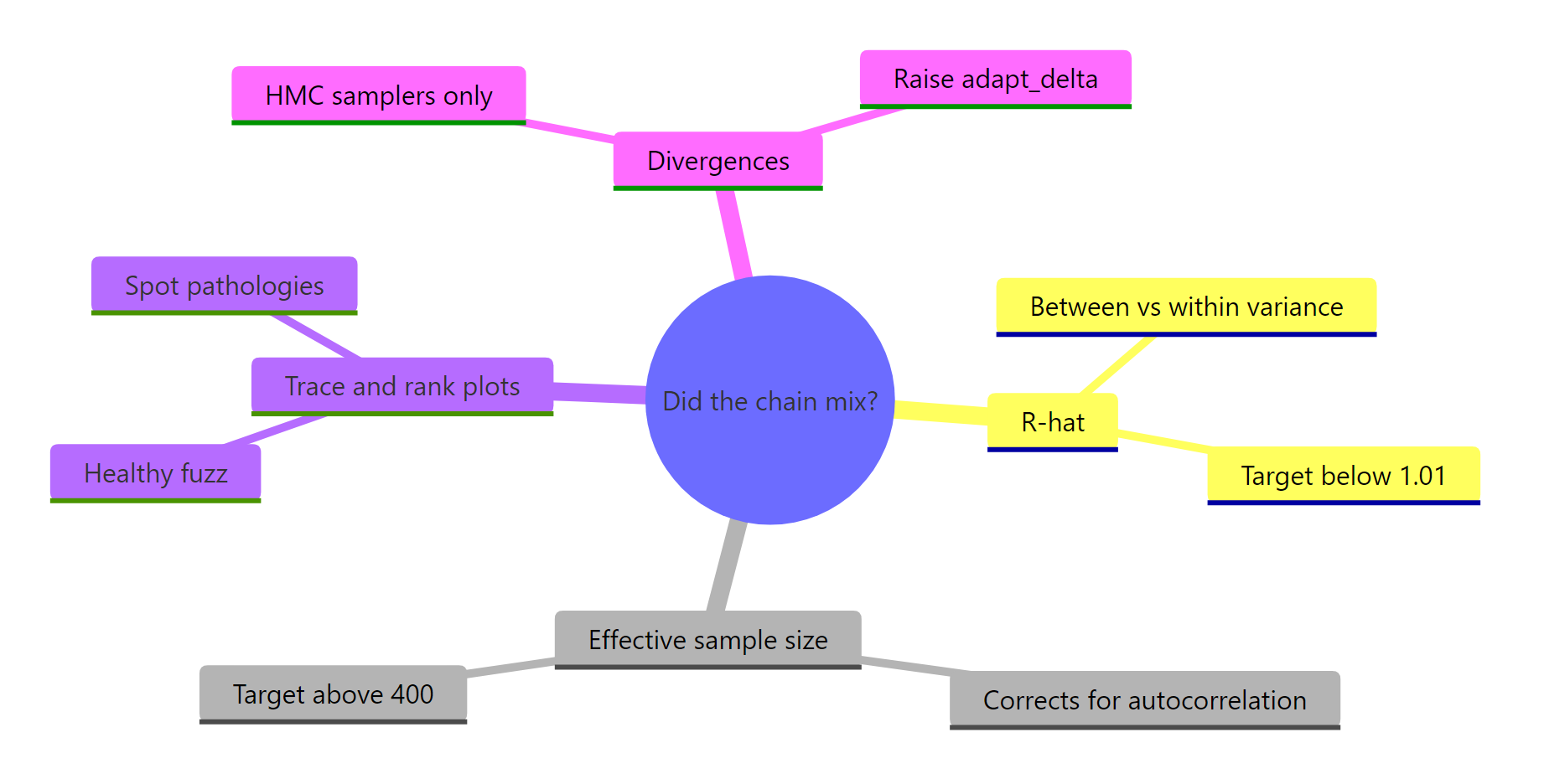
Figure 4: The four convergence diagnostics at a glance. Each one asks whether the chain mixed; together they cover the ways a run can fail.
References
- Vehtari, A., Gelman, A., Simpson, D., Carpenter, B., Bürkner, P. (2021). "Rank-normalization, folding, and localization: An improved R-hat for assessing convergence of MCMC." Bayesian Analysis. Link
- posterior package documentation, Stan Development Team. Link
- bayesplot: Visual MCMC diagnostics, Stan Development Team. Link
- rstanarm: Bayesian applied regression modeling, Stan Development Team. Link
- coda: Output analysis and diagnostics for MCMC, Plummer et al. Link
- Roy, V. (2020). "Convergence diagnostics for Markov chain Monte Carlo." Annual Review of Statistics and Its Application. Link
- Stan Reference Manual, "Posterior Analysis" (R-hat, effective sample size, divergences), Stan Development Team. Link
Continue Learning
- Build MCMC From Scratch in R, the sampler this post inspects, explained line by line. Start there if the Metropolis code felt fast.
- Conjugate Priors in R, where the closed-form posterior we checked against comes from. It shows why the normal-normal model has an exact answer.
- Bayesian Statistics in R, the section opener that builds prior, likelihood, and posterior from the ground up, the context every diagnostic here assumes.