{
"cells": [
{
"cell_type": "markdown",
"metadata": {
"toc": true
},
"source": [
"Table of Contents
\n",
""
]
},
{
"cell_type": "markdown",
"metadata": {},
"source": [
"Discussion and implementation of common abstact datastructures and algorithms "
]
},
{
"cell_type": "markdown",
"metadata": {},
"source": [
"Content is heavily derived from: http://interactivepython.org/runestone/static/pythonds/index.html"
]
},
{
"cell_type": "code",
"execution_count": 35,
"metadata": {},
"outputs": [],
"source": [
"import pandas as pd\n",
"import numpy as np\n",
"import time\n",
"import matplotlib.pyplot as plt\n",
"%matplotlib inline"
]
},
{
"cell_type": "markdown",
"metadata": {
"heading_collapsed": true
},
"source": [
"# Algorithm complexity"
]
},
{
"cell_type": "markdown",
"metadata": {
"hidden": true
},
"source": [
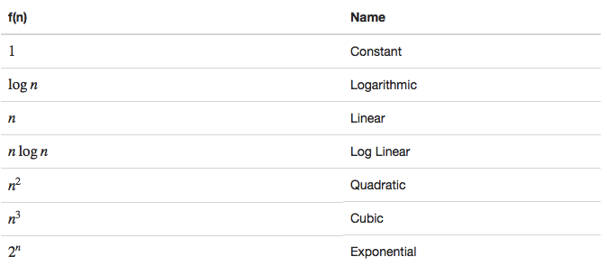
"`Big O notation` is used in Computer Science to describe the performance or complexity of an algorithm. Big O specifically describes the worst-case scenario, and can be used to describe the execution time required or the space used."
]
},
{
"cell_type": "markdown",
"metadata": {
"hidden": true
},
"source": [
"To know more: http://interactivepython.org/runestone/static/pythonds/AlgorithmAnalysis/BigONotation.html"
]
},
{
"cell_type": "markdown",
"metadata": {
"hidden": true
},
"source": [
""
]
},
{
"cell_type": "markdown",
"metadata": {
"hidden": true
},
"source": [
" "
]
},
{
"cell_type": "markdown",
"metadata": {
"hidden": true
},
"source": [
"Let's understand this through 2 different implementation of search algorithm"
]
},
{
"cell_type": "markdown",
"metadata": {
"heading_collapsed": true,
"hidden": true
},
"source": [
"## Search algorithm"
]
},
{
"cell_type": "markdown",
"metadata": {
"heading_collapsed": true,
"hidden": true
},
"source": [
"### Linear search"
]
},
{
"cell_type": "code",
"execution_count": 93,
"metadata": {
"hidden": true
},
"outputs": [],
"source": [
"def linear_search(l, target):\n",
" for e in l:\n",
" if e == target:\n",
" return True\n",
" return False"
]
},
{
"cell_type": "code",
"execution_count": 94,
"metadata": {
"hidden": true
},
"outputs": [],
"source": [
"l = np.arange(1000)"
]
},
{
"cell_type": "code",
"execution_count": 95,
"metadata": {
"hidden": true
},
"outputs": [
{
"name": "stdout",
"output_type": "stream",
"text": [
"265 µs ± 5.07 µs per loop (mean ± std. dev. of 7 runs, 1000 loops each)\n"
]
}
],
"source": [
"%%timeit\n",
"linear_search(l,999)"
]
},
{
"cell_type": "markdown",
"metadata": {
"hidden": true
},
"source": [
"Time scales linearly with n. So Big-O is $O(n)$"
]
},
{
"cell_type": "markdown",
"metadata": {
"heading_collapsed": true,
"hidden": true
},
"source": [
"### Binary search"
]
},
{
"cell_type": "markdown",
"metadata": {
"hidden": true
},
"source": [
"Iterative algo"
]
},
{
"cell_type": "code",
"execution_count": 96,
"metadata": {
"hidden": true
},
"outputs": [],
"source": [
"def binarySearchIterative(a, t):\n",
" upper = len(a) - 1\n",
" lower = 0\n",
" while lower <= upper:\n",
" middle = (lower + upper) // 2\n",
" if t == a[middle]:\n",
" return True\n",
" else:\n",
" if t < a[middle]:\n",
" upper = middle - 1\n",
" else:\n",
" lower = middle + 1\n",
" return False"
]
},
{
"cell_type": "code",
"execution_count": 97,
"metadata": {
"hidden": true
},
"outputs": [],
"source": [
"l = np.arange(1000)"
]
},
{
"cell_type": "code",
"execution_count": 98,
"metadata": {
"hidden": true
},
"outputs": [
{
"name": "stdout",
"output_type": "stream",
"text": [
"9.05 µs ± 419 ns per loop (mean ± std. dev. of 7 runs, 100000 loops each)\n"
]
}
],
"source": [
"%%timeit\n",
"binarySearchIterative(l,999)"
]
},
{
"cell_type": "markdown",
"metadata": {
"hidden": true
},
"source": [
"Time scales linearly with n. So Big-O is $O(log(n))$"
]
},
{
"cell_type": "markdown",
"metadata": {
"hidden": true
},
"source": [
"We can see that binary search is almost 30x faster"
]
},
{
"cell_type": "markdown",
"metadata": {
"hidden": true
},
"source": [
"We can do binary search in a recursive way too"
]
},
{
"cell_type": "code",
"execution_count": 100,
"metadata": {
"hidden": true
},
"outputs": [],
"source": [
"def binarySearchRecursive(a, t):\n",
" upper = len(a) - 1\n",
" lower = 0\n",
" if upper >= 0:\n",
" middle = (lower + upper) // 2\n",
" if t == a[middle]: return True\n",
" if t < a[middle]: return binarySearchRecursive(a[:middle], t)\n",
" else: return binarySearchRecursive(a[middle + 1:], t)\n",
" return False"
]
},
{
"cell_type": "code",
"execution_count": 101,
"metadata": {
"hidden": true
},
"outputs": [
{
"name": "stdout",
"output_type": "stream",
"text": [
"15.6 µs ± 517 ns per loop (mean ± std. dev. of 7 runs, 100000 loops each)\n"
]
}
],
"source": [
"%%timeit\n",
"binarySearchRecursive(l,999)"
]
},
{
"cell_type": "markdown",
"metadata": {
"heading_collapsed": true
},
"source": [
"# Sorting algorithms"
]
},
{
"cell_type": "markdown",
"metadata": {
"hidden": true
},
"source": [
"Source: http://interactivepython.org/runestone/static/pythonds/SortSearch/toctree.html"
]
},
{
"cell_type": "markdown",
"metadata": {
"heading_collapsed": true,
"hidden": true
},
"source": [
"### Bubble sort"
]
},
{
"cell_type": "markdown",
"metadata": {
"hidden": true
},
"source": [
""
]
},
{
"cell_type": "markdown",
"metadata": {
"hidden": true
},
"source": [
"$$Complexity: O(n^2)$$"
]
},
{
"cell_type": "markdown",
"metadata": {
"hidden": true
},
"source": [
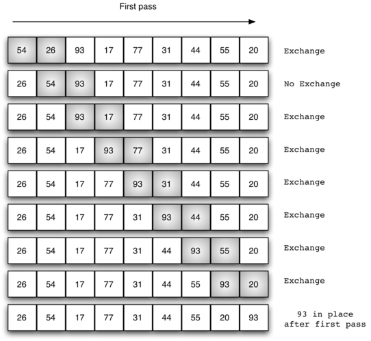
"A bubble sort is often considered the most inefficient sorting method since it must exchange items before the final location is known. These “wasted” exchange operations are very costly. However, because the bubble sort makes passes through the entire unsorted portion of the list, it has the capability to do something most sorting algorithms cannot. In particular, if during a pass there are no exchanges, then we know that the list must be sorted. A bubble sort can be modified to stop early if it finds that the list has become sorted. This means that for lists that require just a few passes, a bubble sort may have an advantage in that it will recognize the sorted list and stop."
]
},
{
"cell_type": "code",
"execution_count": 589,
"metadata": {
"hidden": true
},
"outputs": [],
"source": [
"l = [1,2,3,4,32,5,5,66,33,221,34,23,12]"
]
},
{
"cell_type": "code",
"execution_count": 590,
"metadata": {
"hidden": true
},
"outputs": [],
"source": [
"def bubblesort(nums):\n",
" n = len(nums)\n",
" exchange_cnt = 1\n",
" while exchange_cnt > 0:\n",
" exchange_cnt = 0\n",
" for i in range(1, n):\n",
" if nums[i] < nums[i - 1]:\n",
" exchange_cnt += 1\n",
" nums[i - 1], nums[i] = nums[i], nums[i - 1]\n",
" print(nums)\n",
" return nums"
]
},
{
"cell_type": "code",
"execution_count": 591,
"metadata": {
"hidden": true
},
"outputs": [
{
"name": "stdout",
"output_type": "stream",
"text": [
"[1, 2, 3, 4, 5, 5, 32, 33, 66, 34, 23, 12, 221]\n",
"[1, 2, 3, 4, 5, 5, 32, 33, 34, 23, 12, 66, 221]\n",
"[1, 2, 3, 4, 5, 5, 32, 33, 23, 12, 34, 66, 221]\n",
"[1, 2, 3, 4, 5, 5, 32, 23, 12, 33, 34, 66, 221]\n",
"[1, 2, 3, 4, 5, 5, 23, 12, 32, 33, 34, 66, 221]\n",
"[1, 2, 3, 4, 5, 5, 12, 23, 32, 33, 34, 66, 221]\n",
"[1, 2, 3, 4, 5, 5, 12, 23, 32, 33, 34, 66, 221]\n"
]
},
{
"data": {
"text/plain": [
"[1, 2, 3, 4, 5, 5, 12, 23, 32, 33, 34, 66, 221]"
]
},
"execution_count": 591,
"metadata": {},
"output_type": "execute_result"
}
],
"source": [
"bubblesort(l)"
]
},
{
"cell_type": "markdown",
"metadata": {
"heading_collapsed": true,
"hidden": true
},
"source": [
"### Selection sort"
]
},
{
"cell_type": "markdown",
"metadata": {
"hidden": true
},
"source": [
""
]
},
{
"cell_type": "markdown",
"metadata": {
"hidden": true
},
"source": [
"$$Complexity: O(n^2)$$"
]
},
{
"cell_type": "markdown",
"metadata": {
"hidden": true
},
"source": [
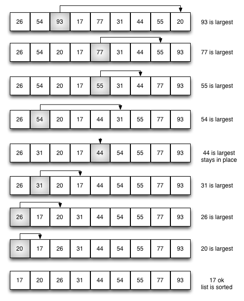
"The selection sort improves on the bubble sort by making only one exchange for every pass through the list. In order to do this, a selection sort looks for the largest value as it makes a pass and, after completing the pass, places it in the proper location. As with a bubble sort, after the first pass, the largest item is in the correct place. After the second pass, the next largest is in place. This process continues and requires n−1 passes to sort n items, since the final item must be in place after the (n−1) st pass."
]
},
{
"cell_type": "code",
"execution_count": 46,
"metadata": {
"hidden": true
},
"outputs": [],
"source": [
"l = [1,2,3,4,32,5,5,66,33,221,34,23,12]"
]
},
{
"cell_type": "code",
"execution_count": 39,
"metadata": {
"hidden": true
},
"outputs": [],
"source": [
"def selectionSort(l):\n",
" n = len(l)\n",
" end = n - 1\n",
" for j in range(n):\n",
" max_ = l[-1 - j]\n",
" max_idx = -1 - j\n",
" for i in range(end):\n",
" if l[i] > max_:\n",
" max_ = l[i]\n",
" max_idx = i\n",
" else:\n",
" continue\n",
" l[-1 - j], l[max_idx] = l[max_idx], l[-1 - j]\n",
" end = end - 1\n",
" print(l)\n",
" return l"
]
},
{
"cell_type": "code",
"execution_count": 40,
"metadata": {
"hidden": true
},
"outputs": [
{
"name": "stdout",
"output_type": "stream",
"text": [
"[1, 2, 3, 4, 32, 5, 5, 66, 33, 12, 34, 23, 221]\n",
"[1, 2, 3, 4, 32, 5, 5, 23, 33, 12, 34, 66, 221]\n",
"[1, 2, 3, 4, 32, 5, 5, 23, 33, 12, 34, 66, 221]\n",
"[1, 2, 3, 4, 32, 5, 5, 23, 12, 33, 34, 66, 221]\n",
"[1, 2, 3, 4, 12, 5, 5, 23, 32, 33, 34, 66, 221]\n",
"[1, 2, 3, 4, 12, 5, 5, 23, 32, 33, 34, 66, 221]\n",
"[1, 2, 3, 4, 5, 5, 12, 23, 32, 33, 34, 66, 221]\n",
"[1, 2, 3, 4, 5, 5, 12, 23, 32, 33, 34, 66, 221]\n",
"[1, 2, 3, 4, 5, 5, 12, 23, 32, 33, 34, 66, 221]\n",
"[1, 2, 3, 4, 5, 5, 12, 23, 32, 33, 34, 66, 221]\n",
"[1, 2, 3, 4, 5, 5, 12, 23, 32, 33, 34, 66, 221]\n",
"[1, 2, 3, 4, 5, 5, 12, 23, 32, 33, 34, 66, 221]\n",
"[1, 2, 3, 4, 5, 5, 12, 23, 32, 33, 34, 66, 221]\n"
]
},
{
"data": {
"text/plain": [
"[1, 2, 3, 4, 5, 5, 12, 23, 32, 33, 34, 66, 221]"
]
},
"execution_count": 40,
"metadata": {},
"output_type": "execute_result"
}
],
"source": [
"selectionSort(l)"
]
},
{
"cell_type": "markdown",
"metadata": {
"hidden": true
},
"source": [
"The benefit of selection over bubble sort is it does one exchange per pass whereas bubble sort can do multiple exchanges."
]
},
{
"cell_type": "markdown",
"metadata": {
"heading_collapsed": true,
"hidden": true
},
"source": [
"### Insertion sort"
]
},
{
"cell_type": "markdown",
"metadata": {
"hidden": true
},
"source": [
""
]
},
{
"cell_type": "markdown",
"metadata": {
"hidden": true
},
"source": [
"$$Complexity: O(n^2)$$"
]
},
{
"cell_type": "code",
"execution_count": 605,
"metadata": {
"hidden": true
},
"outputs": [],
"source": [
"l = [1,2,3,4,32,5,5,66,33,221,34,23,12]"
]
},
{
"cell_type": "code",
"execution_count": 606,
"metadata": {
"hidden": true
},
"outputs": [],
"source": [
"def insertionSort(l):\n",
" for i in range(1, len(l)):\n",
" cval = l[i]\n",
" pos = i\n",
" while pos > 0 and l[pos - 1] > cval:\n",
" l[pos],l[pos-1] = l[pos - 1],l[pos]\n",
" pos = pos - 1\n",
" print(l)\n",
" return l"
]
},
{
"cell_type": "code",
"execution_count": 607,
"metadata": {
"hidden": true
},
"outputs": [
{
"name": "stdout",
"output_type": "stream",
"text": [
"[1, 2, 3, 4, 32, 5, 5, 66, 33, 221, 34, 23, 12]\n",
"[1, 2, 3, 4, 32, 5, 5, 66, 33, 221, 34, 23, 12]\n",
"[1, 2, 3, 4, 32, 5, 5, 66, 33, 221, 34, 23, 12]\n",
"[1, 2, 3, 4, 32, 5, 5, 66, 33, 221, 34, 23, 12]\n",
"[1, 2, 3, 4, 5, 32, 5, 66, 33, 221, 34, 23, 12]\n",
"[1, 2, 3, 4, 5, 5, 32, 66, 33, 221, 34, 23, 12]\n",
"[1, 2, 3, 4, 5, 5, 32, 66, 33, 221, 34, 23, 12]\n",
"[1, 2, 3, 4, 5, 5, 32, 33, 66, 221, 34, 23, 12]\n",
"[1, 2, 3, 4, 5, 5, 32, 33, 66, 221, 34, 23, 12]\n",
"[1, 2, 3, 4, 5, 5, 32, 33, 34, 66, 221, 23, 12]\n",
"[1, 2, 3, 4, 5, 5, 23, 32, 33, 34, 66, 221, 12]\n",
"[1, 2, 3, 4, 5, 5, 12, 23, 32, 33, 34, 66, 221]\n"
]
},
{
"data": {
"text/plain": [
"[1, 2, 3, 4, 5, 5, 12, 23, 32, 33, 34, 66, 221]"
]
},
"execution_count": 607,
"metadata": {},
"output_type": "execute_result"
}
],
"source": [
"insertionSort(l)"
]
},
{
"cell_type": "markdown",
"metadata": {
"heading_collapsed": true,
"hidden": true
},
"source": [
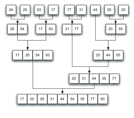
"### Merge Sort"
]
},
{
"cell_type": "markdown",
"metadata": {
"hidden": true
},
"source": [
""
]
},
{
"cell_type": "markdown",
"metadata": {
"hidden": true
},
"source": [
""
]
},
{
"cell_type": "markdown",
"metadata": {
"hidden": true
},
"source": [
"$$Complexity: O(nlog(n))$$"
]
},
{
"cell_type": "code",
"execution_count": 1,
"metadata": {
"hidden": true
},
"outputs": [],
"source": [
"l = [1,2,3,4,32,5,5,66,33,221,34,23,12]"
]
},
{
"cell_type": "code",
"execution_count": 2,
"metadata": {
"hidden": true
},
"outputs": [],
"source": [
"def mergeSort(alist):\n",
" print(\"Splitting \", alist)\n",
" if len(alist) > 1:\n",
" mid = len(alist) // 2\n",
" lefthalf = alist[:mid]\n",
" righthalf = alist[mid:]\n",
"\n",
" mergeSort(lefthalf)\n",
" mergeSort(righthalf)\n",
"\n",
" i = 0\n",
" j = 0\n",
" k = 0\n",
" while i < len(lefthalf) and j < len(righthalf):\n",
" if lefthalf[i] < righthalf[j]:\n",
" alist[k] = lefthalf[i]\n",
" i = i + 1\n",
" else:\n",
" alist[k] = righthalf[j]\n",
" j = j + 1\n",
" k = k + 1\n",
"\n",
" while i < len(lefthalf):\n",
" alist[k] = lefthalf[i]\n",
" i = i + 1\n",
" k = k + 1\n",
"\n",
" while j < len(righthalf):\n",
" alist[k] = righthalf[j]\n",
" j = j + 1\n",
" k = k + 1\n",
" print(\"Merging \", alist)"
]
},
{
"cell_type": "code",
"execution_count": 3,
"metadata": {
"hidden": true
},
"outputs": [
{
"name": "stdout",
"output_type": "stream",
"text": [
"Splitting [1, 2, 3, 4, 32, 5, 5, 66, 33, 221, 34, 23, 12]\n",
"Splitting [1, 2, 3, 4, 32, 5]\n",
"Splitting [1, 2, 3]\n",
"Splitting [1]\n",
"Merging [1]\n",
"Splitting [2, 3]\n",
"Splitting [2]\n",
"Merging [2]\n",
"Splitting [3]\n",
"Merging [3]\n",
"Merging [2, 3]\n",
"Merging [1, 2, 3]\n",
"Splitting [4, 32, 5]\n",
"Splitting [4]\n",
"Merging [4]\n",
"Splitting [32, 5]\n",
"Splitting [32]\n",
"Merging [32]\n",
"Splitting [5]\n",
"Merging [5]\n",
"Merging [5, 32]\n",
"Merging [4, 5, 32]\n",
"Merging [1, 2, 3, 4, 5, 32]\n",
"Splitting [5, 66, 33, 221, 34, 23, 12]\n",
"Splitting [5, 66, 33]\n",
"Splitting [5]\n",
"Merging [5]\n",
"Splitting [66, 33]\n",
"Splitting [66]\n",
"Merging [66]\n",
"Splitting [33]\n",
"Merging [33]\n",
"Merging [33, 66]\n",
"Merging [5, 33, 66]\n",
"Splitting [221, 34, 23, 12]\n",
"Splitting [221, 34]\n",
"Splitting [221]\n",
"Merging [221]\n",
"Splitting [34]\n",
"Merging [34]\n",
"Merging [34, 221]\n",
"Splitting [23, 12]\n",
"Splitting [23]\n",
"Merging [23]\n",
"Splitting [12]\n",
"Merging [12]\n",
"Merging [12, 23]\n",
"Merging [12, 23, 34, 221]\n",
"Merging [5, 12, 23, 33, 34, 66, 221]\n",
"Merging [1, 2, 3, 4, 5, 5, 12, 23, 32, 33, 34, 66, 221]\n"
]
}
],
"source": [
"mergeSort(l)"
]
},
{
"cell_type": "markdown",
"metadata": {
"heading_collapsed": true,
"hidden": true
},
"source": [
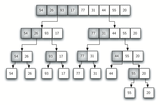
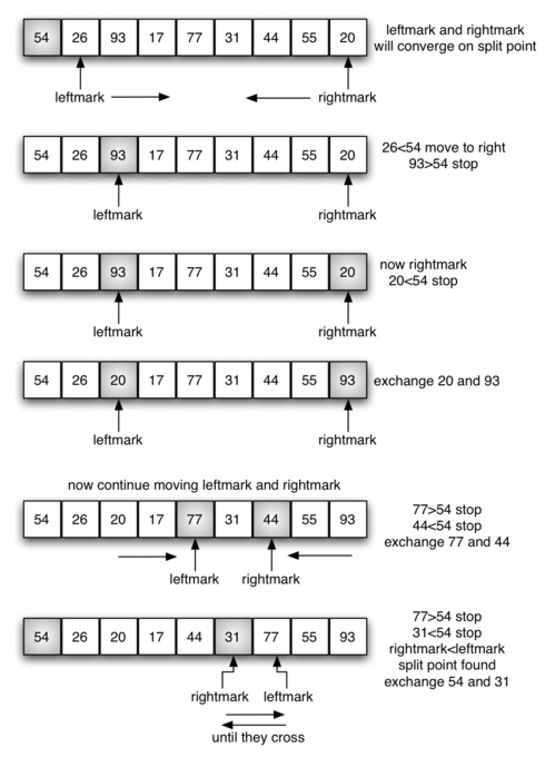
"### Quick sort"
]
},
{
"cell_type": "markdown",
"metadata": {
"hidden": true
},
"source": [
""
]
},
{
"cell_type": "markdown",
"metadata": {
"hidden": true
},
"source": [
"$$Complexity: O(nlog(n))$$ $$Worst case : O(n^2)$$"
]
},
{
"cell_type": "code",
"execution_count": 57,
"metadata": {
"hidden": true
},
"outputs": [
{
"name": "stdout",
"output_type": "stream",
"text": [
"[17, 20, 26, 31, 44, 54, 55, 77, 93]\n"
]
}
],
"source": [
"def quickSort(alist):\n",
" quickSortHelper(alist, 0, len(alist) - 1)\n",
"\n",
"\n",
"def quickSortHelper(alist, first, last):\n",
" if first < last:\n",
"\n",
" splitpoint = partition(alist, first, last)\n",
"\n",
" quickSortHelper(alist, first, splitpoint - 1)\n",
" quickSortHelper(alist, splitpoint + 1, last)\n",
"\n",
"\n",
"def partition(alist, first, last):\n",
" pivotvalue = alist[first]\n",
"\n",
" leftmark = first + 1\n",
" rightmark = last\n",
"\n",
" done = False\n",
" while not done:\n",
"\n",
" while leftmark <= rightmark and alist[leftmark] <= pivotvalue:\n",
" leftmark = leftmark + 1\n",
"\n",
" while alist[rightmark] >= pivotvalue and rightmark >= leftmark:\n",
" rightmark = rightmark - 1\n",
"\n",
" if rightmark < leftmark:\n",
" done = True\n",
" else:\n",
" temp = alist[leftmark]\n",
" alist[leftmark] = alist[rightmark]\n",
" alist[rightmark] = temp\n",
"\n",
" temp = alist[first]\n",
" alist[first] = alist[rightmark]\n",
" alist[rightmark] = temp\n",
"\n",
" return rightmark\n",
"\n",
"\n",
"alist = [54, 26, 93, 17, 77, 31, 44, 55, 20]\n",
"quickSort(alist)\n",
"print(alist)"
]
},
{
"cell_type": "markdown",
"metadata": {},
"source": [
"# Data structures"
]
},
{
"cell_type": "markdown",
"metadata": {},
"source": [
"Linear structures:\n",
"We will begin our study of data structures by considering four simple but very powerful concepts. Stacks, queues, and linked lists are examples of data collections whose items are ordered depending on how they are added or removed. Once an item is added, it stays in that position relative to the other elements that came before and came after it. Collections such as these are often referred to as linear data structures.http://interactivepython.org/runestone/static/pythonds/BasicDS/WhatAreLinearStructures.html"
]
},
{
"cell_type": "markdown",
"metadata": {},
"source": [
"## Stack"
]
},
{
"cell_type": "markdown",
"metadata": {},
"source": [
"http://interactivepython.org/runestone/static/pythonds/BasicDS/WhatisaStack.html"
]
},
{
"cell_type": "markdown",
"metadata": {},
"source": [
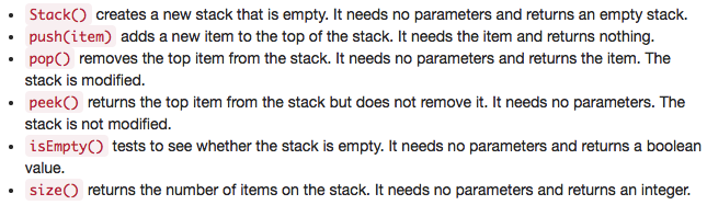
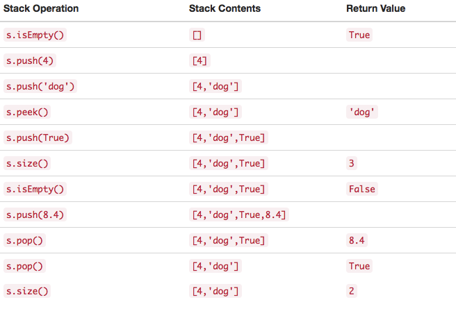
"A stack (sometimes called a “push-down stack”) is an ordered collection of items where the addition of new items and the removal of existing items always takes place at the same end. This end is commonly referred to as the “top.” The end opposite the top is known as the “base.”\n",
"\n",
"The base of the stack is significant since items stored in the stack that are closer to the base represent those that have been in the stack the longest. The most recently added item is the one that is in position to be removed first. This ordering principle is sometimes called LIFO, last-in first-out. It provides an ordering based on length of time in the collection. Newer items are near the top, while older items are near the base"
]
},
{
"cell_type": "markdown",
"metadata": {},
"source": [
"
"
]
},
{
"cell_type": "markdown",
"metadata": {
"hidden": true
},
"source": [
"Let's understand this through 2 different implementation of search algorithm"
]
},
{
"cell_type": "markdown",
"metadata": {
"heading_collapsed": true,
"hidden": true
},
"source": [
"## Search algorithm"
]
},
{
"cell_type": "markdown",
"metadata": {
"heading_collapsed": true,
"hidden": true
},
"source": [
"### Linear search"
]
},
{
"cell_type": "code",
"execution_count": 93,
"metadata": {
"hidden": true
},
"outputs": [],
"source": [
"def linear_search(l, target):\n",
" for e in l:\n",
" if e == target:\n",
" return True\n",
" return False"
]
},
{
"cell_type": "code",
"execution_count": 94,
"metadata": {
"hidden": true
},
"outputs": [],
"source": [
"l = np.arange(1000)"
]
},
{
"cell_type": "code",
"execution_count": 95,
"metadata": {
"hidden": true
},
"outputs": [
{
"name": "stdout",
"output_type": "stream",
"text": [
"265 µs ± 5.07 µs per loop (mean ± std. dev. of 7 runs, 1000 loops each)\n"
]
}
],
"source": [
"%%timeit\n",
"linear_search(l,999)"
]
},
{
"cell_type": "markdown",
"metadata": {
"hidden": true
},
"source": [
"Time scales linearly with n. So Big-O is $O(n)$"
]
},
{
"cell_type": "markdown",
"metadata": {
"heading_collapsed": true,
"hidden": true
},
"source": [
"### Binary search"
]
},
{
"cell_type": "markdown",
"metadata": {
"hidden": true
},
"source": [
"Iterative algo"
]
},
{
"cell_type": "code",
"execution_count": 96,
"metadata": {
"hidden": true
},
"outputs": [],
"source": [
"def binarySearchIterative(a, t):\n",
" upper = len(a) - 1\n",
" lower = 0\n",
" while lower <= upper:\n",
" middle = (lower + upper) // 2\n",
" if t == a[middle]:\n",
" return True\n",
" else:\n",
" if t < a[middle]:\n",
" upper = middle - 1\n",
" else:\n",
" lower = middle + 1\n",
" return False"
]
},
{
"cell_type": "code",
"execution_count": 97,
"metadata": {
"hidden": true
},
"outputs": [],
"source": [
"l = np.arange(1000)"
]
},
{
"cell_type": "code",
"execution_count": 98,
"metadata": {
"hidden": true
},
"outputs": [
{
"name": "stdout",
"output_type": "stream",
"text": [
"9.05 µs ± 419 ns per loop (mean ± std. dev. of 7 runs, 100000 loops each)\n"
]
}
],
"source": [
"%%timeit\n",
"binarySearchIterative(l,999)"
]
},
{
"cell_type": "markdown",
"metadata": {
"hidden": true
},
"source": [
"Time scales linearly with n. So Big-O is $O(log(n))$"
]
},
{
"cell_type": "markdown",
"metadata": {
"hidden": true
},
"source": [
"We can see that binary search is almost 30x faster"
]
},
{
"cell_type": "markdown",
"metadata": {
"hidden": true
},
"source": [
"We can do binary search in a recursive way too"
]
},
{
"cell_type": "code",
"execution_count": 100,
"metadata": {
"hidden": true
},
"outputs": [],
"source": [
"def binarySearchRecursive(a, t):\n",
" upper = len(a) - 1\n",
" lower = 0\n",
" if upper >= 0:\n",
" middle = (lower + upper) // 2\n",
" if t == a[middle]: return True\n",
" if t < a[middle]: return binarySearchRecursive(a[:middle], t)\n",
" else: return binarySearchRecursive(a[middle + 1:], t)\n",
" return False"
]
},
{
"cell_type": "code",
"execution_count": 101,
"metadata": {
"hidden": true
},
"outputs": [
{
"name": "stdout",
"output_type": "stream",
"text": [
"15.6 µs ± 517 ns per loop (mean ± std. dev. of 7 runs, 100000 loops each)\n"
]
}
],
"source": [
"%%timeit\n",
"binarySearchRecursive(l,999)"
]
},
{
"cell_type": "markdown",
"metadata": {
"heading_collapsed": true
},
"source": [
"# Sorting algorithms"
]
},
{
"cell_type": "markdown",
"metadata": {
"hidden": true
},
"source": [
"Source: http://interactivepython.org/runestone/static/pythonds/SortSearch/toctree.html"
]
},
{
"cell_type": "markdown",
"metadata": {
"heading_collapsed": true,
"hidden": true
},
"source": [
"### Bubble sort"
]
},
{
"cell_type": "markdown",
"metadata": {
"hidden": true
},
"source": [
""
]
},
{
"cell_type": "markdown",
"metadata": {
"hidden": true
},
"source": [
"$$Complexity: O(n^2)$$"
]
},
{
"cell_type": "markdown",
"metadata": {
"hidden": true
},
"source": [
"A bubble sort is often considered the most inefficient sorting method since it must exchange items before the final location is known. These “wasted” exchange operations are very costly. However, because the bubble sort makes passes through the entire unsorted portion of the list, it has the capability to do something most sorting algorithms cannot. In particular, if during a pass there are no exchanges, then we know that the list must be sorted. A bubble sort can be modified to stop early if it finds that the list has become sorted. This means that for lists that require just a few passes, a bubble sort may have an advantage in that it will recognize the sorted list and stop."
]
},
{
"cell_type": "code",
"execution_count": 589,
"metadata": {
"hidden": true
},
"outputs": [],
"source": [
"l = [1,2,3,4,32,5,5,66,33,221,34,23,12]"
]
},
{
"cell_type": "code",
"execution_count": 590,
"metadata": {
"hidden": true
},
"outputs": [],
"source": [
"def bubblesort(nums):\n",
" n = len(nums)\n",
" exchange_cnt = 1\n",
" while exchange_cnt > 0:\n",
" exchange_cnt = 0\n",
" for i in range(1, n):\n",
" if nums[i] < nums[i - 1]:\n",
" exchange_cnt += 1\n",
" nums[i - 1], nums[i] = nums[i], nums[i - 1]\n",
" print(nums)\n",
" return nums"
]
},
{
"cell_type": "code",
"execution_count": 591,
"metadata": {
"hidden": true
},
"outputs": [
{
"name": "stdout",
"output_type": "stream",
"text": [
"[1, 2, 3, 4, 5, 5, 32, 33, 66, 34, 23, 12, 221]\n",
"[1, 2, 3, 4, 5, 5, 32, 33, 34, 23, 12, 66, 221]\n",
"[1, 2, 3, 4, 5, 5, 32, 33, 23, 12, 34, 66, 221]\n",
"[1, 2, 3, 4, 5, 5, 32, 23, 12, 33, 34, 66, 221]\n",
"[1, 2, 3, 4, 5, 5, 23, 12, 32, 33, 34, 66, 221]\n",
"[1, 2, 3, 4, 5, 5, 12, 23, 32, 33, 34, 66, 221]\n",
"[1, 2, 3, 4, 5, 5, 12, 23, 32, 33, 34, 66, 221]\n"
]
},
{
"data": {
"text/plain": [
"[1, 2, 3, 4, 5, 5, 12, 23, 32, 33, 34, 66, 221]"
]
},
"execution_count": 591,
"metadata": {},
"output_type": "execute_result"
}
],
"source": [
"bubblesort(l)"
]
},
{
"cell_type": "markdown",
"metadata": {
"heading_collapsed": true,
"hidden": true
},
"source": [
"### Selection sort"
]
},
{
"cell_type": "markdown",
"metadata": {
"hidden": true
},
"source": [
""
]
},
{
"cell_type": "markdown",
"metadata": {
"hidden": true
},
"source": [
"$$Complexity: O(n^2)$$"
]
},
{
"cell_type": "markdown",
"metadata": {
"hidden": true
},
"source": [
"The selection sort improves on the bubble sort by making only one exchange for every pass through the list. In order to do this, a selection sort looks for the largest value as it makes a pass and, after completing the pass, places it in the proper location. As with a bubble sort, after the first pass, the largest item is in the correct place. After the second pass, the next largest is in place. This process continues and requires n−1 passes to sort n items, since the final item must be in place after the (n−1) st pass."
]
},
{
"cell_type": "code",
"execution_count": 46,
"metadata": {
"hidden": true
},
"outputs": [],
"source": [
"l = [1,2,3,4,32,5,5,66,33,221,34,23,12]"
]
},
{
"cell_type": "code",
"execution_count": 39,
"metadata": {
"hidden": true
},
"outputs": [],
"source": [
"def selectionSort(l):\n",
" n = len(l)\n",
" end = n - 1\n",
" for j in range(n):\n",
" max_ = l[-1 - j]\n",
" max_idx = -1 - j\n",
" for i in range(end):\n",
" if l[i] > max_:\n",
" max_ = l[i]\n",
" max_idx = i\n",
" else:\n",
" continue\n",
" l[-1 - j], l[max_idx] = l[max_idx], l[-1 - j]\n",
" end = end - 1\n",
" print(l)\n",
" return l"
]
},
{
"cell_type": "code",
"execution_count": 40,
"metadata": {
"hidden": true
},
"outputs": [
{
"name": "stdout",
"output_type": "stream",
"text": [
"[1, 2, 3, 4, 32, 5, 5, 66, 33, 12, 34, 23, 221]\n",
"[1, 2, 3, 4, 32, 5, 5, 23, 33, 12, 34, 66, 221]\n",
"[1, 2, 3, 4, 32, 5, 5, 23, 33, 12, 34, 66, 221]\n",
"[1, 2, 3, 4, 32, 5, 5, 23, 12, 33, 34, 66, 221]\n",
"[1, 2, 3, 4, 12, 5, 5, 23, 32, 33, 34, 66, 221]\n",
"[1, 2, 3, 4, 12, 5, 5, 23, 32, 33, 34, 66, 221]\n",
"[1, 2, 3, 4, 5, 5, 12, 23, 32, 33, 34, 66, 221]\n",
"[1, 2, 3, 4, 5, 5, 12, 23, 32, 33, 34, 66, 221]\n",
"[1, 2, 3, 4, 5, 5, 12, 23, 32, 33, 34, 66, 221]\n",
"[1, 2, 3, 4, 5, 5, 12, 23, 32, 33, 34, 66, 221]\n",
"[1, 2, 3, 4, 5, 5, 12, 23, 32, 33, 34, 66, 221]\n",
"[1, 2, 3, 4, 5, 5, 12, 23, 32, 33, 34, 66, 221]\n",
"[1, 2, 3, 4, 5, 5, 12, 23, 32, 33, 34, 66, 221]\n"
]
},
{
"data": {
"text/plain": [
"[1, 2, 3, 4, 5, 5, 12, 23, 32, 33, 34, 66, 221]"
]
},
"execution_count": 40,
"metadata": {},
"output_type": "execute_result"
}
],
"source": [
"selectionSort(l)"
]
},
{
"cell_type": "markdown",
"metadata": {
"hidden": true
},
"source": [
"The benefit of selection over bubble sort is it does one exchange per pass whereas bubble sort can do multiple exchanges."
]
},
{
"cell_type": "markdown",
"metadata": {
"heading_collapsed": true,
"hidden": true
},
"source": [
"### Insertion sort"
]
},
{
"cell_type": "markdown",
"metadata": {
"hidden": true
},
"source": [
""
]
},
{
"cell_type": "markdown",
"metadata": {
"hidden": true
},
"source": [
"$$Complexity: O(n^2)$$"
]
},
{
"cell_type": "code",
"execution_count": 605,
"metadata": {
"hidden": true
},
"outputs": [],
"source": [
"l = [1,2,3,4,32,5,5,66,33,221,34,23,12]"
]
},
{
"cell_type": "code",
"execution_count": 606,
"metadata": {
"hidden": true
},
"outputs": [],
"source": [
"def insertionSort(l):\n",
" for i in range(1, len(l)):\n",
" cval = l[i]\n",
" pos = i\n",
" while pos > 0 and l[pos - 1] > cval:\n",
" l[pos],l[pos-1] = l[pos - 1],l[pos]\n",
" pos = pos - 1\n",
" print(l)\n",
" return l"
]
},
{
"cell_type": "code",
"execution_count": 607,
"metadata": {
"hidden": true
},
"outputs": [
{
"name": "stdout",
"output_type": "stream",
"text": [
"[1, 2, 3, 4, 32, 5, 5, 66, 33, 221, 34, 23, 12]\n",
"[1, 2, 3, 4, 32, 5, 5, 66, 33, 221, 34, 23, 12]\n",
"[1, 2, 3, 4, 32, 5, 5, 66, 33, 221, 34, 23, 12]\n",
"[1, 2, 3, 4, 32, 5, 5, 66, 33, 221, 34, 23, 12]\n",
"[1, 2, 3, 4, 5, 32, 5, 66, 33, 221, 34, 23, 12]\n",
"[1, 2, 3, 4, 5, 5, 32, 66, 33, 221, 34, 23, 12]\n",
"[1, 2, 3, 4, 5, 5, 32, 66, 33, 221, 34, 23, 12]\n",
"[1, 2, 3, 4, 5, 5, 32, 33, 66, 221, 34, 23, 12]\n",
"[1, 2, 3, 4, 5, 5, 32, 33, 66, 221, 34, 23, 12]\n",
"[1, 2, 3, 4, 5, 5, 32, 33, 34, 66, 221, 23, 12]\n",
"[1, 2, 3, 4, 5, 5, 23, 32, 33, 34, 66, 221, 12]\n",
"[1, 2, 3, 4, 5, 5, 12, 23, 32, 33, 34, 66, 221]\n"
]
},
{
"data": {
"text/plain": [
"[1, 2, 3, 4, 5, 5, 12, 23, 32, 33, 34, 66, 221]"
]
},
"execution_count": 607,
"metadata": {},
"output_type": "execute_result"
}
],
"source": [
"insertionSort(l)"
]
},
{
"cell_type": "markdown",
"metadata": {
"heading_collapsed": true,
"hidden": true
},
"source": [
"### Merge Sort"
]
},
{
"cell_type": "markdown",
"metadata": {
"hidden": true
},
"source": [
""
]
},
{
"cell_type": "markdown",
"metadata": {
"hidden": true
},
"source": [
""
]
},
{
"cell_type": "markdown",
"metadata": {
"hidden": true
},
"source": [
"$$Complexity: O(nlog(n))$$"
]
},
{
"cell_type": "code",
"execution_count": 1,
"metadata": {
"hidden": true
},
"outputs": [],
"source": [
"l = [1,2,3,4,32,5,5,66,33,221,34,23,12]"
]
},
{
"cell_type": "code",
"execution_count": 2,
"metadata": {
"hidden": true
},
"outputs": [],
"source": [
"def mergeSort(alist):\n",
" print(\"Splitting \", alist)\n",
" if len(alist) > 1:\n",
" mid = len(alist) // 2\n",
" lefthalf = alist[:mid]\n",
" righthalf = alist[mid:]\n",
"\n",
" mergeSort(lefthalf)\n",
" mergeSort(righthalf)\n",
"\n",
" i = 0\n",
" j = 0\n",
" k = 0\n",
" while i < len(lefthalf) and j < len(righthalf):\n",
" if lefthalf[i] < righthalf[j]:\n",
" alist[k] = lefthalf[i]\n",
" i = i + 1\n",
" else:\n",
" alist[k] = righthalf[j]\n",
" j = j + 1\n",
" k = k + 1\n",
"\n",
" while i < len(lefthalf):\n",
" alist[k] = lefthalf[i]\n",
" i = i + 1\n",
" k = k + 1\n",
"\n",
" while j < len(righthalf):\n",
" alist[k] = righthalf[j]\n",
" j = j + 1\n",
" k = k + 1\n",
" print(\"Merging \", alist)"
]
},
{
"cell_type": "code",
"execution_count": 3,
"metadata": {
"hidden": true
},
"outputs": [
{
"name": "stdout",
"output_type": "stream",
"text": [
"Splitting [1, 2, 3, 4, 32, 5, 5, 66, 33, 221, 34, 23, 12]\n",
"Splitting [1, 2, 3, 4, 32, 5]\n",
"Splitting [1, 2, 3]\n",
"Splitting [1]\n",
"Merging [1]\n",
"Splitting [2, 3]\n",
"Splitting [2]\n",
"Merging [2]\n",
"Splitting [3]\n",
"Merging [3]\n",
"Merging [2, 3]\n",
"Merging [1, 2, 3]\n",
"Splitting [4, 32, 5]\n",
"Splitting [4]\n",
"Merging [4]\n",
"Splitting [32, 5]\n",
"Splitting [32]\n",
"Merging [32]\n",
"Splitting [5]\n",
"Merging [5]\n",
"Merging [5, 32]\n",
"Merging [4, 5, 32]\n",
"Merging [1, 2, 3, 4, 5, 32]\n",
"Splitting [5, 66, 33, 221, 34, 23, 12]\n",
"Splitting [5, 66, 33]\n",
"Splitting [5]\n",
"Merging [5]\n",
"Splitting [66, 33]\n",
"Splitting [66]\n",
"Merging [66]\n",
"Splitting [33]\n",
"Merging [33]\n",
"Merging [33, 66]\n",
"Merging [5, 33, 66]\n",
"Splitting [221, 34, 23, 12]\n",
"Splitting [221, 34]\n",
"Splitting [221]\n",
"Merging [221]\n",
"Splitting [34]\n",
"Merging [34]\n",
"Merging [34, 221]\n",
"Splitting [23, 12]\n",
"Splitting [23]\n",
"Merging [23]\n",
"Splitting [12]\n",
"Merging [12]\n",
"Merging [12, 23]\n",
"Merging [12, 23, 34, 221]\n",
"Merging [5, 12, 23, 33, 34, 66, 221]\n",
"Merging [1, 2, 3, 4, 5, 5, 12, 23, 32, 33, 34, 66, 221]\n"
]
}
],
"source": [
"mergeSort(l)"
]
},
{
"cell_type": "markdown",
"metadata": {
"heading_collapsed": true,
"hidden": true
},
"source": [
"### Quick sort"
]
},
{
"cell_type": "markdown",
"metadata": {
"hidden": true
},
"source": [
""
]
},
{
"cell_type": "markdown",
"metadata": {
"hidden": true
},
"source": [
"$$Complexity: O(nlog(n))$$ $$Worst case : O(n^2)$$"
]
},
{
"cell_type": "code",
"execution_count": 57,
"metadata": {
"hidden": true
},
"outputs": [
{
"name": "stdout",
"output_type": "stream",
"text": [
"[17, 20, 26, 31, 44, 54, 55, 77, 93]\n"
]
}
],
"source": [
"def quickSort(alist):\n",
" quickSortHelper(alist, 0, len(alist) - 1)\n",
"\n",
"\n",
"def quickSortHelper(alist, first, last):\n",
" if first < last:\n",
"\n",
" splitpoint = partition(alist, first, last)\n",
"\n",
" quickSortHelper(alist, first, splitpoint - 1)\n",
" quickSortHelper(alist, splitpoint + 1, last)\n",
"\n",
"\n",
"def partition(alist, first, last):\n",
" pivotvalue = alist[first]\n",
"\n",
" leftmark = first + 1\n",
" rightmark = last\n",
"\n",
" done = False\n",
" while not done:\n",
"\n",
" while leftmark <= rightmark and alist[leftmark] <= pivotvalue:\n",
" leftmark = leftmark + 1\n",
"\n",
" while alist[rightmark] >= pivotvalue and rightmark >= leftmark:\n",
" rightmark = rightmark - 1\n",
"\n",
" if rightmark < leftmark:\n",
" done = True\n",
" else:\n",
" temp = alist[leftmark]\n",
" alist[leftmark] = alist[rightmark]\n",
" alist[rightmark] = temp\n",
"\n",
" temp = alist[first]\n",
" alist[first] = alist[rightmark]\n",
" alist[rightmark] = temp\n",
"\n",
" return rightmark\n",
"\n",
"\n",
"alist = [54, 26, 93, 17, 77, 31, 44, 55, 20]\n",
"quickSort(alist)\n",
"print(alist)"
]
},
{
"cell_type": "markdown",
"metadata": {},
"source": [
"# Data structures"
]
},
{
"cell_type": "markdown",
"metadata": {},
"source": [
"Linear structures:\n",
"We will begin our study of data structures by considering four simple but very powerful concepts. Stacks, queues, and linked lists are examples of data collections whose items are ordered depending on how they are added or removed. Once an item is added, it stays in that position relative to the other elements that came before and came after it. Collections such as these are often referred to as linear data structures.http://interactivepython.org/runestone/static/pythonds/BasicDS/WhatAreLinearStructures.html"
]
},
{
"cell_type": "markdown",
"metadata": {},
"source": [
"## Stack"
]
},
{
"cell_type": "markdown",
"metadata": {},
"source": [
"http://interactivepython.org/runestone/static/pythonds/BasicDS/WhatisaStack.html"
]
},
{
"cell_type": "markdown",
"metadata": {},
"source": [
"A stack (sometimes called a “push-down stack”) is an ordered collection of items where the addition of new items and the removal of existing items always takes place at the same end. This end is commonly referred to as the “top.” The end opposite the top is known as the “base.”\n",
"\n",
"The base of the stack is significant since items stored in the stack that are closer to the base represent those that have been in the stack the longest. The most recently added item is the one that is in position to be removed first. This ordering principle is sometimes called LIFO, last-in first-out. It provides an ordering based on length of time in the collection. Newer items are near the top, while older items are near the base"
]
},
{
"cell_type": "markdown",
"metadata": {},
"source": [
" "
]
},
{
"cell_type": "markdown",
"metadata": {},
"source": [
"**Python implementation**"
]
},
{
"cell_type": "markdown",
"metadata": {},
"source": [
""
]
},
{
"cell_type": "markdown",
"metadata": {},
"source": [
""
]
},
{
"cell_type": "code",
"execution_count": 137,
"metadata": {},
"outputs": [],
"source": [
"#here we're considering that the end of the list is the top and start of the list is the base\n",
"class myStack:\n",
" def __init__(self):\n",
" self.items = []\n",
" self.sz = 0\n",
"\n",
" def push(self, item):\n",
" self.items.append(item)\n",
" self.sz += 1\n",
"\n",
" def pop(self):\n",
" self.sz -= 1\n",
" return self.items.pop()\n",
"\n",
" def peek(self):\n",
" return self.items[-1]\n",
"\n",
" def isEmpty(self):\n",
" return self.sz == 0\n",
"\n",
" def size(self):\n",
" return self.sz\n",
"\n",
" def __str__(self):\n",
" return str(self.items)"
]
},
{
"cell_type": "code",
"execution_count": 138,
"metadata": {},
"outputs": [],
"source": [
"s = myStack()"
]
},
{
"cell_type": "code",
"execution_count": 139,
"metadata": {},
"outputs": [
{
"data": {
"text/plain": [
"True"
]
},
"execution_count": 139,
"metadata": {},
"output_type": "execute_result"
}
],
"source": [
"s.isEmpty()"
]
},
{
"cell_type": "code",
"execution_count": 140,
"metadata": {},
"outputs": [],
"source": [
"s.push(4)"
]
},
{
"cell_type": "code",
"execution_count": 141,
"metadata": {},
"outputs": [],
"source": [
"s.push('dog')"
]
},
{
"cell_type": "code",
"execution_count": 142,
"metadata": {},
"outputs": [
{
"data": {
"text/plain": [
"'dog'"
]
},
"execution_count": 142,
"metadata": {},
"output_type": "execute_result"
}
],
"source": [
"s.peek()"
]
},
{
"cell_type": "code",
"execution_count": 143,
"metadata": {},
"outputs": [],
"source": [
"s.push(True)"
]
},
{
"cell_type": "code",
"execution_count": 144,
"metadata": {},
"outputs": [
{
"data": {
"text/plain": [
"3"
]
},
"execution_count": 144,
"metadata": {},
"output_type": "execute_result"
}
],
"source": [
"s.size()"
]
},
{
"cell_type": "code",
"execution_count": 145,
"metadata": {},
"outputs": [
{
"data": {
"text/plain": [
"False"
]
},
"execution_count": 145,
"metadata": {},
"output_type": "execute_result"
}
],
"source": [
"s.isEmpty()"
]
},
{
"cell_type": "code",
"execution_count": 146,
"metadata": {},
"outputs": [
{
"name": "stdout",
"output_type": "stream",
"text": [
"[4, 'dog', True]\n"
]
}
],
"source": [
"print(s)"
]
},
{
"cell_type": "markdown",
"metadata": {},
"source": [
"Let's discuss one problem where we can use stack"
]
},
{
"cell_type": "markdown",
"metadata": {},
"source": [
"**Balanced parentheses**"
]
},
{
"cell_type": "markdown",
"metadata": {},
"source": [
"The simple parentheses checker from the previous section can easily be extended to handle these new types of symbols. Recall that each opening symbol is simply pushed on the stack to wait for the matching closing symbol to appear later in the sequence. When a closing symbol does appear, the only difference is that we must check to be sure that it correctly matches the type of the opening symbol on top of the stack. If the two symbols do not match, the string is not balanced. Once again, if the entire string is processed and nothing is left on the stack, the string is correctly balanced."
]
},
{
"cell_type": "code",
"execution_count": 147,
"metadata": {},
"outputs": [],
"source": [
"def parChecker(string):\n",
" s = myStack()\n",
" balanced = True\n",
" idx = 0\n",
" open_br = '{(['\n",
" close_br = '})]'\n",
" while idx < len(string) and balanced:\n",
" if string[idx] in open_br:\n",
" s.push(string[idx])\n",
" else:\n",
" if s.isEmpty(): balanced = False\n",
" else:\n",
" if close_br.index(string[idx]) != open_br.index(s.pop()):\n",
" balanced = False\n",
" idx += 1\n",
" if balanced and s.isEmpty(): return True\n",
" else: return False"
]
},
{
"cell_type": "code",
"execution_count": 148,
"metadata": {},
"outputs": [
{
"data": {
"text/plain": [
"True"
]
},
"execution_count": 148,
"metadata": {},
"output_type": "execute_result"
}
],
"source": [
"parChecker('{{([][])}()}')"
]
},
{
"cell_type": "code",
"execution_count": 149,
"metadata": {},
"outputs": [
{
"name": "stdout",
"output_type": "stream",
"text": [
"False\n"
]
}
],
"source": [
"print(parChecker('[{()]'))"
]
},
{
"cell_type": "code",
"execution_count": 91,
"metadata": {},
"outputs": [
{
"data": {
"text/plain": [
"15"
]
},
"execution_count": 91,
"metadata": {},
"output_type": "execute_result"
}
],
"source": [
"31 % 16"
]
},
{
"cell_type": "markdown",
"metadata": {},
"source": [
"**Base converter for decimal numbers to binary**"
]
},
{
"cell_type": "markdown",
"metadata": {},
"source": [
"
"
]
},
{
"cell_type": "markdown",
"metadata": {},
"source": [
"**Python implementation**"
]
},
{
"cell_type": "markdown",
"metadata": {},
"source": [
""
]
},
{
"cell_type": "markdown",
"metadata": {},
"source": [
""
]
},
{
"cell_type": "code",
"execution_count": 137,
"metadata": {},
"outputs": [],
"source": [
"#here we're considering that the end of the list is the top and start of the list is the base\n",
"class myStack:\n",
" def __init__(self):\n",
" self.items = []\n",
" self.sz = 0\n",
"\n",
" def push(self, item):\n",
" self.items.append(item)\n",
" self.sz += 1\n",
"\n",
" def pop(self):\n",
" self.sz -= 1\n",
" return self.items.pop()\n",
"\n",
" def peek(self):\n",
" return self.items[-1]\n",
"\n",
" def isEmpty(self):\n",
" return self.sz == 0\n",
"\n",
" def size(self):\n",
" return self.sz\n",
"\n",
" def __str__(self):\n",
" return str(self.items)"
]
},
{
"cell_type": "code",
"execution_count": 138,
"metadata": {},
"outputs": [],
"source": [
"s = myStack()"
]
},
{
"cell_type": "code",
"execution_count": 139,
"metadata": {},
"outputs": [
{
"data": {
"text/plain": [
"True"
]
},
"execution_count": 139,
"metadata": {},
"output_type": "execute_result"
}
],
"source": [
"s.isEmpty()"
]
},
{
"cell_type": "code",
"execution_count": 140,
"metadata": {},
"outputs": [],
"source": [
"s.push(4)"
]
},
{
"cell_type": "code",
"execution_count": 141,
"metadata": {},
"outputs": [],
"source": [
"s.push('dog')"
]
},
{
"cell_type": "code",
"execution_count": 142,
"metadata": {},
"outputs": [
{
"data": {
"text/plain": [
"'dog'"
]
},
"execution_count": 142,
"metadata": {},
"output_type": "execute_result"
}
],
"source": [
"s.peek()"
]
},
{
"cell_type": "code",
"execution_count": 143,
"metadata": {},
"outputs": [],
"source": [
"s.push(True)"
]
},
{
"cell_type": "code",
"execution_count": 144,
"metadata": {},
"outputs": [
{
"data": {
"text/plain": [
"3"
]
},
"execution_count": 144,
"metadata": {},
"output_type": "execute_result"
}
],
"source": [
"s.size()"
]
},
{
"cell_type": "code",
"execution_count": 145,
"metadata": {},
"outputs": [
{
"data": {
"text/plain": [
"False"
]
},
"execution_count": 145,
"metadata": {},
"output_type": "execute_result"
}
],
"source": [
"s.isEmpty()"
]
},
{
"cell_type": "code",
"execution_count": 146,
"metadata": {},
"outputs": [
{
"name": "stdout",
"output_type": "stream",
"text": [
"[4, 'dog', True]\n"
]
}
],
"source": [
"print(s)"
]
},
{
"cell_type": "markdown",
"metadata": {},
"source": [
"Let's discuss one problem where we can use stack"
]
},
{
"cell_type": "markdown",
"metadata": {},
"source": [
"**Balanced parentheses**"
]
},
{
"cell_type": "markdown",
"metadata": {},
"source": [
"The simple parentheses checker from the previous section can easily be extended to handle these new types of symbols. Recall that each opening symbol is simply pushed on the stack to wait for the matching closing symbol to appear later in the sequence. When a closing symbol does appear, the only difference is that we must check to be sure that it correctly matches the type of the opening symbol on top of the stack. If the two symbols do not match, the string is not balanced. Once again, if the entire string is processed and nothing is left on the stack, the string is correctly balanced."
]
},
{
"cell_type": "code",
"execution_count": 147,
"metadata": {},
"outputs": [],
"source": [
"def parChecker(string):\n",
" s = myStack()\n",
" balanced = True\n",
" idx = 0\n",
" open_br = '{(['\n",
" close_br = '})]'\n",
" while idx < len(string) and balanced:\n",
" if string[idx] in open_br:\n",
" s.push(string[idx])\n",
" else:\n",
" if s.isEmpty(): balanced = False\n",
" else:\n",
" if close_br.index(string[idx]) != open_br.index(s.pop()):\n",
" balanced = False\n",
" idx += 1\n",
" if balanced and s.isEmpty(): return True\n",
" else: return False"
]
},
{
"cell_type": "code",
"execution_count": 148,
"metadata": {},
"outputs": [
{
"data": {
"text/plain": [
"True"
]
},
"execution_count": 148,
"metadata": {},
"output_type": "execute_result"
}
],
"source": [
"parChecker('{{([][])}()}')"
]
},
{
"cell_type": "code",
"execution_count": 149,
"metadata": {},
"outputs": [
{
"name": "stdout",
"output_type": "stream",
"text": [
"False\n"
]
}
],
"source": [
"print(parChecker('[{()]'))"
]
},
{
"cell_type": "code",
"execution_count": 91,
"metadata": {},
"outputs": [
{
"data": {
"text/plain": [
"15"
]
},
"execution_count": 91,
"metadata": {},
"output_type": "execute_result"
}
],
"source": [
"31 % 16"
]
},
{
"cell_type": "markdown",
"metadata": {},
"source": [
"**Base converter for decimal numbers to binary**"
]
},
{
"cell_type": "markdown",
"metadata": {},
"source": [
" "
]
},
{
"cell_type": "code",
"execution_count": 150,
"metadata": {},
"outputs": [],
"source": [
"def dec2bin(number):\n",
" s = myStack()\n",
" while number != 0:\n",
" remainder = number % 2\n",
" s.push(remainder)\n",
" number = number // 2\n",
" binary_string = []\n",
" while not s.isEmpty():\n",
" binary_string.append(str(s.pop()))\n",
" return ''.join(binary_string)"
]
},
{
"cell_type": "code",
"execution_count": 151,
"metadata": {},
"outputs": [
{
"data": {
"text/plain": [
"'1111011'"
]
},
"execution_count": 151,
"metadata": {},
"output_type": "execute_result"
}
],
"source": [
"dec2bin(123)"
]
},
{
"cell_type": "code",
"execution_count": 152,
"metadata": {},
"outputs": [],
"source": [
"def bin2dec(number):\n",
" s = str(number)\n",
" dec = 0\n",
" for i, e in enumerate(s[::-1]):\n",
" dec += int(e) * (2**i)\n",
" return dec"
]
},
{
"cell_type": "code",
"execution_count": 153,
"metadata": {},
"outputs": [
{
"data": {
"text/plain": [
"123"
]
},
"execution_count": 153,
"metadata": {},
"output_type": "execute_result"
}
],
"source": [
"bin2dec(1111011)"
]
},
{
"cell_type": "markdown",
"metadata": {},
"source": [
"## Queues"
]
},
{
"cell_type": "markdown",
"metadata": {},
"source": [
"http://interactivepython.org/runestone/static/pythonds/BasicDS/WhatIsaQueue.html"
]
},
{
"cell_type": "markdown",
"metadata": {},
"source": [
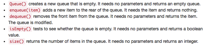
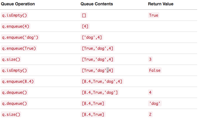
"A queue is an ordered collection of items where the addition of new items happens at one end, called the “rear,” and the removal of existing items occurs at the other end, commonly called the “front.” As an element enters the queue it starts at the rear and makes its way toward the front, waiting until that time when it is the next element to be removed.\n",
"\n",
"The most recently added item in the queue must wait at the end of the collection. The item that has been in the collection the longest is at the front. This ordering principle is sometimes called FIFO, first-in first-out. It is also known as “first-come first-served.”\n",
"\n",
"The simplest example of a queue is the typical line that we all participate in from time to time. We wait in a line for a movie, we wait in the check-out line at a grocery store, and we wait in the cafeteria line (so that we can pop the tray stack)."
]
},
{
"cell_type": "markdown",
"metadata": {},
"source": [
"
"
]
},
{
"cell_type": "code",
"execution_count": 150,
"metadata": {},
"outputs": [],
"source": [
"def dec2bin(number):\n",
" s = myStack()\n",
" while number != 0:\n",
" remainder = number % 2\n",
" s.push(remainder)\n",
" number = number // 2\n",
" binary_string = []\n",
" while not s.isEmpty():\n",
" binary_string.append(str(s.pop()))\n",
" return ''.join(binary_string)"
]
},
{
"cell_type": "code",
"execution_count": 151,
"metadata": {},
"outputs": [
{
"data": {
"text/plain": [
"'1111011'"
]
},
"execution_count": 151,
"metadata": {},
"output_type": "execute_result"
}
],
"source": [
"dec2bin(123)"
]
},
{
"cell_type": "code",
"execution_count": 152,
"metadata": {},
"outputs": [],
"source": [
"def bin2dec(number):\n",
" s = str(number)\n",
" dec = 0\n",
" for i, e in enumerate(s[::-1]):\n",
" dec += int(e) * (2**i)\n",
" return dec"
]
},
{
"cell_type": "code",
"execution_count": 153,
"metadata": {},
"outputs": [
{
"data": {
"text/plain": [
"123"
]
},
"execution_count": 153,
"metadata": {},
"output_type": "execute_result"
}
],
"source": [
"bin2dec(1111011)"
]
},
{
"cell_type": "markdown",
"metadata": {},
"source": [
"## Queues"
]
},
{
"cell_type": "markdown",
"metadata": {},
"source": [
"http://interactivepython.org/runestone/static/pythonds/BasicDS/WhatIsaQueue.html"
]
},
{
"cell_type": "markdown",
"metadata": {},
"source": [
"A queue is an ordered collection of items where the addition of new items happens at one end, called the “rear,” and the removal of existing items occurs at the other end, commonly called the “front.” As an element enters the queue it starts at the rear and makes its way toward the front, waiting until that time when it is the next element to be removed.\n",
"\n",
"The most recently added item in the queue must wait at the end of the collection. The item that has been in the collection the longest is at the front. This ordering principle is sometimes called FIFO, first-in first-out. It is also known as “first-come first-served.”\n",
"\n",
"The simplest example of a queue is the typical line that we all participate in from time to time. We wait in a line for a movie, we wait in the check-out line at a grocery store, and we wait in the cafeteria line (so that we can pop the tray stack)."
]
},
{
"cell_type": "markdown",
"metadata": {},
"source": [
" "
]
},
{
"cell_type": "markdown",
"metadata": {},
"source": [
"**Python implementation**"
]
},
{
"cell_type": "markdown",
"metadata": {},
"source": [
""
]
},
{
"cell_type": "markdown",
"metadata": {},
"source": [
""
]
},
{
"cell_type": "code",
"execution_count": 157,
"metadata": {},
"outputs": [],
"source": [
"class myQueue:\n",
" def __init__(self):\n",
" self.items = []\n",
" self.sz = 0\n",
"\n",
" def enqueue(self, item):\n",
" self.sz += 1\n",
" self.items.append(item)\n",
"\n",
" def dequeue(self):\n",
" if self.sz == 0:\n",
" print(\"Queue is empty\")\n",
" else:\n",
" self.sz -= 1\n",
" return self.items.pop(0)\n",
"\n",
" def size(self):\n",
" return self.sz\n",
"\n",
" def isEmpty(self):\n",
" return self.sz == 0\n",
"\n",
" def __str__(self):\n",
" return str(self.items)"
]
},
{
"cell_type": "code",
"execution_count": 158,
"metadata": {},
"outputs": [],
"source": [
"q = myQueue()"
]
},
{
"cell_type": "code",
"execution_count": 159,
"metadata": {},
"outputs": [],
"source": [
"q.enqueue('hello')"
]
},
{
"cell_type": "code",
"execution_count": 160,
"metadata": {},
"outputs": [],
"source": [
"q.enqueue('dog')"
]
},
{
"cell_type": "code",
"execution_count": 161,
"metadata": {},
"outputs": [],
"source": [
"q.enqueue(3)"
]
},
{
"cell_type": "code",
"execution_count": 162,
"metadata": {
"scrolled": true
},
"outputs": [
{
"data": {
"text/plain": [
"'hello'"
]
},
"execution_count": 162,
"metadata": {},
"output_type": "execute_result"
}
],
"source": [
"q.dequeue()"
]
},
{
"cell_type": "code",
"execution_count": 163,
"metadata": {},
"outputs": [
{
"data": {
"text/plain": [
"'dog'"
]
},
"execution_count": 163,
"metadata": {},
"output_type": "execute_result"
}
],
"source": [
"q.dequeue()"
]
},
{
"cell_type": "code",
"execution_count": 164,
"metadata": {},
"outputs": [
{
"data": {
"text/plain": [
"3"
]
},
"execution_count": 164,
"metadata": {},
"output_type": "execute_result"
}
],
"source": [
"q.dequeue()"
]
},
{
"cell_type": "code",
"execution_count": 165,
"metadata": {},
"outputs": [
{
"data": {
"text/plain": [
"0"
]
},
"execution_count": 165,
"metadata": {},
"output_type": "execute_result"
}
],
"source": [
"q.size()"
]
},
{
"cell_type": "code",
"execution_count": 166,
"metadata": {},
"outputs": [
{
"data": {
"text/plain": [
"True"
]
},
"execution_count": 166,
"metadata": {},
"output_type": "execute_result"
}
],
"source": [
"q.isEmpty()"
]
},
{
"cell_type": "markdown",
"metadata": {},
"source": [
"## Linked Lists"
]
},
{
"cell_type": "markdown",
"metadata": {},
"source": [
"http://interactivepython.org/runestone/static/pythonds/BasicDS/ImplementinganUnorderedListLinkedLists.html"
]
},
{
"cell_type": "markdown",
"metadata": {},
"source": [
"In order to implement an unordered list, we will construct what is commonly known as a linked list. Recall that we need to be sure that we can maintain the relative positioning of the items. However, there is no requirement that we maintain that positioning in contiguous memory."
]
},
{
"cell_type": "markdown",
"metadata": {},
"source": [
"It is important to note that the location of the first item of the list must be explicitly specified. Once we know where the first item is, the first item can tell us where the second is, and so on. The external reference is often referred to as the head of the list. Similarly, the last item needs to know that there is no next item."
]
},
{
"cell_type": "markdown",
"metadata": {},
"source": [
"
"
]
},
{
"cell_type": "markdown",
"metadata": {},
"source": [
"**Python implementation**"
]
},
{
"cell_type": "markdown",
"metadata": {},
"source": [
""
]
},
{
"cell_type": "markdown",
"metadata": {},
"source": [
""
]
},
{
"cell_type": "code",
"execution_count": 157,
"metadata": {},
"outputs": [],
"source": [
"class myQueue:\n",
" def __init__(self):\n",
" self.items = []\n",
" self.sz = 0\n",
"\n",
" def enqueue(self, item):\n",
" self.sz += 1\n",
" self.items.append(item)\n",
"\n",
" def dequeue(self):\n",
" if self.sz == 0:\n",
" print(\"Queue is empty\")\n",
" else:\n",
" self.sz -= 1\n",
" return self.items.pop(0)\n",
"\n",
" def size(self):\n",
" return self.sz\n",
"\n",
" def isEmpty(self):\n",
" return self.sz == 0\n",
"\n",
" def __str__(self):\n",
" return str(self.items)"
]
},
{
"cell_type": "code",
"execution_count": 158,
"metadata": {},
"outputs": [],
"source": [
"q = myQueue()"
]
},
{
"cell_type": "code",
"execution_count": 159,
"metadata": {},
"outputs": [],
"source": [
"q.enqueue('hello')"
]
},
{
"cell_type": "code",
"execution_count": 160,
"metadata": {},
"outputs": [],
"source": [
"q.enqueue('dog')"
]
},
{
"cell_type": "code",
"execution_count": 161,
"metadata": {},
"outputs": [],
"source": [
"q.enqueue(3)"
]
},
{
"cell_type": "code",
"execution_count": 162,
"metadata": {
"scrolled": true
},
"outputs": [
{
"data": {
"text/plain": [
"'hello'"
]
},
"execution_count": 162,
"metadata": {},
"output_type": "execute_result"
}
],
"source": [
"q.dequeue()"
]
},
{
"cell_type": "code",
"execution_count": 163,
"metadata": {},
"outputs": [
{
"data": {
"text/plain": [
"'dog'"
]
},
"execution_count": 163,
"metadata": {},
"output_type": "execute_result"
}
],
"source": [
"q.dequeue()"
]
},
{
"cell_type": "code",
"execution_count": 164,
"metadata": {},
"outputs": [
{
"data": {
"text/plain": [
"3"
]
},
"execution_count": 164,
"metadata": {},
"output_type": "execute_result"
}
],
"source": [
"q.dequeue()"
]
},
{
"cell_type": "code",
"execution_count": 165,
"metadata": {},
"outputs": [
{
"data": {
"text/plain": [
"0"
]
},
"execution_count": 165,
"metadata": {},
"output_type": "execute_result"
}
],
"source": [
"q.size()"
]
},
{
"cell_type": "code",
"execution_count": 166,
"metadata": {},
"outputs": [
{
"data": {
"text/plain": [
"True"
]
},
"execution_count": 166,
"metadata": {},
"output_type": "execute_result"
}
],
"source": [
"q.isEmpty()"
]
},
{
"cell_type": "markdown",
"metadata": {},
"source": [
"## Linked Lists"
]
},
{
"cell_type": "markdown",
"metadata": {},
"source": [
"http://interactivepython.org/runestone/static/pythonds/BasicDS/ImplementinganUnorderedListLinkedLists.html"
]
},
{
"cell_type": "markdown",
"metadata": {},
"source": [
"In order to implement an unordered list, we will construct what is commonly known as a linked list. Recall that we need to be sure that we can maintain the relative positioning of the items. However, there is no requirement that we maintain that positioning in contiguous memory."
]
},
{
"cell_type": "markdown",
"metadata": {},
"source": [
"It is important to note that the location of the first item of the list must be explicitly specified. Once we know where the first item is, the first item can tell us where the second is, and so on. The external reference is often referred to as the head of the list. Similarly, the last item needs to know that there is no next item."
]
},
{
"cell_type": "markdown",
"metadata": {},
"source": [
" "
]
},
{
"cell_type": "markdown",
"metadata": {},
"source": [
"It is important to note that the location of the first item of the list must be explicitly specified. Once we know where the first item is, the first item can tell us where the second is, and so on. The external reference is often referred to as the head of the list. Similarly, the last item needs to know that there is no next item."
]
},
{
"cell_type": "markdown",
"metadata": {},
"source": [
"**Node**"
]
},
{
"cell_type": "markdown",
"metadata": {},
"source": [
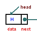
"The basic building block for linked list is node"
]
},
{
"cell_type": "markdown",
"metadata": {},
"source": [
""
]
},
{
"cell_type": "markdown",
"metadata": {},
"source": [
"Each node object must hold at least two pieces of information. First, the node must contain the list item itself. We will call this the data field of the node. In addition, each node must hold a reference to the next node."
]
},
{
"cell_type": "code",
"execution_count": 173,
"metadata": {},
"outputs": [],
"source": [
"class Node:\n",
" def __init__(self, value):\n",
" self.value = value\n",
" self.next = None\n",
"\n",
" def getData(self):\n",
" return self.value\n",
"\n",
" def getNext(self):\n",
" return self.next\n",
"\n",
" def setData(self, newvalue):\n",
" self.value = newvalue\n",
"\n",
" def setNext(self, newnext):\n",
" self.next = newnext"
]
},
{
"cell_type": "code",
"execution_count": 174,
"metadata": {},
"outputs": [],
"source": [
"temp = Node(93)"
]
},
{
"cell_type": "code",
"execution_count": 175,
"metadata": {},
"outputs": [
{
"data": {
"text/plain": [
"93"
]
},
"execution_count": 175,
"metadata": {},
"output_type": "execute_result"
}
],
"source": [
"temp.getData()"
]
},
{
"cell_type": "code",
"execution_count": 176,
"metadata": {},
"outputs": [],
"source": [
"temp.setData(50)"
]
},
{
"cell_type": "code",
"execution_count": 177,
"metadata": {},
"outputs": [
{
"data": {
"text/plain": [
"50"
]
},
"execution_count": 177,
"metadata": {},
"output_type": "execute_result"
}
],
"source": [
"temp.getData()"
]
},
{
"cell_type": "markdown",
"metadata": {},
"source": [
"The special Python reference value None will play an important role in the Node class and later in the linked list itself. A reference to None will denote the fact that there is no next node. Note in the constructor that a node is initially created with next set to None. Since this is sometimes referred to as “grounding the node,” we will use the standard ground symbol to denote a reference that is referring to None. It is always a good idea to explicitly assign None to your initial next reference values."
]
},
{
"cell_type": "markdown",
"metadata": {},
"source": [
"
"
]
},
{
"cell_type": "markdown",
"metadata": {},
"source": [
"It is important to note that the location of the first item of the list must be explicitly specified. Once we know where the first item is, the first item can tell us where the second is, and so on. The external reference is often referred to as the head of the list. Similarly, the last item needs to know that there is no next item."
]
},
{
"cell_type": "markdown",
"metadata": {},
"source": [
"**Node**"
]
},
{
"cell_type": "markdown",
"metadata": {},
"source": [
"The basic building block for linked list is node"
]
},
{
"cell_type": "markdown",
"metadata": {},
"source": [
""
]
},
{
"cell_type": "markdown",
"metadata": {},
"source": [
"Each node object must hold at least two pieces of information. First, the node must contain the list item itself. We will call this the data field of the node. In addition, each node must hold a reference to the next node."
]
},
{
"cell_type": "code",
"execution_count": 173,
"metadata": {},
"outputs": [],
"source": [
"class Node:\n",
" def __init__(self, value):\n",
" self.value = value\n",
" self.next = None\n",
"\n",
" def getData(self):\n",
" return self.value\n",
"\n",
" def getNext(self):\n",
" return self.next\n",
"\n",
" def setData(self, newvalue):\n",
" self.value = newvalue\n",
"\n",
" def setNext(self, newnext):\n",
" self.next = newnext"
]
},
{
"cell_type": "code",
"execution_count": 174,
"metadata": {},
"outputs": [],
"source": [
"temp = Node(93)"
]
},
{
"cell_type": "code",
"execution_count": 175,
"metadata": {},
"outputs": [
{
"data": {
"text/plain": [
"93"
]
},
"execution_count": 175,
"metadata": {},
"output_type": "execute_result"
}
],
"source": [
"temp.getData()"
]
},
{
"cell_type": "code",
"execution_count": 176,
"metadata": {},
"outputs": [],
"source": [
"temp.setData(50)"
]
},
{
"cell_type": "code",
"execution_count": 177,
"metadata": {},
"outputs": [
{
"data": {
"text/plain": [
"50"
]
},
"execution_count": 177,
"metadata": {},
"output_type": "execute_result"
}
],
"source": [
"temp.getData()"
]
},
{
"cell_type": "markdown",
"metadata": {},
"source": [
"The special Python reference value None will play an important role in the Node class and later in the linked list itself. A reference to None will denote the fact that there is no next node. Note in the constructor that a node is initially created with next set to None. Since this is sometimes referred to as “grounding the node,” we will use the standard ground symbol to denote a reference that is referring to None. It is always a good idea to explicitly assign None to your initial next reference values."
]
},
{
"cell_type": "markdown",
"metadata": {},
"source": [
" "
]
},
{
"cell_type": "markdown",
"metadata": {},
"source": [
"**Unordered list (Linkedlist)**"
]
},
{
"cell_type": "markdown",
"metadata": {},
"source": [
"As we suggested above, the unordered list will be built from a collection of nodes, each linked to the next by explicit references. As long as we know where to find the first node (containing the first item), each item after that can be found by successively following the next links. With this in mind, the UnorderedList class must maintain a reference to the first node."
]
},
{
"cell_type": "code",
"execution_count": null,
"metadata": {},
"outputs": [],
"source": [
"class linkedList:\n",
" def __init__(self):\n",
" self.head = None"
]
},
{
"cell_type": "markdown",
"metadata": {},
"source": [
"
"
]
},
{
"cell_type": "markdown",
"metadata": {},
"source": [
"**Unordered list (Linkedlist)**"
]
},
{
"cell_type": "markdown",
"metadata": {},
"source": [
"As we suggested above, the unordered list will be built from a collection of nodes, each linked to the next by explicit references. As long as we know where to find the first node (containing the first item), each item after that can be found by successively following the next links. With this in mind, the UnorderedList class must maintain a reference to the first node."
]
},
{
"cell_type": "code",
"execution_count": null,
"metadata": {},
"outputs": [],
"source": [
"class linkedList:\n",
" def __init__(self):\n",
" self.head = None"
]
},
{
"cell_type": "markdown",
"metadata": {},
"source": [
" "
]
},
{
"cell_type": "markdown",
"metadata": {},
"source": [
"As we discussed in the Node class, the special reference None will again be used to state that the head of the list does not refer to anything."
]
},
{
"cell_type": "code",
"execution_count": 186,
"metadata": {},
"outputs": [],
"source": [
"class linkedList:\n",
" def __init__(self):\n",
" self.head = None\n",
"\n",
" def isEmpty(self):\n",
" return self.head == None"
]
},
{
"cell_type": "code",
"execution_count": 180,
"metadata": {},
"outputs": [],
"source": [
"ll = linkedList()"
]
},
{
"cell_type": "code",
"execution_count": 181,
"metadata": {},
"outputs": [
{
"data": {
"text/plain": [
"True"
]
},
"execution_count": 181,
"metadata": {},
"output_type": "execute_result"
}
],
"source": [
"ll.isEmpty()"
]
},
{
"cell_type": "markdown",
"metadata": {},
"source": [
"The isEmpty method, simply checks to see if the head of the list is a reference to None."
]
},
{
"cell_type": "code",
"execution_count": 183,
"metadata": {},
"outputs": [],
"source": [
"class linkedList:\n",
" def __init__(self):\n",
" self.head = None\n",
"\n",
" def isEmpty(self):\n",
" return self.head == None\n",
"\n",
" def add(self, value):\n",
" if self.isEmpty():\n",
" self.head = Node(value)\n",
" else:\n",
" tmp = Node(value)\n",
" tmp.setNext(self.head)\n",
" self.head = tmp"
]
},
{
"cell_type": "code",
"execution_count": 184,
"metadata": {},
"outputs": [],
"source": [
"mylist = linkedList()\n",
"\n",
"mylist.add(31)\n",
"mylist.add(77)\n",
"mylist.add(17)\n",
"mylist.add(93)\n",
"mylist.add(26)\n",
"mylist.add(54)"
]
},
{
"cell_type": "markdown",
"metadata": {},
"source": [
"
"
]
},
{
"cell_type": "markdown",
"metadata": {},
"source": [
"As we discussed in the Node class, the special reference None will again be used to state that the head of the list does not refer to anything."
]
},
{
"cell_type": "code",
"execution_count": 186,
"metadata": {},
"outputs": [],
"source": [
"class linkedList:\n",
" def __init__(self):\n",
" self.head = None\n",
"\n",
" def isEmpty(self):\n",
" return self.head == None"
]
},
{
"cell_type": "code",
"execution_count": 180,
"metadata": {},
"outputs": [],
"source": [
"ll = linkedList()"
]
},
{
"cell_type": "code",
"execution_count": 181,
"metadata": {},
"outputs": [
{
"data": {
"text/plain": [
"True"
]
},
"execution_count": 181,
"metadata": {},
"output_type": "execute_result"
}
],
"source": [
"ll.isEmpty()"
]
},
{
"cell_type": "markdown",
"metadata": {},
"source": [
"The isEmpty method, simply checks to see if the head of the list is a reference to None."
]
},
{
"cell_type": "code",
"execution_count": 183,
"metadata": {},
"outputs": [],
"source": [
"class linkedList:\n",
" def __init__(self):\n",
" self.head = None\n",
"\n",
" def isEmpty(self):\n",
" return self.head == None\n",
"\n",
" def add(self, value):\n",
" if self.isEmpty():\n",
" self.head = Node(value)\n",
" else:\n",
" tmp = Node(value)\n",
" tmp.setNext(self.head)\n",
" self.head = tmp"
]
},
{
"cell_type": "code",
"execution_count": 184,
"metadata": {},
"outputs": [],
"source": [
"mylist = linkedList()\n",
"\n",
"mylist.add(31)\n",
"mylist.add(77)\n",
"mylist.add(17)\n",
"mylist.add(93)\n",
"mylist.add(26)\n",
"mylist.add(54)"
]
},
{
"cell_type": "markdown",
"metadata": {},
"source": [
" "
]
},
{
"cell_type": "markdown",
"metadata": {},
"source": [
"So, how do we get items into our list? We need to implement the add method. However, before we can do that, we need to address the important question of where in the linked list to place the new item. Since this list is unordered, the specific location of the new item with respect to the other items already in the list is not important. The new item can go anywhere. With that in mind, it makes sense to place the new item in the easiest location possible.\n",
"\n",
"Recall that the linked list structure provides us with only one entry point, the head of the list. All of the other nodes can only be reached by accessing the first node and then following next links. This means that the easiest place to add the new node is right at the head, or beginning, of the list. In other words, we will make the new item the first item of the list and the existing items will need to be linked to this new first item so that they follow."
]
},
{
"cell_type": "markdown",
"metadata": {},
"source": [
"The next methods that we will implement–size, search, and remove–are all based on a technique known as linked list traversal. Traversal refers to the process of systematically visiting each node. To do this we use an external reference that starts at the first node in the list. As we visit each node, we move the reference to the next node by “traversing” the next reference."
]
},
{
"cell_type": "code",
"execution_count": 201,
"metadata": {},
"outputs": [],
"source": [
"class linkedList:\n",
" def __init__(self):\n",
" self.head = None\n",
"\n",
" def isEmpty(self):\n",
" return self.head == None\n",
"\n",
" def add(self, value):\n",
" if self.isEmpty():\n",
" self.head = Node(value)\n",
" else:\n",
" tmp = Node(value)\n",
" tmp.setNext(self.head)\n",
" self.head = tmp\n",
"\n",
" def size(self):\n",
" if self.head == None:\n",
" return 0\n",
"\n",
" counter = 0\n",
" current_node = self.head\n",
" while current_node != None:\n",
" counter += 1\n",
" current_node = current_node.getNext()\n",
" return counter\n",
"\n",
" def search(self, value):\n",
" if self.head == None:\n",
" return \"Empty list\"\n",
"\n",
" current_node = self.head\n",
" found = False\n",
" while found != True and current_node != None:\n",
" if current_node.getData() == value: found = True\n",
" else: current_node = current_node.getNext()\n",
" return found\n",
"\n",
" def remove(self, value):\n",
" if self.head == None: return \"Empty linked list\"\n",
"\n",
" previous_node = None\n",
" current_node = self.head\n",
" found = False\n",
" while current_node != None and found != True:\n",
" if current_node.getData() == value:\n",
" found = True\n",
" else:\n",
" previous_node = current_node\n",
" current_node = current_node.getNext()\n",
" if previous_node == None and found:\n",
" self.head = Node(value)\n",
" else:\n",
" previous_node.setNext(current_node.getNext())"
]
},
{
"cell_type": "markdown",
"metadata": {},
"source": [
"Size"
]
},
{
"cell_type": "markdown",
"metadata": {},
"source": [
"
"
]
},
{
"cell_type": "markdown",
"metadata": {},
"source": [
"So, how do we get items into our list? We need to implement the add method. However, before we can do that, we need to address the important question of where in the linked list to place the new item. Since this list is unordered, the specific location of the new item with respect to the other items already in the list is not important. The new item can go anywhere. With that in mind, it makes sense to place the new item in the easiest location possible.\n",
"\n",
"Recall that the linked list structure provides us with only one entry point, the head of the list. All of the other nodes can only be reached by accessing the first node and then following next links. This means that the easiest place to add the new node is right at the head, or beginning, of the list. In other words, we will make the new item the first item of the list and the existing items will need to be linked to this new first item so that they follow."
]
},
{
"cell_type": "markdown",
"metadata": {},
"source": [
"The next methods that we will implement–size, search, and remove–are all based on a technique known as linked list traversal. Traversal refers to the process of systematically visiting each node. To do this we use an external reference that starts at the first node in the list. As we visit each node, we move the reference to the next node by “traversing” the next reference."
]
},
{
"cell_type": "code",
"execution_count": 201,
"metadata": {},
"outputs": [],
"source": [
"class linkedList:\n",
" def __init__(self):\n",
" self.head = None\n",
"\n",
" def isEmpty(self):\n",
" return self.head == None\n",
"\n",
" def add(self, value):\n",
" if self.isEmpty():\n",
" self.head = Node(value)\n",
" else:\n",
" tmp = Node(value)\n",
" tmp.setNext(self.head)\n",
" self.head = tmp\n",
"\n",
" def size(self):\n",
" if self.head == None:\n",
" return 0\n",
"\n",
" counter = 0\n",
" current_node = self.head\n",
" while current_node != None:\n",
" counter += 1\n",
" current_node = current_node.getNext()\n",
" return counter\n",
"\n",
" def search(self, value):\n",
" if self.head == None:\n",
" return \"Empty list\"\n",
"\n",
" current_node = self.head\n",
" found = False\n",
" while found != True and current_node != None:\n",
" if current_node.getData() == value: found = True\n",
" else: current_node = current_node.getNext()\n",
" return found\n",
"\n",
" def remove(self, value):\n",
" if self.head == None: return \"Empty linked list\"\n",
"\n",
" previous_node = None\n",
" current_node = self.head\n",
" found = False\n",
" while current_node != None and found != True:\n",
" if current_node.getData() == value:\n",
" found = True\n",
" else:\n",
" previous_node = current_node\n",
" current_node = current_node.getNext()\n",
" if previous_node == None and found:\n",
" self.head = Node(value)\n",
" else:\n",
" previous_node.setNext(current_node.getNext())"
]
},
{
"cell_type": "markdown",
"metadata": {},
"source": [
"Size"
]
},
{
"cell_type": "markdown",
"metadata": {},
"source": [
" "
]
},
{
"cell_type": "markdown",
"metadata": {},
"source": [
"Search"
]
},
{
"cell_type": "markdown",
"metadata": {},
"source": [
"
"
]
},
{
"cell_type": "markdown",
"metadata": {},
"source": [
"Search"
]
},
{
"cell_type": "markdown",
"metadata": {},
"source": [
" "
]
},
{
"cell_type": "markdown",
"metadata": {},
"source": [
"Removal"
]
},
{
"cell_type": "markdown",
"metadata": {},
"source": [
"
"
]
},
{
"cell_type": "markdown",
"metadata": {},
"source": [
"Removal"
]
},
{
"cell_type": "markdown",
"metadata": {},
"source": [
" "
]
},
{
"cell_type": "markdown",
"metadata": {},
"source": [
"
"
]
},
{
"cell_type": "markdown",
"metadata": {},
"source": [
" "
]
},
{
"cell_type": "markdown",
"metadata": {},
"source": [
"
"
]
},
{
"cell_type": "markdown",
"metadata": {},
"source": [
" "
]
},
{
"cell_type": "markdown",
"metadata": {},
"source": [
"special case of removal when target of removal is the head itself"
]
},
{
"cell_type": "markdown",
"metadata": {},
"source": [
" "
]
},
{
"cell_type": "markdown",
"metadata": {},
"source": [
"
"
]
},
{
"cell_type": "markdown",
"metadata": {},
"source": [
"special case of removal when target of removal is the head itself"
]
},
{
"cell_type": "markdown",
"metadata": {},
"source": [
" "
]
},
{
"cell_type": "markdown",
"metadata": {},
"source": [
" "
]
},
{
"cell_type": "code",
"execution_count": 202,
"metadata": {},
"outputs": [],
"source": [
"mylist = linkedList()\n",
"\n",
"mylist.add(31)\n",
"mylist.add(77)\n",
"mylist.add(17)\n",
"mylist.add(93)\n",
"mylist.add(26)\n",
"mylist.add(54)"
]
},
{
"cell_type": "code",
"execution_count": 203,
"metadata": {},
"outputs": [
{
"data": {
"text/plain": [
"54"
]
},
"execution_count": 203,
"metadata": {},
"output_type": "execute_result"
}
],
"source": [
"mylist.head.getData()"
]
},
{
"cell_type": "code",
"execution_count": 204,
"metadata": {},
"outputs": [],
"source": [
"mylist.remove(26)"
]
},
{
"cell_type": "code",
"execution_count": 205,
"metadata": {},
"outputs": [
{
"data": {
"text/plain": [
"93"
]
},
"execution_count": 205,
"metadata": {},
"output_type": "execute_result"
}
],
"source": [
"mylist.head.getNext().getData()"
]
},
{
"cell_type": "code",
"execution_count": 206,
"metadata": {},
"outputs": [],
"source": [
"mylist.remove(54)"
]
},
{
"cell_type": "code",
"execution_count": 207,
"metadata": {},
"outputs": [
{
"data": {
"text/plain": [
"54"
]
},
"execution_count": 207,
"metadata": {},
"output_type": "execute_result"
}
],
"source": [
"mylist.head.getData()"
]
},
{
"cell_type": "markdown",
"metadata": {},
"source": [
"Complete linked list"
]
},
{
"cell_type": "code",
"execution_count": 307,
"metadata": {},
"outputs": [],
"source": [
"class linkedList:\n",
" def __init__(self):\n",
" self.head = None\n",
"\n",
" def isEmpty(self):\n",
" return self.head == None\n",
"\n",
" def add(self, value):\n",
" if self.isEmpty():\n",
" self.head = Node(value)\n",
" else:\n",
" tmp = Node(value)\n",
" tmp.setNext(self.head)\n",
" self.head = tmp\n",
"\n",
" def size(self):\n",
" if self.head == None:\n",
" return 0\n",
"\n",
" counter = 0\n",
" current_node = self.head\n",
" while current_node != None:\n",
" counter += 1\n",
" current_node = current_node.getNext()\n",
" return counter\n",
"\n",
" def search(self, value):\n",
" if self.head == None:\n",
" return \"Empty list\"\n",
"\n",
" current_node = self.head\n",
" found = False\n",
" while found != True and current_node != None:\n",
" if current_node.getData() == value: found = True\n",
" else: current_node = current_node.getNext()\n",
" return found\n",
"\n",
" def remove(self, value):\n",
" if self.head == None: return \"Empty linked list\"\n",
"\n",
" previous_node = None\n",
" current_node = self.head\n",
" found = False\n",
" while current_node != None and found != True:\n",
" if current_node.getData() == value:\n",
" found = True\n",
" else:\n",
" previous_node = current_node\n",
" current_node = current_node.getNext()\n",
" if previous_node == None and found:\n",
" self.head = Node(value)\n",
" elif found:\n",
" previous_node.setNext(current_node.getNext())\n",
" else:\n",
" return \"value not in the list\"\n",
"\n",
" def append(self, value):\n",
" if self.head == None:\n",
" self.head = Node(value)\n",
" else:\n",
" current_node = self.head\n",
" while current_node.getNext() != None:\n",
" current_node = current_node.getNext()\n",
" current_node.setNext(Node(value))\n",
"\n",
" def __str__(self):\n",
" if self.head == None:\n",
" return \"Empty list\"\n",
" else:\n",
" current_node = self.head\n",
" l = []\n",
" while current_node != None:\n",
" l.append(current_node.getData())\n",
" current_node = current_node.getNext()\n",
" return str(l)\n",
"\n",
" def sorted_insert(self, value):\n",
" if self.head == None:\n",
" self.head = Node(value)\n",
" else:\n",
" previous = None\n",
" current_node = self.head\n",
" found = False\n",
" while current_node != None and found != True:\n",
" if previous == None:\n",
" if value <= current_node.getData():\n",
" found = True\n",
" else:\n",
" previous = current_node\n",
" current_node = current_node.getNext()\n",
" else:\n",
" if previous.getData() <= value <= current_node.getData():\n",
" found = True\n",
" else:\n",
" previous = current_node\n",
" current_node = current_node.getNext()\n",
"\n",
" if previous == None and found:\n",
" temp = Node(value)\n",
" temp.setNext(self.head)\n",
" self.head = temp\n",
" elif found:\n",
" temp = Node(value)\n",
" temp.setNext(current_node)\n",
" previous.setNext(temp)\n",
" else:\n",
" temp = Node(value)\n",
" previous.setNext(temp)"
]
},
{
"cell_type": "markdown",
"metadata": {},
"source": [
"Questions on linked list"
]
},
{
"cell_type": "markdown",
"metadata": {},
"source": [
"https://www.geeksforgeeks.org/given-a-linked-list-which-is-sorted-how-will-you-insert-in-sorted-way/"
]
},
{
"cell_type": "markdown",
"metadata": {},
"source": [
"Given a sorted linked list and a value to insert, write a function to insert the value in sorted way."
]
},
{
"cell_type": "markdown",
"metadata": {},
"source": [
"See the sorted insert function in the class"
]
},
{
"cell_type": "code",
"execution_count": 308,
"metadata": {},
"outputs": [
{
"name": "stdout",
"output_type": "stream",
"text": [
"[1, 2, 17, 26, 31, 54, 77, 93]\n"
]
}
],
"source": [
"mylist = linkedList()\n",
"mylist.sorted_insert(2)\n",
"mylist.sorted_insert(1)\n",
"mylist.sorted_insert(31)\n",
"mylist.sorted_insert(77)\n",
"mylist.sorted_insert(17)\n",
"mylist.sorted_insert(93)\n",
"mylist.sorted_insert(26)\n",
"mylist.sorted_insert(54)\n",
"\n",
"print(mylist)"
]
},
{
"cell_type": "markdown",
"metadata": {},
"source": [
"https://www.geeksforgeeks.org/compare-two-strings-represented-as-linked-lists/"
]
},
{
"cell_type": "markdown",
"metadata": {},
"source": [
"Compare two strings represented as linked lists"
]
},
{
"cell_type": "markdown",
"metadata": {},
"source": [
"Given two linked lists, represented as linked lists (every character is a node in linked list). Write a function compare() that works similar to strcmp(), i.e., it returns 0 if both strings are same, 1 if first linked list is lexicographically greater, and -1 if second string is lexicographically greater."
]
},
{
"cell_type": "code",
"execution_count": 366,
"metadata": {},
"outputs": [],
"source": [
"def lexcompare(list1, list2):\n",
" c1 = list1.head\n",
" c2 = list2.head\n",
" while c1 != None and c2 != None:\n",
" if c1.getData() == c2.getData():\n",
" c1 = c1.getNext()\n",
" c2 = c2.getNext()\n",
" continue\n",
" elif c1.getData() < c2.getData():\n",
" return 1\n",
" elif c1.getData() > c2.getData():\n",
" return -1\n",
" if c1 == None and c2 == None:\n",
" return 0\n",
" elif c2 == None:\n",
" return 1\n",
" else:\n",
" return -1"
]
},
{
"cell_type": "code",
"execution_count": 367,
"metadata": {},
"outputs": [],
"source": [
"list1 = linkedList()\n",
"list2 = linkedList()\n",
"list1.add('a')\n",
"list1.add('b')\n",
"list1.add('c')\n",
"list1.add('d')"
]
},
{
"cell_type": "code",
"execution_count": 368,
"metadata": {},
"outputs": [],
"source": [
"list2.add('a')\n",
"list2.add('b')\n",
"list2.add('c')\n",
"list2.add('d')"
]
},
{
"cell_type": "code",
"execution_count": 369,
"metadata": {},
"outputs": [
{
"name": "stdout",
"output_type": "stream",
"text": [
"['d', 'c', 'b', 'a']\n"
]
}
],
"source": [
"print(list1)"
]
},
{
"cell_type": "code",
"execution_count": 370,
"metadata": {},
"outputs": [
{
"name": "stdout",
"output_type": "stream",
"text": [
"['d', 'c', 'b', 'a']\n"
]
}
],
"source": [
"print(list2)"
]
},
{
"cell_type": "code",
"execution_count": 371,
"metadata": {},
"outputs": [
{
"data": {
"text/plain": [
"0"
]
},
"execution_count": 371,
"metadata": {},
"output_type": "execute_result"
}
],
"source": [
"lexcompare(list1, list2)"
]
},
{
"cell_type": "markdown",
"metadata": {},
"source": [
"## Tree"
]
},
{
"cell_type": "markdown",
"metadata": {},
"source": [
"Trees are used in many areas of computer science, including operating systems, graphics, database systems, and computer networking. Tree data structures have many things in common with their botanical cousins. A tree data structure has a root, branches, and leaves. The difference between a tree in nature and a tree in computer science is that a tree data structure has its root at the top and its leaves on the bottom."
]
},
{
"cell_type": "markdown",
"metadata": {},
"source": [
"
"
]
},
{
"cell_type": "code",
"execution_count": 202,
"metadata": {},
"outputs": [],
"source": [
"mylist = linkedList()\n",
"\n",
"mylist.add(31)\n",
"mylist.add(77)\n",
"mylist.add(17)\n",
"mylist.add(93)\n",
"mylist.add(26)\n",
"mylist.add(54)"
]
},
{
"cell_type": "code",
"execution_count": 203,
"metadata": {},
"outputs": [
{
"data": {
"text/plain": [
"54"
]
},
"execution_count": 203,
"metadata": {},
"output_type": "execute_result"
}
],
"source": [
"mylist.head.getData()"
]
},
{
"cell_type": "code",
"execution_count": 204,
"metadata": {},
"outputs": [],
"source": [
"mylist.remove(26)"
]
},
{
"cell_type": "code",
"execution_count": 205,
"metadata": {},
"outputs": [
{
"data": {
"text/plain": [
"93"
]
},
"execution_count": 205,
"metadata": {},
"output_type": "execute_result"
}
],
"source": [
"mylist.head.getNext().getData()"
]
},
{
"cell_type": "code",
"execution_count": 206,
"metadata": {},
"outputs": [],
"source": [
"mylist.remove(54)"
]
},
{
"cell_type": "code",
"execution_count": 207,
"metadata": {},
"outputs": [
{
"data": {
"text/plain": [
"54"
]
},
"execution_count": 207,
"metadata": {},
"output_type": "execute_result"
}
],
"source": [
"mylist.head.getData()"
]
},
{
"cell_type": "markdown",
"metadata": {},
"source": [
"Complete linked list"
]
},
{
"cell_type": "code",
"execution_count": 307,
"metadata": {},
"outputs": [],
"source": [
"class linkedList:\n",
" def __init__(self):\n",
" self.head = None\n",
"\n",
" def isEmpty(self):\n",
" return self.head == None\n",
"\n",
" def add(self, value):\n",
" if self.isEmpty():\n",
" self.head = Node(value)\n",
" else:\n",
" tmp = Node(value)\n",
" tmp.setNext(self.head)\n",
" self.head = tmp\n",
"\n",
" def size(self):\n",
" if self.head == None:\n",
" return 0\n",
"\n",
" counter = 0\n",
" current_node = self.head\n",
" while current_node != None:\n",
" counter += 1\n",
" current_node = current_node.getNext()\n",
" return counter\n",
"\n",
" def search(self, value):\n",
" if self.head == None:\n",
" return \"Empty list\"\n",
"\n",
" current_node = self.head\n",
" found = False\n",
" while found != True and current_node != None:\n",
" if current_node.getData() == value: found = True\n",
" else: current_node = current_node.getNext()\n",
" return found\n",
"\n",
" def remove(self, value):\n",
" if self.head == None: return \"Empty linked list\"\n",
"\n",
" previous_node = None\n",
" current_node = self.head\n",
" found = False\n",
" while current_node != None and found != True:\n",
" if current_node.getData() == value:\n",
" found = True\n",
" else:\n",
" previous_node = current_node\n",
" current_node = current_node.getNext()\n",
" if previous_node == None and found:\n",
" self.head = Node(value)\n",
" elif found:\n",
" previous_node.setNext(current_node.getNext())\n",
" else:\n",
" return \"value not in the list\"\n",
"\n",
" def append(self, value):\n",
" if self.head == None:\n",
" self.head = Node(value)\n",
" else:\n",
" current_node = self.head\n",
" while current_node.getNext() != None:\n",
" current_node = current_node.getNext()\n",
" current_node.setNext(Node(value))\n",
"\n",
" def __str__(self):\n",
" if self.head == None:\n",
" return \"Empty list\"\n",
" else:\n",
" current_node = self.head\n",
" l = []\n",
" while current_node != None:\n",
" l.append(current_node.getData())\n",
" current_node = current_node.getNext()\n",
" return str(l)\n",
"\n",
" def sorted_insert(self, value):\n",
" if self.head == None:\n",
" self.head = Node(value)\n",
" else:\n",
" previous = None\n",
" current_node = self.head\n",
" found = False\n",
" while current_node != None and found != True:\n",
" if previous == None:\n",
" if value <= current_node.getData():\n",
" found = True\n",
" else:\n",
" previous = current_node\n",
" current_node = current_node.getNext()\n",
" else:\n",
" if previous.getData() <= value <= current_node.getData():\n",
" found = True\n",
" else:\n",
" previous = current_node\n",
" current_node = current_node.getNext()\n",
"\n",
" if previous == None and found:\n",
" temp = Node(value)\n",
" temp.setNext(self.head)\n",
" self.head = temp\n",
" elif found:\n",
" temp = Node(value)\n",
" temp.setNext(current_node)\n",
" previous.setNext(temp)\n",
" else:\n",
" temp = Node(value)\n",
" previous.setNext(temp)"
]
},
{
"cell_type": "markdown",
"metadata": {},
"source": [
"Questions on linked list"
]
},
{
"cell_type": "markdown",
"metadata": {},
"source": [
"https://www.geeksforgeeks.org/given-a-linked-list-which-is-sorted-how-will-you-insert-in-sorted-way/"
]
},
{
"cell_type": "markdown",
"metadata": {},
"source": [
"Given a sorted linked list and a value to insert, write a function to insert the value in sorted way."
]
},
{
"cell_type": "markdown",
"metadata": {},
"source": [
"See the sorted insert function in the class"
]
},
{
"cell_type": "code",
"execution_count": 308,
"metadata": {},
"outputs": [
{
"name": "stdout",
"output_type": "stream",
"text": [
"[1, 2, 17, 26, 31, 54, 77, 93]\n"
]
}
],
"source": [
"mylist = linkedList()\n",
"mylist.sorted_insert(2)\n",
"mylist.sorted_insert(1)\n",
"mylist.sorted_insert(31)\n",
"mylist.sorted_insert(77)\n",
"mylist.sorted_insert(17)\n",
"mylist.sorted_insert(93)\n",
"mylist.sorted_insert(26)\n",
"mylist.sorted_insert(54)\n",
"\n",
"print(mylist)"
]
},
{
"cell_type": "markdown",
"metadata": {},
"source": [
"https://www.geeksforgeeks.org/compare-two-strings-represented-as-linked-lists/"
]
},
{
"cell_type": "markdown",
"metadata": {},
"source": [
"Compare two strings represented as linked lists"
]
},
{
"cell_type": "markdown",
"metadata": {},
"source": [
"Given two linked lists, represented as linked lists (every character is a node in linked list). Write a function compare() that works similar to strcmp(), i.e., it returns 0 if both strings are same, 1 if first linked list is lexicographically greater, and -1 if second string is lexicographically greater."
]
},
{
"cell_type": "code",
"execution_count": 366,
"metadata": {},
"outputs": [],
"source": [
"def lexcompare(list1, list2):\n",
" c1 = list1.head\n",
" c2 = list2.head\n",
" while c1 != None and c2 != None:\n",
" if c1.getData() == c2.getData():\n",
" c1 = c1.getNext()\n",
" c2 = c2.getNext()\n",
" continue\n",
" elif c1.getData() < c2.getData():\n",
" return 1\n",
" elif c1.getData() > c2.getData():\n",
" return -1\n",
" if c1 == None and c2 == None:\n",
" return 0\n",
" elif c2 == None:\n",
" return 1\n",
" else:\n",
" return -1"
]
},
{
"cell_type": "code",
"execution_count": 367,
"metadata": {},
"outputs": [],
"source": [
"list1 = linkedList()\n",
"list2 = linkedList()\n",
"list1.add('a')\n",
"list1.add('b')\n",
"list1.add('c')\n",
"list1.add('d')"
]
},
{
"cell_type": "code",
"execution_count": 368,
"metadata": {},
"outputs": [],
"source": [
"list2.add('a')\n",
"list2.add('b')\n",
"list2.add('c')\n",
"list2.add('d')"
]
},
{
"cell_type": "code",
"execution_count": 369,
"metadata": {},
"outputs": [
{
"name": "stdout",
"output_type": "stream",
"text": [
"['d', 'c', 'b', 'a']\n"
]
}
],
"source": [
"print(list1)"
]
},
{
"cell_type": "code",
"execution_count": 370,
"metadata": {},
"outputs": [
{
"name": "stdout",
"output_type": "stream",
"text": [
"['d', 'c', 'b', 'a']\n"
]
}
],
"source": [
"print(list2)"
]
},
{
"cell_type": "code",
"execution_count": 371,
"metadata": {},
"outputs": [
{
"data": {
"text/plain": [
"0"
]
},
"execution_count": 371,
"metadata": {},
"output_type": "execute_result"
}
],
"source": [
"lexcompare(list1, list2)"
]
},
{
"cell_type": "markdown",
"metadata": {},
"source": [
"## Tree"
]
},
{
"cell_type": "markdown",
"metadata": {},
"source": [
"Trees are used in many areas of computer science, including operating systems, graphics, database systems, and computer networking. Tree data structures have many things in common with their botanical cousins. A tree data structure has a root, branches, and leaves. The difference between a tree in nature and a tree in computer science is that a tree data structure has its root at the top and its leaves on the bottom."
]
},
{
"cell_type": "markdown",
"metadata": {},
"source": [
" "
]
},
{
"cell_type": "markdown",
"metadata": {},
"source": [
"http://interactivepython.org/runestone/static/pythonds/Trees/VocabularyandDefinitions.html"
]
},
{
"cell_type": "markdown",
"metadata": {},
"source": [
"**Terminology**"
]
},
{
"cell_type": "markdown",
"metadata": {},
"source": [
"* Node:\n",
"A node is a fundamental part of a tree. It can have a name, which we call the “key.” A node may also have additional information. We call this additional information the “payload.” While the payload information is not central to many tree algorithms, it is often critical in applications that make use of trees.\n",
"* Edge:\n",
"An edge is another fundamental part of a tree. An edge connects two nodes to show that there is a relationship between them. Every node (except the root) is connected by exactly one incoming edge from another node. Each node may have several outgoing edges.\n",
"* Root:\n",
"The root of the tree is the only node in the tree that has no incoming edges. In Figure Figure 2, / is the root of the tree.\n",
"* Path:\n",
"A path is an ordered list of nodes that are connected by edges. For example, Mammal → Carnivora → Felidae → Felis → Domestica is a path.\n",
"* Children:\n",
"The set of nodes c that have incoming edges from the same node to are said to be the children of that node. In Figure Figure 2, nodes log/, spool/, and yp/ are the children of node var/.\n",
"* Parent:\n",
"A node is the parent of all the nodes it connects to with outgoing edges. In Figure 2 the node var/ is the parent of nodes log/, spool/, and yp/.\n",
"* Sibling:\n",
"Nodes in the tree that are children of the same parent are said to be siblings. The nodes etc/ and usr/ are siblings in the filesystem tree.\n",
"* Subtree:\n",
"A subtree is a set of nodes and edges comprised of a parent and all the descendants of that parent.\n",
"* Leaf Node:\n",
"A leaf node is a node that has no children. For example, Human and Chimpanzee are leaf nodes in Figure 1.\n",
"* Level:\n",
"The level of a node n is the number of edges on the path from the root node to n. For example, the level of the Felis node in Figure 1 is five. By definition, the level of the root node is zero.\n",
"* Height:\n",
"The height of a tree is equal to the maximum level of any node in the tree. The height of the tree in Figure 2 is two."
]
},
{
"cell_type": "markdown",
"metadata": {},
"source": [
"Point of view 1: List of list"
]
},
{
"cell_type": "markdown",
"metadata": {},
"source": [
"
"
]
},
{
"cell_type": "markdown",
"metadata": {},
"source": [
"http://interactivepython.org/runestone/static/pythonds/Trees/VocabularyandDefinitions.html"
]
},
{
"cell_type": "markdown",
"metadata": {},
"source": [
"**Terminology**"
]
},
{
"cell_type": "markdown",
"metadata": {},
"source": [
"* Node:\n",
"A node is a fundamental part of a tree. It can have a name, which we call the “key.” A node may also have additional information. We call this additional information the “payload.” While the payload information is not central to many tree algorithms, it is often critical in applications that make use of trees.\n",
"* Edge:\n",
"An edge is another fundamental part of a tree. An edge connects two nodes to show that there is a relationship between them. Every node (except the root) is connected by exactly one incoming edge from another node. Each node may have several outgoing edges.\n",
"* Root:\n",
"The root of the tree is the only node in the tree that has no incoming edges. In Figure Figure 2, / is the root of the tree.\n",
"* Path:\n",
"A path is an ordered list of nodes that are connected by edges. For example, Mammal → Carnivora → Felidae → Felis → Domestica is a path.\n",
"* Children:\n",
"The set of nodes c that have incoming edges from the same node to are said to be the children of that node. In Figure Figure 2, nodes log/, spool/, and yp/ are the children of node var/.\n",
"* Parent:\n",
"A node is the parent of all the nodes it connects to with outgoing edges. In Figure 2 the node var/ is the parent of nodes log/, spool/, and yp/.\n",
"* Sibling:\n",
"Nodes in the tree that are children of the same parent are said to be siblings. The nodes etc/ and usr/ are siblings in the filesystem tree.\n",
"* Subtree:\n",
"A subtree is a set of nodes and edges comprised of a parent and all the descendants of that parent.\n",
"* Leaf Node:\n",
"A leaf node is a node that has no children. For example, Human and Chimpanzee are leaf nodes in Figure 1.\n",
"* Level:\n",
"The level of a node n is the number of edges on the path from the root node to n. For example, the level of the Felis node in Figure 1 is five. By definition, the level of the root node is zero.\n",
"* Height:\n",
"The height of a tree is equal to the maximum level of any node in the tree. The height of the tree in Figure 2 is two."
]
},
{
"cell_type": "markdown",
"metadata": {},
"source": [
"Point of view 1: List of list"
]
},
{
"cell_type": "markdown",
"metadata": {},
"source": [
" "
]
},
{
"cell_type": "markdown",
"metadata": {},
"source": [
"Point of view 2: Subtree recursive"
]
},
{
"cell_type": "markdown",
"metadata": {},
"source": [
"
"
]
},
{
"cell_type": "markdown",
"metadata": {},
"source": [
"Point of view 2: Subtree recursive"
]
},
{
"cell_type": "markdown",
"metadata": {},
"source": [
" "
]
},
{
"cell_type": "markdown",
"metadata": {},
"source": [
"### Binary Tree"
]
},
{
"cell_type": "markdown",
"metadata": {},
"source": [
"Tree where every node has 2 childs at max"
]
},
{
"cell_type": "markdown",
"metadata": {},
"source": [
"**Using list of lists**"
]
},
{
"cell_type": "markdown",
"metadata": {},
"source": [
"I won't explain the list of lists approach as it's not that useful"
]
},
{
"cell_type": "code",
"execution_count": 372,
"metadata": {},
"outputs": [],
"source": [
"def BinaryTree(r):\n",
" return [r, [], []]\n",
"\n",
"\n",
"def insertLeft(root, newBranch):\n",
" t = root.pop(1)\n",
" if len(t) > 1:\n",
" root.insert(1, [newBranch, t, []])\n",
" else:\n",
" root.insert(1, [newBranch, [], []])\n",
" return root\n",
"\n",
"\n",
"def insertRight(root, newBranch):\n",
" t = root.pop(2)\n",
" if len(t) > 1:\n",
" root.insert(2, [newBranch, [], t])\n",
" else:\n",
" root.insert(2, [newBranch, [], []])\n",
" return root\n",
"\n",
"\n",
"def getRootVal(root):\n",
" return root[0]\n",
"\n",
"\n",
"def setRootVal(root, newVal):\n",
" root[0] = newVal\n",
"\n",
"\n",
"def getLeftChild(root):\n",
" return root[1]\n",
"\n",
"\n",
"def getRightChild(root):\n",
" return root[2]"
]
},
{
"cell_type": "code",
"execution_count": 373,
"metadata": {},
"outputs": [
{
"name": "stdout",
"output_type": "stream",
"text": [
"[5, [4, [], []], []]\n",
"[3, [9, [4, [], []], []], [7, [], [6, [], []]]]\n",
"[3, [9, [11, [4, [], []], []], []], [7, [], [6, [], []]]]\n",
"[6, [], []]\n"
]
}
],
"source": [
"r = BinaryTree(3)\n",
"insertLeft(r, 4)\n",
"insertLeft(r, 5)\n",
"insertRight(r, 6)\n",
"insertRight(r, 7)\n",
"l = getLeftChild(r)\n",
"print(l)\n",
"\n",
"setRootVal(l, 9)\n",
"print(r)\n",
"insertLeft(l, 11)\n",
"print(r)\n",
"print(getRightChild(getRightChild(r)))"
]
},
{
"cell_type": "markdown",
"metadata": {},
"source": [
"**Subtree approach of building binary tree**"
]
},
{
"cell_type": "markdown",
"metadata": {},
"source": [
"In this case we will define a class that has attributes for the root value, as well as the left and right subtrees."
]
},
{
"cell_type": "markdown",
"metadata": {},
"source": [
"
"
]
},
{
"cell_type": "markdown",
"metadata": {},
"source": [
"### Binary Tree"
]
},
{
"cell_type": "markdown",
"metadata": {},
"source": [
"Tree where every node has 2 childs at max"
]
},
{
"cell_type": "markdown",
"metadata": {},
"source": [
"**Using list of lists**"
]
},
{
"cell_type": "markdown",
"metadata": {},
"source": [
"I won't explain the list of lists approach as it's not that useful"
]
},
{
"cell_type": "code",
"execution_count": 372,
"metadata": {},
"outputs": [],
"source": [
"def BinaryTree(r):\n",
" return [r, [], []]\n",
"\n",
"\n",
"def insertLeft(root, newBranch):\n",
" t = root.pop(1)\n",
" if len(t) > 1:\n",
" root.insert(1, [newBranch, t, []])\n",
" else:\n",
" root.insert(1, [newBranch, [], []])\n",
" return root\n",
"\n",
"\n",
"def insertRight(root, newBranch):\n",
" t = root.pop(2)\n",
" if len(t) > 1:\n",
" root.insert(2, [newBranch, [], t])\n",
" else:\n",
" root.insert(2, [newBranch, [], []])\n",
" return root\n",
"\n",
"\n",
"def getRootVal(root):\n",
" return root[0]\n",
"\n",
"\n",
"def setRootVal(root, newVal):\n",
" root[0] = newVal\n",
"\n",
"\n",
"def getLeftChild(root):\n",
" return root[1]\n",
"\n",
"\n",
"def getRightChild(root):\n",
" return root[2]"
]
},
{
"cell_type": "code",
"execution_count": 373,
"metadata": {},
"outputs": [
{
"name": "stdout",
"output_type": "stream",
"text": [
"[5, [4, [], []], []]\n",
"[3, [9, [4, [], []], []], [7, [], [6, [], []]]]\n",
"[3, [9, [11, [4, [], []], []], []], [7, [], [6, [], []]]]\n",
"[6, [], []]\n"
]
}
],
"source": [
"r = BinaryTree(3)\n",
"insertLeft(r, 4)\n",
"insertLeft(r, 5)\n",
"insertRight(r, 6)\n",
"insertRight(r, 7)\n",
"l = getLeftChild(r)\n",
"print(l)\n",
"\n",
"setRootVal(l, 9)\n",
"print(r)\n",
"insertLeft(l, 11)\n",
"print(r)\n",
"print(getRightChild(getRightChild(r)))"
]
},
{
"cell_type": "markdown",
"metadata": {},
"source": [
"**Subtree approach of building binary tree**"
]
},
{
"cell_type": "markdown",
"metadata": {},
"source": [
"In this case we will define a class that has attributes for the root value, as well as the left and right subtrees."
]
},
{
"cell_type": "markdown",
"metadata": {},
"source": [
" "
]
},
{
"cell_type": "markdown",
"metadata": {},
"source": [
"The important thing to remember about this representation is that the attributes left and right will become references to other instances of the BinaryTree class. For example, when we insert a new left child into the tree we create another instance of BinaryTree and modify self.leftChild in the root to reference the new tree."
]
},
{
"cell_type": "markdown",
"metadata": {},
"source": [
"The constructor function expects to get some kind of object to store in the root. Just like you can store any object you like in a list, the root object of a tree can be a reference to any object. For our early examples, we will store the name of the node as the root value."
]
},
{
"cell_type": "code",
"execution_count": 385,
"metadata": {},
"outputs": [],
"source": [
"class BinaryTree:\n",
" def __init__(self, root):\n",
" self.key = root\n",
" self.left = None\n",
" self.right = None\n",
"\n",
" def insertLeft(self, leftnode):\n",
" if self.left == None:\n",
" self.left = BinaryTree(leftnode)\n",
" else:\n",
" temp = BinaryTree(leftnode)\n",
" temp.left = self.left\n",
" self.left = temp\n",
"\n",
" def insertRight(self, rightnode):\n",
" if self.right == None:\n",
" self.right = BinaryTree(rightnode)\n",
" else:\n",
" temp = BinaryTree(rightnode)\n",
" temp.right = self.right\n",
" self.right = temp\n",
"\n",
" def getRightChild(self):\n",
" return self.right\n",
"\n",
" def getLeftChild(self):\n",
" return self.left\n",
"\n",
" def setRootVal(self, newroot):\n",
" self.key = newroot\n",
"\n",
" def getRootVal(self):\n",
" return self.key\n",
"\n",
" def preorder(self):\n",
" print(self.key)\n",
" if self.left:\n",
" self.left.preorder()\n",
" if self.right:\n",
" self.right.preorder()\n",
"\n",
" def inorder(self):\n",
" if self.left:\n",
" self.left.inorder()\n",
" print(self.key)\n",
" if self.right:\n",
" self.right.inorder()\n",
"\n",
" def postorder(self):\n",
" if self.left:\n",
" self.left.inorder()\n",
" if self.right:\n",
" self.right.inorder()\n",
" print(self.key)"
]
},
{
"cell_type": "markdown",
"metadata": {},
"source": [
"We must consider two cases for insertion. The first case is characterized by a node with no existing left child. When there is no left child, simply add a node to the tree. The second case is characterized by a node with an existing left child. In the second case, we insert a node and push the existing child down one level in the tree. "
]
},
{
"cell_type": "markdown",
"metadata": {},
"source": [
"* preorder:\n",
"In a preorder traversal, we visit the root node first, then recursively do a preorder traversal of the left subtree, followed by a recursive preorder traversal of the right subtree.\n",
"* inorder:\n",
"In an inorder traversal, we recursively do an inorder traversal on the left subtree, visit the root node, and finally do a recursive inorder traversal of the right subtree.\n",
"* postorder:\n",
"In a postorder traversal, we recursively do a postorder traversal of the left subtree and the right subtree followed by a visit to the root node."
]
},
{
"cell_type": "code",
"execution_count": 517,
"metadata": {},
"outputs": [],
"source": [
"r = BinaryTree('a')\n",
"r.insertLeft('b')\n",
"r.insertRight('c')\n",
"r.insertLeft('d')\n",
"r.insertRight('e')"
]
},
{
"cell_type": "code",
"execution_count": 518,
"metadata": {},
"outputs": [
{
"name": "stdout",
"output_type": "stream",
"text": [
"a\n",
"d\n",
"b\n",
"e\n",
"c\n"
]
}
],
"source": [
"r.preorder()"
]
},
{
"cell_type": "code",
"execution_count": 519,
"metadata": {},
"outputs": [
{
"name": "stdout",
"output_type": "stream",
"text": [
"b\n",
"d\n",
"a\n",
"e\n",
"c\n"
]
}
],
"source": [
"r.inorder()"
]
},
{
"cell_type": "code",
"execution_count": 520,
"metadata": {},
"outputs": [
{
"name": "stdout",
"output_type": "stream",
"text": [
"b\n",
"d\n",
"e\n",
"c\n",
"a\n"
]
}
],
"source": [
"r.postorder()"
]
},
{
"cell_type": "markdown",
"metadata": {},
"source": [
"### Binary search tree"
]
},
{
"cell_type": "markdown",
"metadata": {},
"source": [
"A binary search tree relies on the property that **keys that are less than the parent are found in the left subtree, and keys that are greater than the parent are found in the right subtree**. We will call this the bst property."
]
},
{
"cell_type": "markdown",
"metadata": {},
"source": [
"
"
]
},
{
"cell_type": "markdown",
"metadata": {},
"source": [
"The important thing to remember about this representation is that the attributes left and right will become references to other instances of the BinaryTree class. For example, when we insert a new left child into the tree we create another instance of BinaryTree and modify self.leftChild in the root to reference the new tree."
]
},
{
"cell_type": "markdown",
"metadata": {},
"source": [
"The constructor function expects to get some kind of object to store in the root. Just like you can store any object you like in a list, the root object of a tree can be a reference to any object. For our early examples, we will store the name of the node as the root value."
]
},
{
"cell_type": "code",
"execution_count": 385,
"metadata": {},
"outputs": [],
"source": [
"class BinaryTree:\n",
" def __init__(self, root):\n",
" self.key = root\n",
" self.left = None\n",
" self.right = None\n",
"\n",
" def insertLeft(self, leftnode):\n",
" if self.left == None:\n",
" self.left = BinaryTree(leftnode)\n",
" else:\n",
" temp = BinaryTree(leftnode)\n",
" temp.left = self.left\n",
" self.left = temp\n",
"\n",
" def insertRight(self, rightnode):\n",
" if self.right == None:\n",
" self.right = BinaryTree(rightnode)\n",
" else:\n",
" temp = BinaryTree(rightnode)\n",
" temp.right = self.right\n",
" self.right = temp\n",
"\n",
" def getRightChild(self):\n",
" return self.right\n",
"\n",
" def getLeftChild(self):\n",
" return self.left\n",
"\n",
" def setRootVal(self, newroot):\n",
" self.key = newroot\n",
"\n",
" def getRootVal(self):\n",
" return self.key\n",
"\n",
" def preorder(self):\n",
" print(self.key)\n",
" if self.left:\n",
" self.left.preorder()\n",
" if self.right:\n",
" self.right.preorder()\n",
"\n",
" def inorder(self):\n",
" if self.left:\n",
" self.left.inorder()\n",
" print(self.key)\n",
" if self.right:\n",
" self.right.inorder()\n",
"\n",
" def postorder(self):\n",
" if self.left:\n",
" self.left.inorder()\n",
" if self.right:\n",
" self.right.inorder()\n",
" print(self.key)"
]
},
{
"cell_type": "markdown",
"metadata": {},
"source": [
"We must consider two cases for insertion. The first case is characterized by a node with no existing left child. When there is no left child, simply add a node to the tree. The second case is characterized by a node with an existing left child. In the second case, we insert a node and push the existing child down one level in the tree. "
]
},
{
"cell_type": "markdown",
"metadata": {},
"source": [
"* preorder:\n",
"In a preorder traversal, we visit the root node first, then recursively do a preorder traversal of the left subtree, followed by a recursive preorder traversal of the right subtree.\n",
"* inorder:\n",
"In an inorder traversal, we recursively do an inorder traversal on the left subtree, visit the root node, and finally do a recursive inorder traversal of the right subtree.\n",
"* postorder:\n",
"In a postorder traversal, we recursively do a postorder traversal of the left subtree and the right subtree followed by a visit to the root node."
]
},
{
"cell_type": "code",
"execution_count": 517,
"metadata": {},
"outputs": [],
"source": [
"r = BinaryTree('a')\n",
"r.insertLeft('b')\n",
"r.insertRight('c')\n",
"r.insertLeft('d')\n",
"r.insertRight('e')"
]
},
{
"cell_type": "code",
"execution_count": 518,
"metadata": {},
"outputs": [
{
"name": "stdout",
"output_type": "stream",
"text": [
"a\n",
"d\n",
"b\n",
"e\n",
"c\n"
]
}
],
"source": [
"r.preorder()"
]
},
{
"cell_type": "code",
"execution_count": 519,
"metadata": {},
"outputs": [
{
"name": "stdout",
"output_type": "stream",
"text": [
"b\n",
"d\n",
"a\n",
"e\n",
"c\n"
]
}
],
"source": [
"r.inorder()"
]
},
{
"cell_type": "code",
"execution_count": 520,
"metadata": {},
"outputs": [
{
"name": "stdout",
"output_type": "stream",
"text": [
"b\n",
"d\n",
"e\n",
"c\n",
"a\n"
]
}
],
"source": [
"r.postorder()"
]
},
{
"cell_type": "markdown",
"metadata": {},
"source": [
"### Binary search tree"
]
},
{
"cell_type": "markdown",
"metadata": {},
"source": [
"A binary search tree relies on the property that **keys that are less than the parent are found in the left subtree, and keys that are greater than the parent are found in the right subtree**. We will call this the bst property."
]
},
{
"cell_type": "markdown",
"metadata": {},
"source": [
" "
]
},
{
"cell_type": "markdown",
"metadata": {},
"source": [
"Implementation uses two classes:\n",
"* bst — can operate on a tree even if it’s empty\n",
"* bstnode — does most of the work"
]
},
{
"cell_type": "code",
"execution_count": 393,
"metadata": {},
"outputs": [],
"source": [
"class bstnode:\n",
" def __init__(self, key, val):\n",
" self.key = key\n",
" self.val = val\n",
" self.left = None\n",
" self.right = None\n",
"\n",
" def getVal(self):\n",
" return self.val\n",
"\n",
" def setVal(self, newval):\n",
" self.val = newval"
]
},
{
"cell_type": "code",
"execution_count": 514,
"metadata": {},
"outputs": [],
"source": [
"class bst:\n",
" def __init__(self):\n",
" self.root = None\n",
"\n",
" def insert(self, key, val):\n",
" if self.root == None:\n",
" self.root = bstnode(key, val)\n",
" else:\n",
" self.insert_node(self.root, key, val)\n",
"\n",
" def insert_node(self, root, key, val):\n",
" if key < root.key:\n",
" if root.left is None:\n",
" root.left = bstnode(key, val)\n",
" else:\n",
" insert_node(root.left, key, val)\n",
" elif key > root.key:\n",
" if root.right is None:\n",
" root.right = bstnode(key, val)\n",
" else:\n",
" root.setVal(val)\n",
"\n",
" def find(self, searchkey):\n",
" return self.find_node(self.root, searchkey)\n",
"\n",
" def find_node(self, root, searchkey):\n",
" if root is None: return \"Empty tree\"\n",
" elif searchkey == root.key:\n",
" return root.val\n",
" elif searchkey < root.key:\n",
" return self.find_node(root.left, searchkey)\n",
" else:\n",
" return self.find_node(root.right, searchkey)\n",
"\n",
" def traverse(self, type='preorder'):\n",
" if self.root:\n",
" if type == 'preorder':\n",
" return self.preorder(self.root)\n",
" elif type == 'inorder':\n",
" return self.inorder(self.root)\n",
" else:\n",
" return self.postorder(self.root)\n",
" else:\n",
" return \"Empty Tree\""
]
},
{
"cell_type": "markdown",
"metadata": {},
"source": [
"Inserting a node"
]
},
{
"cell_type": "markdown",
"metadata": {},
"source": [
"
"
]
},
{
"cell_type": "markdown",
"metadata": {},
"source": [
"Implementation uses two classes:\n",
"* bst — can operate on a tree even if it’s empty\n",
"* bstnode — does most of the work"
]
},
{
"cell_type": "code",
"execution_count": 393,
"metadata": {},
"outputs": [],
"source": [
"class bstnode:\n",
" def __init__(self, key, val):\n",
" self.key = key\n",
" self.val = val\n",
" self.left = None\n",
" self.right = None\n",
"\n",
" def getVal(self):\n",
" return self.val\n",
"\n",
" def setVal(self, newval):\n",
" self.val = newval"
]
},
{
"cell_type": "code",
"execution_count": 514,
"metadata": {},
"outputs": [],
"source": [
"class bst:\n",
" def __init__(self):\n",
" self.root = None\n",
"\n",
" def insert(self, key, val):\n",
" if self.root == None:\n",
" self.root = bstnode(key, val)\n",
" else:\n",
" self.insert_node(self.root, key, val)\n",
"\n",
" def insert_node(self, root, key, val):\n",
" if key < root.key:\n",
" if root.left is None:\n",
" root.left = bstnode(key, val)\n",
" else:\n",
" insert_node(root.left, key, val)\n",
" elif key > root.key:\n",
" if root.right is None:\n",
" root.right = bstnode(key, val)\n",
" else:\n",
" root.setVal(val)\n",
"\n",
" def find(self, searchkey):\n",
" return self.find_node(self.root, searchkey)\n",
"\n",
" def find_node(self, root, searchkey):\n",
" if root is None: return \"Empty tree\"\n",
" elif searchkey == root.key:\n",
" return root.val\n",
" elif searchkey < root.key:\n",
" return self.find_node(root.left, searchkey)\n",
" else:\n",
" return self.find_node(root.right, searchkey)\n",
"\n",
" def traverse(self, type='preorder'):\n",
" if self.root:\n",
" if type == 'preorder':\n",
" return self.preorder(self.root)\n",
" elif type == 'inorder':\n",
" return self.inorder(self.root)\n",
" else:\n",
" return self.postorder(self.root)\n",
" else:\n",
" return \"Empty Tree\""
]
},
{
"cell_type": "markdown",
"metadata": {},
"source": [
"Inserting a node"
]
},
{
"cell_type": "markdown",
"metadata": {},
"source": [
" "
]
},
{
"cell_type": "code",
"execution_count": 515,
"metadata": {},
"outputs": [],
"source": [
"mybst = bst()\n",
"\n",
"mybst.insert(100, \"Jon\")\n",
"\n",
"mybst.insert(120, \"Ron\")\n",
"\n",
"mybst.insert(90, \"Don\")"
]
},
{
"cell_type": "markdown",
"metadata": {},
"source": [
"## Graphs"
]
},
{
"cell_type": "markdown",
"metadata": {},
"source": [
"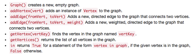"
]
},
{
"cell_type": "markdown",
"metadata": {},
"source": [
"**Adjacency matrix**"
]
},
{
"cell_type": "markdown",
"metadata": {},
"source": [
"
"
]
},
{
"cell_type": "code",
"execution_count": 515,
"metadata": {},
"outputs": [],
"source": [
"mybst = bst()\n",
"\n",
"mybst.insert(100, \"Jon\")\n",
"\n",
"mybst.insert(120, \"Ron\")\n",
"\n",
"mybst.insert(90, \"Don\")"
]
},
{
"cell_type": "markdown",
"metadata": {},
"source": [
"## Graphs"
]
},
{
"cell_type": "markdown",
"metadata": {},
"source": [
""
]
},
{
"cell_type": "markdown",
"metadata": {},
"source": [
"**Adjacency matrix**"
]
},
{
"cell_type": "markdown",
"metadata": {},
"source": [
" "
]
},
{
"cell_type": "markdown",
"metadata": {},
"source": [
"One of the easiest ways to implement a graph is to use a two-dimensional matrix. In this matrix implementation, each of the rows and columns represent a vertex in the graph. The value that is stored in the cell at the intersection of row v and column w indicates if there is an edge from vertex v to vertex w. When two vertices are connected by an edge, we say that they are adjacent."
]
},
{
"cell_type": "markdown",
"metadata": {},
"source": [
"However, notice that most of the cells in the matrix are empty. Because most of the cells are empty we say that this matrix is “sparse.”"
]
},
{
"cell_type": "markdown",
"metadata": {},
"source": [
"**Adjacency List**"
]
},
{
"cell_type": "markdown",
"metadata": {},
"source": [
"
"
]
},
{
"cell_type": "markdown",
"metadata": {},
"source": [
"One of the easiest ways to implement a graph is to use a two-dimensional matrix. In this matrix implementation, each of the rows and columns represent a vertex in the graph. The value that is stored in the cell at the intersection of row v and column w indicates if there is an edge from vertex v to vertex w. When two vertices are connected by an edge, we say that they are adjacent."
]
},
{
"cell_type": "markdown",
"metadata": {},
"source": [
"However, notice that most of the cells in the matrix are empty. Because most of the cells are empty we say that this matrix is “sparse.”"
]
},
{
"cell_type": "markdown",
"metadata": {},
"source": [
"**Adjacency List**"
]
},
{
"cell_type": "markdown",
"metadata": {},
"source": [
" "
]
},
{
"cell_type": "markdown",
"metadata": {},
"source": [
"**Implementation**"
]
},
{
"cell_type": "markdown",
"metadata": {},
"source": [
"Using dictionaries, it is easy to implement the adjacency list in Python. In our implementation of the Graph abstract data type we will create two classes, `Graph`, which holds the master list of vertices, and `Vertex`, which will represent each vertex in the graph."
]
},
{
"cell_type": "markdown",
"metadata": {},
"source": [
"**Vertex**"
]
},
{
"cell_type": "markdown",
"metadata": {},
"source": [
"Each Vertex uses a dictionary to keep track of the vertices to which it is connected, and the weight of each edge. This dictionary is called connectedTo. The listing below shows the code for the Vertex class. The constructor simply initializes the id, which will typically be a string, and the connectedTo dictionary. The addNeighbor method is used add a connection from this vertex to another. The getConnections method returns all of the vertices in the adjacency list, as represented by the connectedTo instance variable. The getWeight method returns the weight of the edge from this vertex to the vertex passed as a parameter."
]
},
{
"cell_type": "code",
"execution_count": 423,
"metadata": {},
"outputs": [],
"source": [
"class vertex:\n",
" def __init__(self, key):\n",
" self.key = key\n",
" self.connections = {}\n",
"\n",
" def getKey(self):\n",
" return self.key\n",
"\n",
" def getneighbors(self):\n",
" return self.connections.keys()\n",
"\n",
" def addneighbors(self, key, weight=1):\n",
" self.connections[key] = weight\n",
"\n",
" def getedge(self, key):\n",
" return self.connections[key]\n",
"\n",
" def setedge(self, key, newweight):\n",
" self.connections[key] = newweight\n",
"\n",
" def __str__(self):\n",
" return f\"Connected to the following vertices:{str([v for v in self.connections])}\""
]
},
{
"cell_type": "code",
"execution_count": 424,
"metadata": {},
"outputs": [],
"source": [
"v = vertex('shikhar')"
]
},
{
"cell_type": "code",
"execution_count": 425,
"metadata": {},
"outputs": [],
"source": [
"v.addneighbors('prince', 100)"
]
},
{
"cell_type": "code",
"execution_count": 426,
"metadata": {},
"outputs": [
{
"name": "stdout",
"output_type": "stream",
"text": [
"Connected to the following vertices:['prince']\n"
]
}
],
"source": [
"print(v)"
]
},
{
"cell_type": "code",
"execution_count": 427,
"metadata": {},
"outputs": [
{
"data": {
"text/plain": [
"dict_keys(['prince'])"
]
},
"execution_count": 427,
"metadata": {},
"output_type": "execute_result"
}
],
"source": [
"v.getneighbors()"
]
},
{
"cell_type": "code",
"execution_count": 428,
"metadata": {},
"outputs": [
{
"data": {
"text/plain": [
"'shikhar'"
]
},
"execution_count": 428,
"metadata": {},
"output_type": "execute_result"
}
],
"source": [
"v.getKey()"
]
},
{
"cell_type": "code",
"execution_count": 430,
"metadata": {},
"outputs": [
{
"data": {
"text/plain": [
"100"
]
},
"execution_count": 430,
"metadata": {},
"output_type": "execute_result"
}
],
"source": [
"v.getedge('prince')"
]
},
{
"cell_type": "markdown",
"metadata": {},
"source": [
"**Graph**"
]
},
{
"cell_type": "markdown",
"metadata": {},
"source": [
"The Graph class, shown in the next listing, contains a dictionary that maps vertex names to vertex objects. In Figure, this dictionary object is represented by the shaded gray box. Graph also provides methods for adding vertices to a graph and connecting one vertex to another. The getVertices method returns the names of all of the vertices in the graph. In addition, we have implemented the __iter__ method to make it easy to iterate over all the vertex objects in a particular graph. Together, the two methods allow you to iterate over the vertices in a graph by name, or by the objects themselves."
]
},
{
"cell_type": "code",
"execution_count": 453,
"metadata": {},
"outputs": [],
"source": [
"class Graph:\n",
" def __init__(self):\n",
" self.vertexlist = {}\n",
" self.numVertices = 0\n",
"\n",
" def addvertex(self, key):\n",
" self.numVertices += 1\n",
" v = vertex(key)\n",
" self.vertexlist[key] = v\n",
"\n",
" def getvertex(self, key):\n",
" if key in vertexlist:\n",
" return vertexlist[key]\n",
" else:\n",
" return \"Not found\"\n",
"\n",
" def __contains__(self, key):\n",
" return key in self.vertexlist.keys()\n",
"\n",
" def addedge(self, key1, key2, weight=1):\n",
" if key1 not in self.vertexlist:\n",
" v = vertex(key1)\n",
" self.vertexlist[key1] = v\n",
" if key2 not in self.vertexlist:\n",
" v = vertex(key2)\n",
" self.vertexlist[key2] = v\n",
" self.vertexlist[key1].addneighbors(key2, weight)\n",
"\n",
" def getvertices(self):\n",
" return self.vertexlist.keys()\n",
"\n",
" def __iter__(self):\n",
" return iter(self.vertexlist.values())"
]
},
{
"cell_type": "code",
"execution_count": 553,
"metadata": {},
"outputs": [],
"source": [
"g = Graph()\n",
"\n",
"g.addvertex('shikhar')\n",
"\n",
"g.addvertex('prince')\n",
"\n",
"g.addvertex('kerem')\n",
"\n",
"g.addedge('shikhar', 'kerem', 100)\n",
"\n",
"g.addedge('shikhar', 'prince', 200)\n",
"\n",
"g.addedge('shikhar', 'ronaldo', 200)\n",
"\n",
"g.addedge('kerem', 'prince', 300)\n",
"\n",
"g.addedge('kerem', 'neerja', 500)\n",
"\n",
"g.addedge('neerja', 'akshay', 600)\n",
"\n",
"g.addedge('kerem', 'messi', 600)"
]
},
{
"cell_type": "code",
"execution_count": 564,
"metadata": {},
"outputs": [
{
"data": {
"text/plain": [
"dict_keys(['shikhar', 'prince', 'kerem', 'ronaldo', 'neerja', 'akshay', 'messi'])"
]
},
"execution_count": 564,
"metadata": {},
"output_type": "execute_result"
}
],
"source": [
"g.getvertices()"
]
},
{
"cell_type": "code",
"execution_count": 565,
"metadata": {},
"outputs": [
{
"data": {
"text/plain": [
"True"
]
},
"execution_count": 565,
"metadata": {},
"output_type": "execute_result"
}
],
"source": [
"'shikhar' in g"
]
},
{
"cell_type": "code",
"execution_count": 566,
"metadata": {},
"outputs": [
{
"data": {
"text/plain": [
"False"
]
},
"execution_count": 566,
"metadata": {},
"output_type": "execute_result"
}
],
"source": [
"'Jon' in g"
]
},
{
"cell_type": "markdown",
"metadata": {},
"source": [
"### Graph traversal"
]
},
{
"cell_type": "markdown",
"metadata": {},
"source": [
"
"
]
},
{
"cell_type": "markdown",
"metadata": {},
"source": [
"**Implementation**"
]
},
{
"cell_type": "markdown",
"metadata": {},
"source": [
"Using dictionaries, it is easy to implement the adjacency list in Python. In our implementation of the Graph abstract data type we will create two classes, `Graph`, which holds the master list of vertices, and `Vertex`, which will represent each vertex in the graph."
]
},
{
"cell_type": "markdown",
"metadata": {},
"source": [
"**Vertex**"
]
},
{
"cell_type": "markdown",
"metadata": {},
"source": [
"Each Vertex uses a dictionary to keep track of the vertices to which it is connected, and the weight of each edge. This dictionary is called connectedTo. The listing below shows the code for the Vertex class. The constructor simply initializes the id, which will typically be a string, and the connectedTo dictionary. The addNeighbor method is used add a connection from this vertex to another. The getConnections method returns all of the vertices in the adjacency list, as represented by the connectedTo instance variable. The getWeight method returns the weight of the edge from this vertex to the vertex passed as a parameter."
]
},
{
"cell_type": "code",
"execution_count": 423,
"metadata": {},
"outputs": [],
"source": [
"class vertex:\n",
" def __init__(self, key):\n",
" self.key = key\n",
" self.connections = {}\n",
"\n",
" def getKey(self):\n",
" return self.key\n",
"\n",
" def getneighbors(self):\n",
" return self.connections.keys()\n",
"\n",
" def addneighbors(self, key, weight=1):\n",
" self.connections[key] = weight\n",
"\n",
" def getedge(self, key):\n",
" return self.connections[key]\n",
"\n",
" def setedge(self, key, newweight):\n",
" self.connections[key] = newweight\n",
"\n",
" def __str__(self):\n",
" return f\"Connected to the following vertices:{str([v for v in self.connections])}\""
]
},
{
"cell_type": "code",
"execution_count": 424,
"metadata": {},
"outputs": [],
"source": [
"v = vertex('shikhar')"
]
},
{
"cell_type": "code",
"execution_count": 425,
"metadata": {},
"outputs": [],
"source": [
"v.addneighbors('prince', 100)"
]
},
{
"cell_type": "code",
"execution_count": 426,
"metadata": {},
"outputs": [
{
"name": "stdout",
"output_type": "stream",
"text": [
"Connected to the following vertices:['prince']\n"
]
}
],
"source": [
"print(v)"
]
},
{
"cell_type": "code",
"execution_count": 427,
"metadata": {},
"outputs": [
{
"data": {
"text/plain": [
"dict_keys(['prince'])"
]
},
"execution_count": 427,
"metadata": {},
"output_type": "execute_result"
}
],
"source": [
"v.getneighbors()"
]
},
{
"cell_type": "code",
"execution_count": 428,
"metadata": {},
"outputs": [
{
"data": {
"text/plain": [
"'shikhar'"
]
},
"execution_count": 428,
"metadata": {},
"output_type": "execute_result"
}
],
"source": [
"v.getKey()"
]
},
{
"cell_type": "code",
"execution_count": 430,
"metadata": {},
"outputs": [
{
"data": {
"text/plain": [
"100"
]
},
"execution_count": 430,
"metadata": {},
"output_type": "execute_result"
}
],
"source": [
"v.getedge('prince')"
]
},
{
"cell_type": "markdown",
"metadata": {},
"source": [
"**Graph**"
]
},
{
"cell_type": "markdown",
"metadata": {},
"source": [
"The Graph class, shown in the next listing, contains a dictionary that maps vertex names to vertex objects. In Figure, this dictionary object is represented by the shaded gray box. Graph also provides methods for adding vertices to a graph and connecting one vertex to another. The getVertices method returns the names of all of the vertices in the graph. In addition, we have implemented the __iter__ method to make it easy to iterate over all the vertex objects in a particular graph. Together, the two methods allow you to iterate over the vertices in a graph by name, or by the objects themselves."
]
},
{
"cell_type": "code",
"execution_count": 453,
"metadata": {},
"outputs": [],
"source": [
"class Graph:\n",
" def __init__(self):\n",
" self.vertexlist = {}\n",
" self.numVertices = 0\n",
"\n",
" def addvertex(self, key):\n",
" self.numVertices += 1\n",
" v = vertex(key)\n",
" self.vertexlist[key] = v\n",
"\n",
" def getvertex(self, key):\n",
" if key in vertexlist:\n",
" return vertexlist[key]\n",
" else:\n",
" return \"Not found\"\n",
"\n",
" def __contains__(self, key):\n",
" return key in self.vertexlist.keys()\n",
"\n",
" def addedge(self, key1, key2, weight=1):\n",
" if key1 not in self.vertexlist:\n",
" v = vertex(key1)\n",
" self.vertexlist[key1] = v\n",
" if key2 not in self.vertexlist:\n",
" v = vertex(key2)\n",
" self.vertexlist[key2] = v\n",
" self.vertexlist[key1].addneighbors(key2, weight)\n",
"\n",
" def getvertices(self):\n",
" return self.vertexlist.keys()\n",
"\n",
" def __iter__(self):\n",
" return iter(self.vertexlist.values())"
]
},
{
"cell_type": "code",
"execution_count": 553,
"metadata": {},
"outputs": [],
"source": [
"g = Graph()\n",
"\n",
"g.addvertex('shikhar')\n",
"\n",
"g.addvertex('prince')\n",
"\n",
"g.addvertex('kerem')\n",
"\n",
"g.addedge('shikhar', 'kerem', 100)\n",
"\n",
"g.addedge('shikhar', 'prince', 200)\n",
"\n",
"g.addedge('shikhar', 'ronaldo', 200)\n",
"\n",
"g.addedge('kerem', 'prince', 300)\n",
"\n",
"g.addedge('kerem', 'neerja', 500)\n",
"\n",
"g.addedge('neerja', 'akshay', 600)\n",
"\n",
"g.addedge('kerem', 'messi', 600)"
]
},
{
"cell_type": "code",
"execution_count": 564,
"metadata": {},
"outputs": [
{
"data": {
"text/plain": [
"dict_keys(['shikhar', 'prince', 'kerem', 'ronaldo', 'neerja', 'akshay', 'messi'])"
]
},
"execution_count": 564,
"metadata": {},
"output_type": "execute_result"
}
],
"source": [
"g.getvertices()"
]
},
{
"cell_type": "code",
"execution_count": 565,
"metadata": {},
"outputs": [
{
"data": {
"text/plain": [
"True"
]
},
"execution_count": 565,
"metadata": {},
"output_type": "execute_result"
}
],
"source": [
"'shikhar' in g"
]
},
{
"cell_type": "code",
"execution_count": 566,
"metadata": {},
"outputs": [
{
"data": {
"text/plain": [
"False"
]
},
"execution_count": 566,
"metadata": {},
"output_type": "execute_result"
}
],
"source": [
"'Jon' in g"
]
},
{
"cell_type": "markdown",
"metadata": {},
"source": [
"### Graph traversal"
]
},
{
"cell_type": "markdown",
"metadata": {},
"source": [
" "
]
},
{
"cell_type": "markdown",
"metadata": {},
"source": [
"
"
]
},
{
"cell_type": "markdown",
"metadata": {},
"source": [
" "
]
},
{
"cell_type": "markdown",
"metadata": {},
"source": [
"Source: https://medium.com/basecs/breaking-down-breadth-first-search-cebe696709d9"
]
},
{
"cell_type": "markdown",
"metadata": {},
"source": [
"**Breadth first search**"
]
},
{
"cell_type": "markdown",
"metadata": {},
"source": [
"*A unique thing about BFS is that it lends itself quite nicely to determining the shortest path between any node in the graph and the “parent” node*"
]
},
{
"cell_type": "markdown",
"metadata": {},
"source": [
"https://medium.com/basecs/going-broad-in-a-graph-bfs-traversal-959bd1a09255"
]
},
{
"cell_type": "markdown",
"metadata": {},
"source": [
"The backbone of a breadth-first graph traversal consists of these basic steps:\n",
"\n",
"* Add a node/vertex from the graph to a queue of nodes to be “visited”.\n",
"* Visit the topmost node in the queue, and mark it as such.\n",
"* If that node has any neighbors, check to see if they have been “visited” or not.\n",
"* Add any neighboring nodes that still need to be “visited” to the queue.\n",
"* Remove the node we’ve visited from the queue."
]
},
{
"cell_type": "code",
"execution_count": 569,
"metadata": {},
"outputs": [],
"source": [
"def bfs(graph, start_vertex):\n",
" visited = {v: False for v in graph.getvertices()}\n",
"\n",
" queue = []\n",
"\n",
" queue.append(start_vertex)\n",
"\n",
" visited[start_vertex] = True\n",
"\n",
" while queue:\n",
"\n",
" current = queue.pop(0)\n",
" print(current)\n",
" current_nn = graph.vertexlist[current].getneighbors()\n",
"\n",
" for v in current_nn:\n",
" if visited[v] == False:\n",
" queue.append(v)\n",
" visited[v] = True"
]
},
{
"cell_type": "code",
"execution_count": 553,
"metadata": {},
"outputs": [],
"source": [
"g = Graph()\n",
"\n",
"g.addvertex('shikhar')\n",
"\n",
"g.addvertex('prince')\n",
"\n",
"g.addvertex('kerem')\n",
"\n",
"g.addedge('shikhar', 'kerem', 100)\n",
"\n",
"g.addedge('shikhar', 'prince', 200)\n",
"\n",
"g.addedge('shikhar', 'ronaldo', 200)\n",
"\n",
"g.addedge('kerem', 'prince', 300)\n",
"\n",
"g.addedge('kerem', 'neerja', 500)\n",
"\n",
"g.addedge('neerja', 'akshay', 600)\n",
"\n",
"g.addedge('kerem', 'messi', 600)"
]
},
{
"cell_type": "code",
"execution_count": 570,
"metadata": {},
"outputs": [
{
"name": "stdout",
"output_type": "stream",
"text": [
"shikhar\n",
"kerem\n",
"prince\n",
"ronaldo\n",
"neerja\n",
"messi\n",
"akshay\n"
]
}
],
"source": [
"bfs(g, 'shikhar')"
]
},
{
"cell_type": "markdown",
"metadata": {},
"source": [
"**Depth first search**"
]
},
{
"cell_type": "markdown",
"metadata": {},
"source": [
"*The depth-first search algorithm allows us to determine whether two nodes, node x and node y, have a path between them. The DFS algorithm does this by looking at all of the children of the starting node, node x, until it reaches node y. It does this by recursively taking the same steps, again and again, in order to determine if such a path between two nodes even exists.*"
]
},
{
"cell_type": "code",
"execution_count": 575,
"metadata": {},
"outputs": [],
"source": [
"def dfs(graph, start_vertex, visited=[]):\n",
" if start_vertex not in visited:\n",
" visited.append(start_vertex)\n",
" print(start_vertex)\n",
" current = graph.vertexlist[start_vertex]\n",
" for v in current.getneighbors():\n",
" dfs(graph, v, visited)"
]
},
{
"cell_type": "code",
"execution_count": 576,
"metadata": {},
"outputs": [],
"source": [
"g = Graph()\n",
"\n",
"g.addvertex('shikhar')\n",
"\n",
"g.addvertex('prince')\n",
"\n",
"g.addvertex('kerem')\n",
"\n",
"g.addedge('shikhar', 'kerem', 100)\n",
"\n",
"g.addedge('shikhar', 'prince', 200)\n",
"\n",
"g.addedge('shikhar', 'ronaldo', 200)\n",
"\n",
"g.addedge('kerem', 'prince', 300)\n",
"\n",
"g.addedge('kerem', 'neerja', 500)\n",
"\n",
"g.addedge('neerja', 'akshay', 600)\n",
"\n",
"g.addedge('kerem', 'messi', 600)"
]
},
{
"cell_type": "code",
"execution_count": 577,
"metadata": {},
"outputs": [
{
"name": "stdout",
"output_type": "stream",
"text": [
"shikhar\n",
"kerem\n",
"prince\n",
"neerja\n",
"akshay\n",
"messi\n",
"ronaldo\n"
]
}
],
"source": [
"dfs(g, 'shikhar')"
]
},
{
"cell_type": "markdown",
"metadata": {},
"source": [
"# Future additions"
]
},
{
"cell_type": "markdown",
"metadata": {},
"source": [
"* Graph shortest path\n",
"* Existence of path\n",
"* Connected components\n",
"* Traversal for binary search tree"
]
},
{
"cell_type": "markdown",
"metadata": {},
"source": [
"# References and useful links:"
]
},
{
"cell_type": "markdown",
"metadata": {},
"source": [
"* Visualization of these concepst : https://visualgo.net/en\n",
"* Detailed discussion on datastructures: https://medium.com/basecs"
]
},
{
"cell_type": "code",
"execution_count": null,
"metadata": {},
"outputs": [],
"source": []
}
],
"metadata": {
"kernelspec": {
"display_name": "Python 3",
"language": "python",
"name": "python3"
},
"language_info": {
"codemirror_mode": {
"name": "ipython",
"version": 3
},
"file_extension": ".py",
"mimetype": "text/x-python",
"name": "python",
"nbconvert_exporter": "python",
"pygments_lexer": "ipython3",
"version": "3.6.5"
},
"toc": {
"nav_menu": {},
"number_sections": true,
"sideBar": true,
"skip_h1_title": false,
"toc_cell": true,
"toc_position": {},
"toc_section_display": "none",
"toc_window_display": false
}
},
"nbformat": 4,
"nbformat_minor": 2
}
"
]
},
{
"cell_type": "markdown",
"metadata": {},
"source": [
"Source: https://medium.com/basecs/breaking-down-breadth-first-search-cebe696709d9"
]
},
{
"cell_type": "markdown",
"metadata": {},
"source": [
"**Breadth first search**"
]
},
{
"cell_type": "markdown",
"metadata": {},
"source": [
"*A unique thing about BFS is that it lends itself quite nicely to determining the shortest path between any node in the graph and the “parent” node*"
]
},
{
"cell_type": "markdown",
"metadata": {},
"source": [
"https://medium.com/basecs/going-broad-in-a-graph-bfs-traversal-959bd1a09255"
]
},
{
"cell_type": "markdown",
"metadata": {},
"source": [
"The backbone of a breadth-first graph traversal consists of these basic steps:\n",
"\n",
"* Add a node/vertex from the graph to a queue of nodes to be “visited”.\n",
"* Visit the topmost node in the queue, and mark it as such.\n",
"* If that node has any neighbors, check to see if they have been “visited” or not.\n",
"* Add any neighboring nodes that still need to be “visited” to the queue.\n",
"* Remove the node we’ve visited from the queue."
]
},
{
"cell_type": "code",
"execution_count": 569,
"metadata": {},
"outputs": [],
"source": [
"def bfs(graph, start_vertex):\n",
" visited = {v: False for v in graph.getvertices()}\n",
"\n",
" queue = []\n",
"\n",
" queue.append(start_vertex)\n",
"\n",
" visited[start_vertex] = True\n",
"\n",
" while queue:\n",
"\n",
" current = queue.pop(0)\n",
" print(current)\n",
" current_nn = graph.vertexlist[current].getneighbors()\n",
"\n",
" for v in current_nn:\n",
" if visited[v] == False:\n",
" queue.append(v)\n",
" visited[v] = True"
]
},
{
"cell_type": "code",
"execution_count": 553,
"metadata": {},
"outputs": [],
"source": [
"g = Graph()\n",
"\n",
"g.addvertex('shikhar')\n",
"\n",
"g.addvertex('prince')\n",
"\n",
"g.addvertex('kerem')\n",
"\n",
"g.addedge('shikhar', 'kerem', 100)\n",
"\n",
"g.addedge('shikhar', 'prince', 200)\n",
"\n",
"g.addedge('shikhar', 'ronaldo', 200)\n",
"\n",
"g.addedge('kerem', 'prince', 300)\n",
"\n",
"g.addedge('kerem', 'neerja', 500)\n",
"\n",
"g.addedge('neerja', 'akshay', 600)\n",
"\n",
"g.addedge('kerem', 'messi', 600)"
]
},
{
"cell_type": "code",
"execution_count": 570,
"metadata": {},
"outputs": [
{
"name": "stdout",
"output_type": "stream",
"text": [
"shikhar\n",
"kerem\n",
"prince\n",
"ronaldo\n",
"neerja\n",
"messi\n",
"akshay\n"
]
}
],
"source": [
"bfs(g, 'shikhar')"
]
},
{
"cell_type": "markdown",
"metadata": {},
"source": [
"**Depth first search**"
]
},
{
"cell_type": "markdown",
"metadata": {},
"source": [
"*The depth-first search algorithm allows us to determine whether two nodes, node x and node y, have a path between them. The DFS algorithm does this by looking at all of the children of the starting node, node x, until it reaches node y. It does this by recursively taking the same steps, again and again, in order to determine if such a path between two nodes even exists.*"
]
},
{
"cell_type": "code",
"execution_count": 575,
"metadata": {},
"outputs": [],
"source": [
"def dfs(graph, start_vertex, visited=[]):\n",
" if start_vertex not in visited:\n",
" visited.append(start_vertex)\n",
" print(start_vertex)\n",
" current = graph.vertexlist[start_vertex]\n",
" for v in current.getneighbors():\n",
" dfs(graph, v, visited)"
]
},
{
"cell_type": "code",
"execution_count": 576,
"metadata": {},
"outputs": [],
"source": [
"g = Graph()\n",
"\n",
"g.addvertex('shikhar')\n",
"\n",
"g.addvertex('prince')\n",
"\n",
"g.addvertex('kerem')\n",
"\n",
"g.addedge('shikhar', 'kerem', 100)\n",
"\n",
"g.addedge('shikhar', 'prince', 200)\n",
"\n",
"g.addedge('shikhar', 'ronaldo', 200)\n",
"\n",
"g.addedge('kerem', 'prince', 300)\n",
"\n",
"g.addedge('kerem', 'neerja', 500)\n",
"\n",
"g.addedge('neerja', 'akshay', 600)\n",
"\n",
"g.addedge('kerem', 'messi', 600)"
]
},
{
"cell_type": "code",
"execution_count": 577,
"metadata": {},
"outputs": [
{
"name": "stdout",
"output_type": "stream",
"text": [
"shikhar\n",
"kerem\n",
"prince\n",
"neerja\n",
"akshay\n",
"messi\n",
"ronaldo\n"
]
}
],
"source": [
"dfs(g, 'shikhar')"
]
},
{
"cell_type": "markdown",
"metadata": {},
"source": [
"# Future additions"
]
},
{
"cell_type": "markdown",
"metadata": {},
"source": [
"* Graph shortest path\n",
"* Existence of path\n",
"* Connected components\n",
"* Traversal for binary search tree"
]
},
{
"cell_type": "markdown",
"metadata": {},
"source": [
"# References and useful links:"
]
},
{
"cell_type": "markdown",
"metadata": {},
"source": [
"* Visualization of these concepst : https://visualgo.net/en\n",
"* Detailed discussion on datastructures: https://medium.com/basecs"
]
},
{
"cell_type": "code",
"execution_count": null,
"metadata": {},
"outputs": [],
"source": []
}
],
"metadata": {
"kernelspec": {
"display_name": "Python 3",
"language": "python",
"name": "python3"
},
"language_info": {
"codemirror_mode": {
"name": "ipython",
"version": 3
},
"file_extension": ".py",
"mimetype": "text/x-python",
"name": "python",
"nbconvert_exporter": "python",
"pygments_lexer": "ipython3",
"version": "3.6.5"
},
"toc": {
"nav_menu": {},
"number_sections": true,
"sideBar": true,
"skip_h1_title": false,
"toc_cell": true,
"toc_position": {},
"toc_section_display": "none",
"toc_window_display": false
}
},
"nbformat": 4,
"nbformat_minor": 2
}