
All about orthogonal polynomials.
[](https://pypi.org/project/orthopy) [](https://pypi.org/pypi/orthopy/) [](https://github.com/nschloe/orthopy) [](https://pepy.tech/project/orthopy) [](https://discord.gg/hnTJ5MRX2Y) [](https://github.com/nschloe/orthopy) orthopy provides various orthogonal polynomial classes for [lines](#line-segment--1-1-with-weight-function-1-x%CE%B1-1-x%CE%B2), [triangles](#triangle-42), [disks](#disk-s2), [spheres](#sphere-u2), [n-cubes](#n-cube-cn), [the *n*D space with weight function exp(-r2)](#nd-space-with-weight-function-exp-r2-enr2) and more. All computations are done using numerically stable recurrence schemes. Furthermore, all functions are fully vectorized and can return results in _exact arithmetic_. ### Installation Install orthopy [from PyPI](https://pypi.org/project/orthopy/) with ``` pip install orthopy ``` ### How to get a license Licenses for personal and academic use can be purchased [here](https://buy.stripe.com/aEUg1H38OgDw5qMfZ3). You'll receive a confirmation email with a license key. Install the key with ``` plm add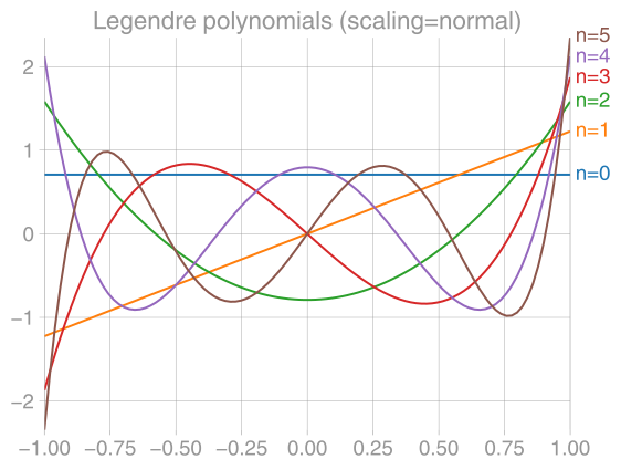 |
|  |
|  |
| :---------------------------------------------------------------------------------------------: | :-----------------------------------------------------------------------------------------------: | :-----------------------------------------------------------------------------------------------: |
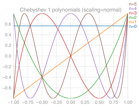
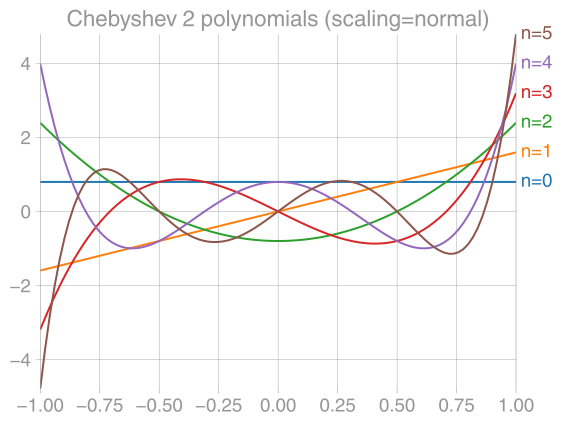
| Legendre | Chebyshev 1 | Chebyshev 2 |
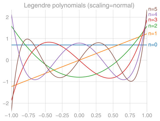
Jacobi, Gegenbauer (α=β), Chebyshev 1 (α=β=-1/2), Chebyshev 2 (α=β=1/2), Legendre
(α=β=0) polynomials.
```python
import orthopy
orthopy.c1.legendre.Eval(x, "normal")
orthopy.c1.chebyshev1.Eval(x, "normal")
orthopy.c1.chebyshev2.Eval(x, "normal")
orthopy.c1.gegenbauer.Eval(x, "normal", lmbda)
orthopy.c1.jacobi.Eval(x, "normal", alpha, beta)
```
The plots above are generated with
```python
import orthopy
orthopy.c1.jacobi.show(5, "normal", 0.0, 0.0)
# plot, savefig also exist
```
Recurrence coefficients can be explicitly retrieved by
```python
import orthopy
rc = orthopy.c1.jacobi.RecurrenceCoefficients(
"monic", # or "classical", "normal"
alpha=0, beta=0, symbolic=True
)
print(rc.p0)
for k in range(5):
print(rc[k])
```
```
1
(1, 0, None)
(1, 0, 1/3)
(1, 0, 4/15)
(1, 0, 9/35)
(1, 0, 16/63)
```
### 1D half-space with weight function xα exp(-r)
|
| :---------------------------------------------------------------------------------------------: | :-----------------------------------------------------------------------------------------------: | :-----------------------------------------------------------------------------------------------: |
| Legendre | Chebyshev 1 | Chebyshev 2 |
Jacobi, Gegenbauer (α=β), Chebyshev 1 (α=β=-1/2), Chebyshev 2 (α=β=1/2), Legendre
(α=β=0) polynomials.
```python
import orthopy
orthopy.c1.legendre.Eval(x, "normal")
orthopy.c1.chebyshev1.Eval(x, "normal")
orthopy.c1.chebyshev2.Eval(x, "normal")
orthopy.c1.gegenbauer.Eval(x, "normal", lmbda)
orthopy.c1.jacobi.Eval(x, "normal", alpha, beta)
```
The plots above are generated with
```python
import orthopy
orthopy.c1.jacobi.show(5, "normal", 0.0, 0.0)
# plot, savefig also exist
```
Recurrence coefficients can be explicitly retrieved by
```python
import orthopy
rc = orthopy.c1.jacobi.RecurrenceCoefficients(
"monic", # or "classical", "normal"
alpha=0, beta=0, symbolic=True
)
print(rc.p0)
for k in range(5):
print(rc[k])
```
```
1
(1, 0, None)
(1, 0, 1/3)
(1, 0, 4/15)
(1, 0, 9/35)
(1, 0, 16/63)
```
### 1D half-space with weight function xα exp(-r)
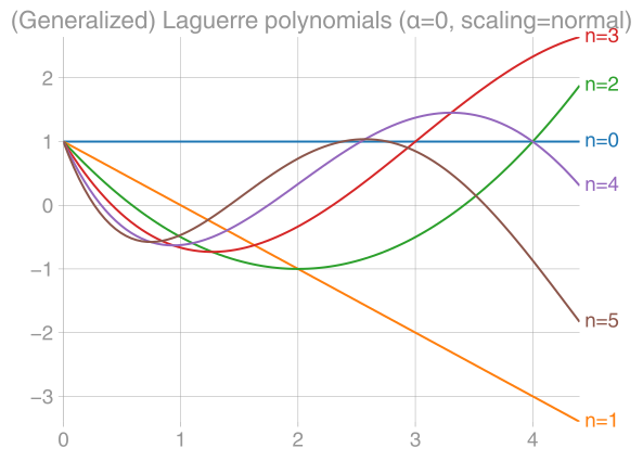 (Generalized) Laguerre polynomials.
```python
evaluator = orthopy.e1r.Eval(x, alpha=0, scaling="normal")
```
### 1D space with weight function exp(-r2)
(Generalized) Laguerre polynomials.
```python
evaluator = orthopy.e1r.Eval(x, alpha=0, scaling="normal")
```
### 1D space with weight function exp(-r2)
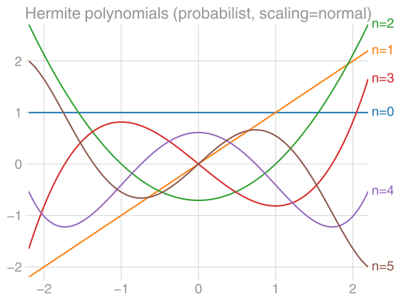 Hermite polynomials come in two standardizations:
- `"physicists"` (against the weight function `exp(-x ** 2)`
- `"probabilists"` (against the weight function `1 / sqrt(2 * pi) * exp(-x ** 2 / 2)`
```python
evaluator = orthopy.e1r2.Eval(
x,
"probabilists", # or "physicists"
"normal"
)
```
#### Associated Legendre "polynomials"
Hermite polynomials come in two standardizations:
- `"physicists"` (against the weight function `exp(-x ** 2)`
- `"probabilists"` (against the weight function `1 / sqrt(2 * pi) * exp(-x ** 2 / 2)`
```python
evaluator = orthopy.e1r2.Eval(
x,
"probabilists", # or "physicists"
"normal"
)
```
#### Associated Legendre "polynomials"
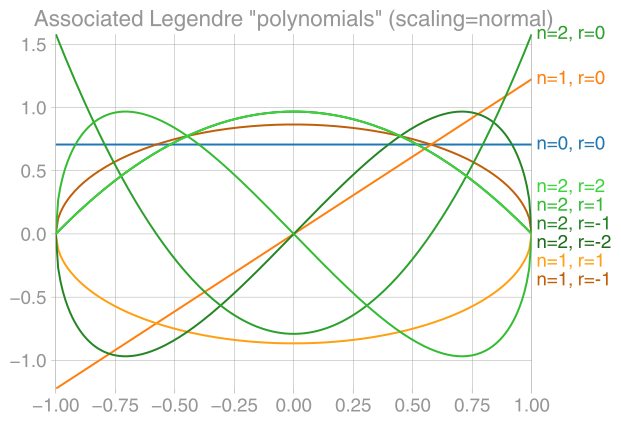 Not all of those are polynomials, so they should really be called associated Legendre
_functions_. The kth iteration contains _2k+1_ functions, indexed from
_-k_ to _k_. (See the color grouping in the above plot.)
```python
evaluator = orthopy.c1.associated_legendre.Eval(
x, phi=None, standardization="natural", with_condon_shortley_phase=True
)
```
### Triangle (_T2_)
Not all of those are polynomials, so they should really be called associated Legendre
_functions_. The kth iteration contains _2k+1_ functions, indexed from
_-k_ to _k_. (See the color grouping in the above plot.)
```python
evaluator = orthopy.c1.associated_legendre.Eval(
x, phi=None, standardization="natural", with_condon_shortley_phase=True
)
```
### Triangle (_T2_)
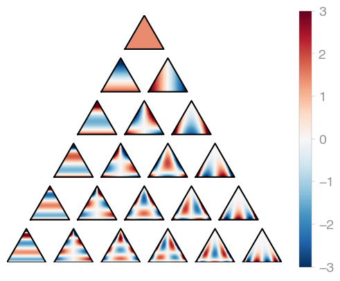 orthopy's triangle orthogonal polynomials are evaluated in terms of [barycentric
coordinates](https://en.wikipedia.org/wiki/Barycentric_coordinate_system), so the
`X.shape[0]` has to be 3.
```python
import orthopy
bary = [0.1, 0.7, 0.2]
evaluator = orthopy.t2.Eval(bary, "normal")
```
### Disk (_S2_)
|
orthopy's triangle orthogonal polynomials are evaluated in terms of [barycentric
coordinates](https://en.wikipedia.org/wiki/Barycentric_coordinate_system), so the
`X.shape[0]` has to be 3.
```python
import orthopy
bary = [0.1, 0.7, 0.2]
evaluator = orthopy.t2.Eval(bary, "normal")
```
### Disk (_S2_)
|  |
|  |
|  |
| :------------------------------------------------------------------------------------------------: | :-----------------------------------------------------------------------------------------------------: | :------------------------------------------------------------------------------------------------------: |
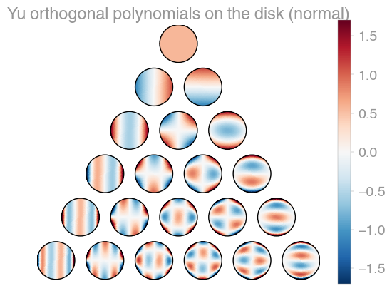
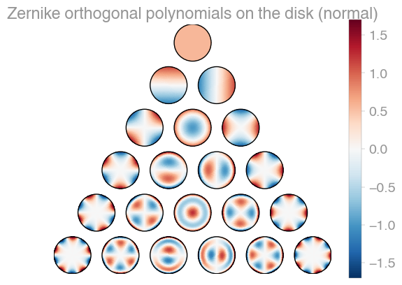
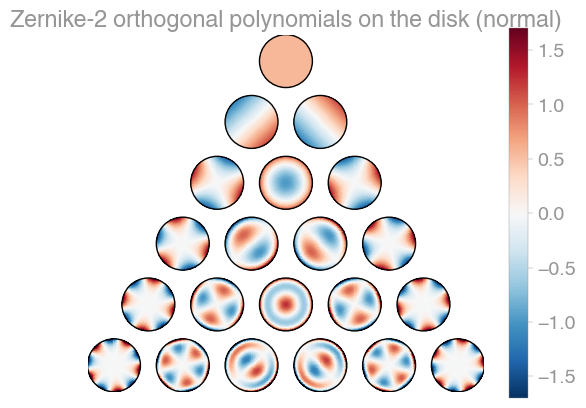
| Xu | [Zernike](https://en.wikipedia.org/wiki/Zernike_polynomials) | Zernike 2 |
orthopy contains several families of orthogonal polynomials on the unit disk: After
[Xu](https://arxiv.org/abs/1701.02709),
[Zernike](https://en.wikipedia.org/wiki/Zernike_polynomials), and a simplified version
of Zernike polynomials.
```python
import orthopy
x = [0.1, -0.3]
evaluator = orthopy.s2.xu.Eval(x, "normal")
# evaluator = orthopy.s2.zernike.Eval(x, "normal")
# evaluator = orthopy.s2.zernike2.Eval(x, "normal")
```
### Sphere (_U3_)
|
| :------------------------------------------------------------------------------------------------: | :-----------------------------------------------------------------------------------------------------: | :------------------------------------------------------------------------------------------------------: |
| Xu | [Zernike](https://en.wikipedia.org/wiki/Zernike_polynomials) | Zernike 2 |
orthopy contains several families of orthogonal polynomials on the unit disk: After
[Xu](https://arxiv.org/abs/1701.02709),
[Zernike](https://en.wikipedia.org/wiki/Zernike_polynomials), and a simplified version
of Zernike polynomials.
```python
import orthopy
x = [0.1, -0.3]
evaluator = orthopy.s2.xu.Eval(x, "normal")
# evaluator = orthopy.s2.zernike.Eval(x, "normal")
# evaluator = orthopy.s2.zernike2.Eval(x, "normal")
```
### Sphere (_U3_)
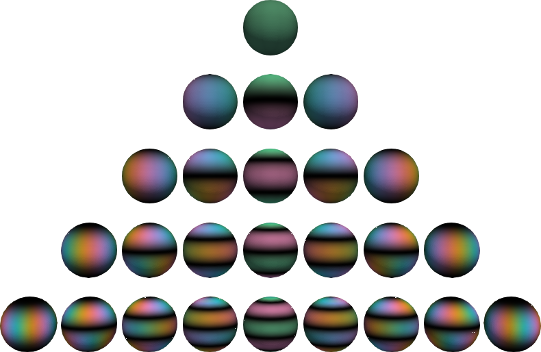 Complex-valued _spherical harmonics,_ (black=zero, green=real positive,
pink=real negative, blue=imaginary positive, yellow=imaginary negative). The
functions in the middle are real-valued. The complex angle takes _n_ turns on
the nth level.
```python
evaluator = orthopy.u3.EvalCartesian(
x,
scaling="quantum mechanic" # or "acoustic", "geodetic", "schmidt"
)
evaluator = orthopy.u3.EvalSpherical(
theta_phi, # polar, azimuthal angles
scaling="quantum mechanic" # or "acoustic", "geodetic", "schmidt"
)
```
### _n_-Cube (_Cn_)
|
Complex-valued _spherical harmonics,_ (black=zero, green=real positive,
pink=real negative, blue=imaginary positive, yellow=imaginary negative). The
functions in the middle are real-valued. The complex angle takes _n_ turns on
the nth level.
```python
evaluator = orthopy.u3.EvalCartesian(
x,
scaling="quantum mechanic" # or "acoustic", "geodetic", "schmidt"
)
evaluator = orthopy.u3.EvalSpherical(
theta_phi, # polar, azimuthal angles
scaling="quantum mechanic" # or "acoustic", "geodetic", "schmidt"
)
```
### _n_-Cube (_Cn_)
|  |
|  |
|  |
| :---------------------------------------------------------------------------------------: | :---------------------------------------------------------------------------------------: | :---------------------------------------------------------------------------------------: |
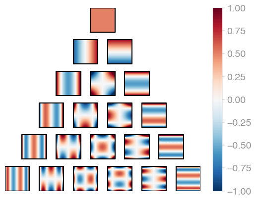
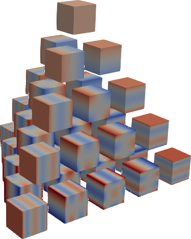
| C1 (Legendre) | C2 | C3 |
Jacobi product polynomials.
All polynomials are normalized on the n-dimensional cube. The dimensionality is
determined by `X.shape[0]`.
```python
evaluator = orthopy.cn.Eval(X, alpha=0, beta=0)
values, degrees = next(evaluator)
```
### nD space with weight function exp(-r2) (_Enr2_)
| |
|
| :---------------------------------------------------------------------------------------: | :---------------------------------------------------------------------------------------: | :---------------------------------------------------------------------------------------: |
| C1 (Legendre) | C2 | C3 |
Jacobi product polynomials.
All polynomials are normalized on the n-dimensional cube. The dimensionality is
determined by `X.shape[0]`.
```python
evaluator = orthopy.cn.Eval(X, alpha=0, beta=0)
values, degrees = next(evaluator)
```
### nD space with weight function exp(-r2) (_Enr2_)
| |  |
|  |
| :-----------------------------------------------------------------------------------------: | :-----------------------------------------------------------------------------------------: | :-----------------------------------------------------------------------------------------: |
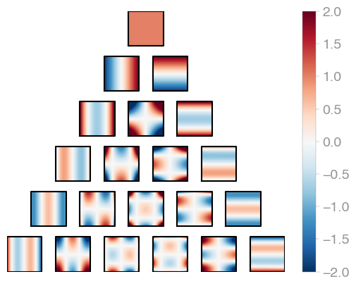
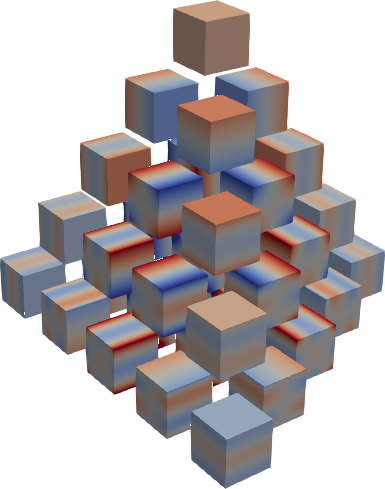
| _E1r2_ | _E2r2_ | _E3r2_ |
Hermite product polynomials.
All polynomials are normalized over the measure. The dimensionality is determined by
`X.shape[0]`.
```python
evaluator = orthopy.enr2.Eval(
x,
standardization="probabilists" # or "physicists"
)
values, degrees = next(evaluator)
```
### Other tools
- Generating recurrence coefficients for 1D domains with
[Stieltjes](https://github.com/nschloe/orthopy/wiki/Generating-1D-recurrence-coefficients-for-a-given-weight#stieltjes),
[Golub-Welsch](https://github.com/nschloe/orthopy/wiki/Generating-1D-recurrence-coefficients-for-a-given-weight#golub-welsch),
[Chebyshev](https://github.com/nschloe/orthopy/wiki/Generating-1D-recurrence-coefficients-for-a-given-weight#chebyshev), and
[modified
Chebyshev](https://github.com/nschloe/orthopy/wiki/Generating-1D-recurrence-coefficients-for-a-given-weight#modified-chebyshev).
- The the sanity of recurrence coefficients with test 3 from [Gautschi's article](https://doi.org/10.1007/BF02218441):
computing the weighted sum of orthogonal polynomials:
```python
orthopy.tools.gautschi_test_3(moments, alpha, beta)
```
- [Clenshaw algorithm](https://en.wikipedia.org/wiki/Clenshaw_algorithm) for
computing the weighted sum of orthogonal polynomials:
```python
vals = orthopy.c1.clenshaw(a, alpha, beta, t)
```
### Relevant publications
- [Robert C. Kirby, Singularity-free evaluation of collapsed-coordinate orthogonal polynomials, ACM Transactions on Mathematical Software (TOMS), Volume 37, Issue 1, January 2010](https://doi.org/10.1145/1644001.1644006)
- [Abedallah Rababah, Recurrence Relations for Orthogonal Polynomials on Triangular Domains, MDPI Mathematics 2016, 4(2)](https://doi.org/10.3390/math4020025)
- [Yuan Xu, Orthogonal polynomials of several variables, arxiv.org, January 2017](https://arxiv.org/abs/1701.02709)
|
| :-----------------------------------------------------------------------------------------: | :-----------------------------------------------------------------------------------------: | :-----------------------------------------------------------------------------------------: |
| _E1r2_ | _E2r2_ | _E3r2_ |
Hermite product polynomials.
All polynomials are normalized over the measure. The dimensionality is determined by
`X.shape[0]`.
```python
evaluator = orthopy.enr2.Eval(
x,
standardization="probabilists" # or "physicists"
)
values, degrees = next(evaluator)
```
### Other tools
- Generating recurrence coefficients for 1D domains with
[Stieltjes](https://github.com/nschloe/orthopy/wiki/Generating-1D-recurrence-coefficients-for-a-given-weight#stieltjes),
[Golub-Welsch](https://github.com/nschloe/orthopy/wiki/Generating-1D-recurrence-coefficients-for-a-given-weight#golub-welsch),
[Chebyshev](https://github.com/nschloe/orthopy/wiki/Generating-1D-recurrence-coefficients-for-a-given-weight#chebyshev), and
[modified
Chebyshev](https://github.com/nschloe/orthopy/wiki/Generating-1D-recurrence-coefficients-for-a-given-weight#modified-chebyshev).
- The the sanity of recurrence coefficients with test 3 from [Gautschi's article](https://doi.org/10.1007/BF02218441):
computing the weighted sum of orthogonal polynomials:
```python
orthopy.tools.gautschi_test_3(moments, alpha, beta)
```
- [Clenshaw algorithm](https://en.wikipedia.org/wiki/Clenshaw_algorithm) for
computing the weighted sum of orthogonal polynomials:
```python
vals = orthopy.c1.clenshaw(a, alpha, beta, t)
```
### Relevant publications
- [Robert C. Kirby, Singularity-free evaluation of collapsed-coordinate orthogonal polynomials, ACM Transactions on Mathematical Software (TOMS), Volume 37, Issue 1, January 2010](https://doi.org/10.1145/1644001.1644006)
- [Abedallah Rababah, Recurrence Relations for Orthogonal Polynomials on Triangular Domains, MDPI Mathematics 2016, 4(2)](https://doi.org/10.3390/math4020025)
- [Yuan Xu, Orthogonal polynomials of several variables, arxiv.org, January 2017](https://arxiv.org/abs/1701.02709)