{
"cells": [
{
"cell_type": "markdown",
"metadata": {},
"source": [
"# EM Notebooks\n",
"\n",
" \n",
"\n",
"A collection of notebooks that use the electromagnetics (EM) module of [SimPEG](http://simpeg.xyz). Many of these notebooks reproduce examples from [EM GeoSci](http://em.geosci.xyz), an open source “textbook” on applied electromagnetics.\n",
"\n",
"\n",
"If you build upon these notebooks in your work, please cite:\n",
"\n",
"- [(Cockett et al., 2015)](http://www.sciencedirect.com/science/article/pii/S009830041530056X): *SimPEG: An open source framework for simulation and gradient based parameter estimation in geophysical applications*\n",
"- [(Heagy et al., 2016)](https://arxiv.org/abs/1610.00804): *A framework for simulation and inversion in electromagnetics*\n",
"\n",
"If you have feedback, we would like to hear from you! \n",
"- Contact us\n",
"- Report issues\n",
"- Join the development\n"
]
},
{
"cell_type": "markdown",
"metadata": {},
"source": [
"**[EM Fundamentals](#EM-Fundamentals) | [Inverting Field Data](Inverting-Field-Data) | [MT Tutorial](#MT-Tutorial) | [Additional Notebooks](#Additional-Notebooks)**\n",
"\n",
"## Contents\n",
"\n",
"### EM Fundamentals\n",
"\n",
"These notebooks walk through using SimPEG for conducting a TDEM and FDEM soundings over a sphere. They use the cylindrically symmetric mesh for the forward modelling\n",
"- [TDEM_vmd_sounding_over_sphere.ipynb](notebooks/TDEM_vmd_sounding_over_sphere.ipynb)\n",
"- [FDEM_vmd_sounding_over_sphere.ipynb](notebooks/FDEM_vmd_sounding_over_sphere.ipynb)\n",
"\n",
"\n",
"### Inverting Field Data\n",
"\n",
"These notebooks walk through inverting a single sounding of airborne EM data collected in Australia. \n",
"- [TDEM_inversion_bookpurnong](notebooks/TDEM_inversion_bookpurnong.ipynb)\n",
"- [FDEM_inversion_bookpurnong](notebooks/FDEM_inversion_bookpurnong.ipynb)\n",
"\n",
"### MT Tutorial\n",
"\n",
"These notebooks were originall published in [The Leading Edge](https://doi.org/10.1190/tle36080696.1)\n",
"\n",
" Seogi Kang , Lindsey J. Heagy , Rowan Cockett , and Douglas W. Oldenburg (2017). ”Exploring nonlinear inversions: A 1D magnetotelluric example.” The Leading Edge, 36(8), 696–699.\n",
"\n",
"\n",
"There are 5 notebooks in this tutorial - we wrote them starting from discretizing the governing equations for the Magnetotelluric Problem, running a forward simulation and exploring an example of non-uniqueness, and performing the inversion. Although this is a natural order in terms of building the pieces, you do not need to work through them in order, each notebook is self-contained and has links to others where appropriate. \n",
"\n",
"- [1_MT1D_NumericalSetup](notebooks/MT_tutorial_1_MT1D_NumericalSetup.ipynb): discretize and solve the 1D MT equations \n",
"- [2_MT1D_ForwardModellingAndNonuniqueness](notebooks/MT_tutorial_2_MT1D_ForwardModellingAndNonuniqueness.ipynb): run the forward simulation and explore an example of non-uniqueness\n",
"- [3_MT1D_5layer_inversion](notebooks/MT_tutorial_3_MT1D_5layer_inversion.ipynb): run inversions for a 5 layer model and explore the impacts of choosing a trade-off parameter $\\beta$, and changing the regularization parameters smoothness and smallness ($\\alpha_s$ and $\\alpha_z$). \n",
"\n",
"There are also 2 \"appendix\" notebooks\n",
"- [Appendix_A_MT1D_Sensitivity](notebooks/MT_tutorial_Appendix_A_MT1D_Sensitivity.ipynb): derive and test the sensitivity \n",
"- [Appendix_B_MT1D_tests](notebooks/MT_tutorial_Appendix_B_MT1D_tests.ipynb): demonstrates how we test the code\n",
"\n",
"\n",
"### Additional Notebooks\n",
"- [DC_Mise-a-la-masse.ipynb](notebooks/DC_Mise-a-la-masse.ipynb)\n",
"- [DC_inversion_2D_example.ipynb](notebooks/DC_inversion_2D_example.ipynb)\n",
"- [FDEM_target_in_solenoid.ipynb](notebooks/FDEM_target_in_solenoid.ipynb)\n",
"- [TDEM_1D_inversion.ipynb](notebooks/TDEM_1D_inversion.ipynb)"
]
},
{
"cell_type": "markdown",
"metadata": {},
"source": [
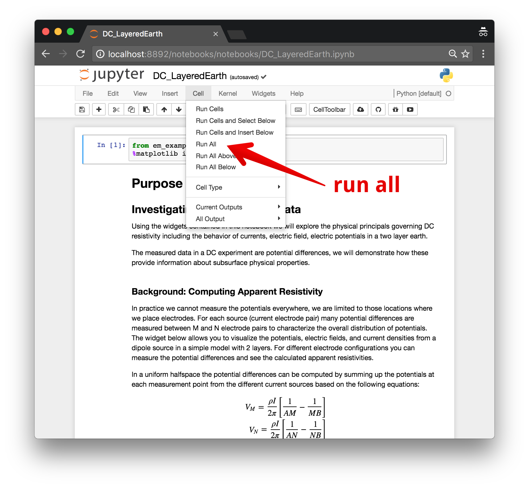
"## Running the notebook\n",
"\n",
"From the menu, select `cell`, `run all`, or run each individual cell using `shift + enter`\n",
"\n",
"\n",
"\n",
"If you want to start with a clean slate, restart the Kernel either by going to the top, clicking on Kernel: Restart, or by \"esc + 00\" (if you do this, you will need to re-run the following block of code before running any other cells in the notebook) \n",
"\n",
"For more information on running Jupyter notebooks, see the [Jupyter Documentation](https://jupyter.readthedocs.io/en/latest/)"
]
},
{
"cell_type": "code",
"execution_count": null,
"metadata": {},
"outputs": [],
"source": []
}
],
"metadata": {
"anaconda-cloud": {},
"kernelspec": {
"display_name": "Python 3",
"language": "python",
"name": "python3"
},
"language_info": {
"codemirror_mode": {
"name": "ipython",
"version": 3
},
"file_extension": ".py",
"mimetype": "text/x-python",
"name": "python",
"nbconvert_exporter": "python",
"pygments_lexer": "ipython3",
"version": "3.6.6"
}
},
"nbformat": 4,
"nbformat_minor": 1
}
\n",
"\n",
"A collection of notebooks that use the electromagnetics (EM) module of [SimPEG](http://simpeg.xyz). Many of these notebooks reproduce examples from [EM GeoSci](http://em.geosci.xyz), an open source “textbook” on applied electromagnetics.\n",
"\n",
"\n",
"If you build upon these notebooks in your work, please cite:\n",
"\n",
"- [(Cockett et al., 2015)](http://www.sciencedirect.com/science/article/pii/S009830041530056X): *SimPEG: An open source framework for simulation and gradient based parameter estimation in geophysical applications*\n",
"- [(Heagy et al., 2016)](https://arxiv.org/abs/1610.00804): *A framework for simulation and inversion in electromagnetics*\n",
"\n",
"If you have feedback, we would like to hear from you! \n",
"- Contact us\n",
"- Report issues\n",
"- Join the development\n"
]
},
{
"cell_type": "markdown",
"metadata": {},
"source": [
"**[EM Fundamentals](#EM-Fundamentals) | [Inverting Field Data](Inverting-Field-Data) | [MT Tutorial](#MT-Tutorial) | [Additional Notebooks](#Additional-Notebooks)**\n",
"\n",
"## Contents\n",
"\n",
"### EM Fundamentals\n",
"\n",
"These notebooks walk through using SimPEG for conducting a TDEM and FDEM soundings over a sphere. They use the cylindrically symmetric mesh for the forward modelling\n",
"- [TDEM_vmd_sounding_over_sphere.ipynb](notebooks/TDEM_vmd_sounding_over_sphere.ipynb)\n",
"- [FDEM_vmd_sounding_over_sphere.ipynb](notebooks/FDEM_vmd_sounding_over_sphere.ipynb)\n",
"\n",
"\n",
"### Inverting Field Data\n",
"\n",
"These notebooks walk through inverting a single sounding of airborne EM data collected in Australia. \n",
"- [TDEM_inversion_bookpurnong](notebooks/TDEM_inversion_bookpurnong.ipynb)\n",
"- [FDEM_inversion_bookpurnong](notebooks/FDEM_inversion_bookpurnong.ipynb)\n",
"\n",
"### MT Tutorial\n",
"\n",
"These notebooks were originall published in [The Leading Edge](https://doi.org/10.1190/tle36080696.1)\n",
"\n",
" Seogi Kang , Lindsey J. Heagy , Rowan Cockett , and Douglas W. Oldenburg (2017). ”Exploring nonlinear inversions: A 1D magnetotelluric example.” The Leading Edge, 36(8), 696–699.\n",
"\n",
"\n",
"There are 5 notebooks in this tutorial - we wrote them starting from discretizing the governing equations for the Magnetotelluric Problem, running a forward simulation and exploring an example of non-uniqueness, and performing the inversion. Although this is a natural order in terms of building the pieces, you do not need to work through them in order, each notebook is self-contained and has links to others where appropriate. \n",
"\n",
"- [1_MT1D_NumericalSetup](notebooks/MT_tutorial_1_MT1D_NumericalSetup.ipynb): discretize and solve the 1D MT equations \n",
"- [2_MT1D_ForwardModellingAndNonuniqueness](notebooks/MT_tutorial_2_MT1D_ForwardModellingAndNonuniqueness.ipynb): run the forward simulation and explore an example of non-uniqueness\n",
"- [3_MT1D_5layer_inversion](notebooks/MT_tutorial_3_MT1D_5layer_inversion.ipynb): run inversions for a 5 layer model and explore the impacts of choosing a trade-off parameter $\\beta$, and changing the regularization parameters smoothness and smallness ($\\alpha_s$ and $\\alpha_z$). \n",
"\n",
"There are also 2 \"appendix\" notebooks\n",
"- [Appendix_A_MT1D_Sensitivity](notebooks/MT_tutorial_Appendix_A_MT1D_Sensitivity.ipynb): derive and test the sensitivity \n",
"- [Appendix_B_MT1D_tests](notebooks/MT_tutorial_Appendix_B_MT1D_tests.ipynb): demonstrates how we test the code\n",
"\n",
"\n",
"### Additional Notebooks\n",
"- [DC_Mise-a-la-masse.ipynb](notebooks/DC_Mise-a-la-masse.ipynb)\n",
"- [DC_inversion_2D_example.ipynb](notebooks/DC_inversion_2D_example.ipynb)\n",
"- [FDEM_target_in_solenoid.ipynb](notebooks/FDEM_target_in_solenoid.ipynb)\n",
"- [TDEM_1D_inversion.ipynb](notebooks/TDEM_1D_inversion.ipynb)"
]
},
{
"cell_type": "markdown",
"metadata": {},
"source": [
"## Running the notebook\n",
"\n",
"From the menu, select `cell`, `run all`, or run each individual cell using `shift + enter`\n",
"\n",
"\n",
"\n",
"If you want to start with a clean slate, restart the Kernel either by going to the top, clicking on Kernel: Restart, or by \"esc + 00\" (if you do this, you will need to re-run the following block of code before running any other cells in the notebook) \n",
"\n",
"For more information on running Jupyter notebooks, see the [Jupyter Documentation](https://jupyter.readthedocs.io/en/latest/)"
]
},
{
"cell_type": "code",
"execution_count": null,
"metadata": {},
"outputs": [],
"source": []
}
],
"metadata": {
"anaconda-cloud": {},
"kernelspec": {
"display_name": "Python 3",
"language": "python",
"name": "python3"
},
"language_info": {
"codemirror_mode": {
"name": "ipython",
"version": 3
},
"file_extension": ".py",
"mimetype": "text/x-python",
"name": "python",
"nbconvert_exporter": "python",
"pygments_lexer": "ipython3",
"version": "3.6.6"
}
},
"nbformat": 4,
"nbformat_minor": 1
}