{
"cells": [
{
"cell_type": "markdown",
"metadata": {},
"source": [
"# A simple economic model with an analytical solution\n",
"\n",
"In this notebook, we use `TensorFlow 1.13.1` to showcase the general workflow of setting up and solving dynamic general equilibrium models with _deep equilibrium nets_. Use `pip install tensorflow==1.13.1` to install the correct version.\n",
"\n",
"The notebook accompanies the working paper by [Azinovic, Gaegauf, & Scheidegger (2021)](https://papers.ssrn.com/sol3/papers.cfm?abstract_id=3393482) and corresponds to the model solved in appendix H with a slighly different model calibration.\n",
"\n",
"Note that this is a minimal working example for illustration purposes only. A more extensive implementation will be published on Github. \n",
"\n",
"The economic model we are solving in this example is one for which we know an exact solution. We chose to solve a model from [Krueger and Kubler (2004)](https://www.sciencedirect.com/science/article/pii/S0165188903001118), which is based on [Huffman (1987)](https://www.journals.uchicago.edu/doi/10.1086/261445), because, in addition to being analytically solvable, it is closely related to the models solved in the paper. Therefore, the approach presented in this notebook translates directly to the models in working paper.\n",
"\n",
"## The model \n",
"\n",
"We outline the model briefly. \n",
"\n",
"### tldr\n",
"The model has $A$ agents that only work in the first period of their lives. They optimize lifetime log utility by saving in risky capital. Agents consume everything in the last period. There is a representative firm that produces with labor and capital and is affected by TFP and depreciation shocks. The firm pays market prices for labor and capital.\n",
"\n",
"***\n",
"\n",
"### Households\n",
"Agents live for $A$ (here we consider $A = 6$) periods and have log utility. Agents only work in the first period of their life: $l^h_t=1$ for $h=0$ and $l^h_t=0$ otherwise. Therefore, the aggregate labor supply is constant and equal to one: $L_t=1$. Agents receive a competitive wage and can save in risky capital. Households cannot die with debt. Otherwise, there are no constraints or adjustment costs.\n",
"The household's problem is\n",
"\n",
"$$ \\max_{\\{c_{t+i}^{i}, a_{t+i}^{i}\\}_{i=0}^{A-1}}\\mathbb{E}_{t}{\\sum_{i=0}^{A-1}\\log(c_{t+i}^{i})} $$\n",
"subject to:\n",
"$$c_{t}^{h} + a_t^{h} = r_t k_t^h + w_t l^h_t$$\n",
"$$k^{h+1}_{t+1} = a_t^h $$\n",
"$$a^{A-1}_t \\geq 0$$\n",
"\n",
"where $c_t^h$ denotes the consumption of age-group $h$ at time $t$, $a^h_t$ denotes the saving, $k_t^h$ denotes the available capital in the beginning of the period, $r_t$ denotes the price of capital, $l_t^h$ denotes the exogenously supplied labor endowment, and $w_t$ denotes the wage.\n",
"\n",
"### Firms\n",
"\n",
"There is a single representative firm with Cobb-Douglas production function.\n",
"The production function is given by\n",
"$$f(K_t,L_t,z_t) = \\eta_t K^{\\alpha}_t L^{1-\\alpha}_t + K_t(1-\\delta_t),$$\n",
"where $K_t$ denotes aggregate capital, where\n",
"$$K_t = \\sum_{h=0}^{A-1} k^h_t,$$\n",
"$L_t$ denotes the aggregate labor supply, where\n",
"$$L_t = \\sum_{h=0}^{A-1} l^h_t,$$\n",
"$\\alpha$ denotes the capital share in production, $\\eta_t$ denotes the stochastic TFP, and $\\delta_t$ denotes the stochastic depreciation. The firm's optimization problem implies that the return on capital and the wage are given by\n",
"$$r_t = \\alpha \\eta_t K_t^{\\alpha - 1} L_t^{1 - \\alpha} + (1 - \\delta_t),$$\n",
"$$w_t = (1 - \\alpha) \\eta_t K_t^{\\alpha} L_t^{-\\alpha}.$$\n",
"\n",
"## Equilibrium\n",
"\n",
"A competitive equilibrium, given initial conditions $z_0, \\{ k_0^s \\}_{s=0}^{A-1}$, is a collection of choices for households $ \\{ (c_t^s, a_t^s)_{s = 0}^{A-1} \\}_{t=0}^\\infty$ and for the representative firm $(K_t, L_t)_{t=0}^\\infty$ as well as prices $(r_t, w_t)_{t=0}^\\infty$, such that\n",
"\n",
"1. given prices, households optimize,\n",
"2. given prices, the firm maximizes profits,\n",
"3. markets clear.\n",
"\n",
"\n",
"## Table of contents\n",
"\n",
"0. [Set up workspace](#workspace)\n",
"1. [Model calibration](#modelcal)\n",
"2. [_Deep equilibrium net_ hyper-parameters](#deqnparam)\n",
" 1. [Neural network](#nn)\n",
"3. [Economic model](#econmodel)\n",
" 1. [Current period (t)](#currentperiod)\n",
" 2. [Next period (t+1)](#nextperiod)\n",
" 3. [Cost/Euler function](#cost)\n",
"4. [Training](#training)"
]
},
{
"cell_type": "markdown",
"metadata": {},
"source": [
"## 0. Set up workspace \n",
"\n",
"First, we need to set up the workspace. All of the packages are standard python packages. This version of the _deep equilibrium net_ notebook will be computed with `TensorFlow 1.13.1`. Make sure you are working in an environment with TF1 installed. Use `pip install tensorflow==1.13.1` to install the correct version.\n",
"\n",
"The only special module is `utils` from which we import a mini-batch function `random_mini_batches` and a function that initializes the neural network weights `initialize_nn_weight`.\n",
"\n",
"### Saving and continuing training\n",
"\n",
"You can save and resume training by saving and loading the tensorflow session and data starting point.\n",
"* The saved session stores the neural network weights and the optimizer's state. If you have saved a session that you would like to reload, set `sess_path` to the session checkpoint path. For example, to load the 100th episode's session set `sess_path = './output/sess_100.ckpt'`. Otherwise, set `sess_path` to `None` to train from scratch. Currently, this script saves the session at the end of each [episode](#deqnparam).\n",
"* The saved data starting point stores the an exogeneous shock and a capital distribution, which can be used to simulate states into the future from. If you have saved a starting point that you would like to reload, set `data_path` to the numpy data path. For example, to load the 100th episode's starting point set `data_path = './output/data_100.npy'`. Otherwise, set `data_path` to `None` to train from scratch."
]
},
{
"cell_type": "code",
"execution_count": 5,
"metadata": {
"scrolled": true
},
"outputs": [
{
"name": "stdout",
"output_type": "stream",
"text": [
"tf version: 1.13.1\n"
]
}
],
"source": [
"%matplotlib notebook\n",
"\n",
"# Import modules\n",
"import os\n",
"import re\n",
"from datetime import datetime\n",
"\n",
"import tensorflow as tf\n",
"import numpy as np\n",
"from utils import initialize_nn_weight, random_mini_batches\n",
"\n",
"import matplotlib.pyplot as plt\n",
"plt.rcParams.update({'font.size': 12})\n",
"plt.rc('xtick', labelsize='small')\n",
"plt.rc('ytick', labelsize='small')\n",
"std_figsize = (4, 4)\n",
"\n",
"# Make sure that we are working with tensorflow 1\n",
"print('tf version:', tf.__version__)\n",
"assert tf.__version__[0] == '1'\n",
"\n",
"# Set the seed for replicable results\n",
"seed = 0\n",
"np.random.seed(seed)\n",
"tf.set_random_seed(seed)\n",
"\n",
"# Helper variables\n",
"eps = 0.00001 # Small epsilon value\n",
"\n",
"# Make output directory to save network weights and starting point\n",
"if not os.path.exists('./output'):\n",
" os.mkdir('./output')\n",
"\n",
"# Path to saved tensorflow session\n",
"sess_path = None\n",
"# Path to saved data starting point\n",
"data_path = None"
]
},
{
"cell_type": "markdown",
"metadata": {},
"source": [
"## 1. Model calibration \n",
"\n",
"### tldr\n",
"\n",
"We solve a model with 6 agents. There are 4 exogenous shock which are the product of 2 depreciation ($\\delta \\in \\{0.5, 0.9\\}$) and 2 TFP shocks ($\\eta \\in \\{0.95, 1.05\\}$). Each shock-state has an equal probably of 0.25 of realizing in the next period. Agents only work in the first period. The economic parameters are calibrated to: $\\alpha = 0.3$, $\\beta=0.7$, and $\\gamma = 1.0$.\n",
"\n",
"***\n",
"\n",
"We solve the model for $A = 6$ agents and base our parameterization on [Krueger and Kubler (2004)](https://www.sciencedirect.com/science/article/pii/S0165188903001118). \n",
"\n",
"### Shocks\n",
"The depreciation $\\delta$ takes one of two values, $\\delta \\in \\{0.5, 0.9\\}$. The TFP $\\eta$ also takes one of two values, $\\eta \\in \\{0.95, 1.05\\}$.\n",
"Both the TFP and depreciation shocks are i.i.d. with a transition matrix:\n",
"\\begin{equation}\n",
"\\Pi^{\\eta} = \\Pi^{\\delta}=\n",
"\\begin{bmatrix}\n",
"0.5 & 0.5 \\\\\n",
"0.5 & 0.5\n",
"\\end{bmatrix}.\n",
"\\end{equation}\n",
"and evolve independently of each other. In total, there are four possible combinations of depreciation shock and TFP shock that are labeled by $z \\in \\mathcal{Z}=\\{1,2,3,4\\}$ and correspond to $\\delta=[0.5, 0.5, 0.9, 0.9]^T$ and $\\eta=[0.95, 1.05, 0.95, 1.05]^T$. The overall transition matrix is given by\n",
"\\begin{equation}\n",
"\\Pi= \\Pi^{\\delta} \\otimes \\Pi^{\\eta} = \\begin{bmatrix}\n",
"0.25 & 0.25 & 0.25 & 0.25 \\\\\n",
"0.25 & 0.25 & 0.25 & 0.25 \\\\\n",
"0.25 & 0.25 & 0.25 & 0.25 \\\\\n",
"0.25 & 0.25 & 0.25 & 0.25\n",
"\\end{bmatrix},\n",
"\\end{equation} where $\\Pi_{i, j}$ denotes the probability of a transition from the exogenous shock $i$ to exogenous shock $j$, where $i,j \\in \\mathcal{Z}$. \n",
"\n",
"### Labor\n",
"Agents in this economy are alive for 6 periods. Agents work in the first period of their lives before retiring for the remaining 4. That is, their labor endowment during their working age is 1 (and 0 otherwise).\n",
"\n",
"### Production and household parameters\n",
"The output elasticity of the Cobb-Douglas production function is $\\alpha = 0.3$, the discount factor of agents' utility is $\\beta=0.7$, and the coeffient of risk aversion (in CRRA utility) is $\\gamma = 1.0$.\n"
]
},
{
"cell_type": "code",
"execution_count": 8,
"metadata": {},
"outputs": [],
"source": [
"# Number of agents and exogenous shocks\n",
"num_agents = A = 6\n",
"num_exogenous_shocks = 4\n",
"\n",
"# Exogenous shock values\n",
"delta = tf.constant([[0.5], [0.5], [0.9], [0.9]], dtype=tf.float32) # Capital depreciation (dependent on shock)\n",
"eta = tf.constant([[0.95], [1.05], [0.95], [1.05]], dtype=tf.float32) # TFP shock (dependent on shock)\n",
"\n",
"# Transition matrix\n",
"# In this example we hardcoded the transition matrix. Changes cannot be made without also changing\n",
"# the corresponding code below.\n",
"p_transition = 0.25 # All transition probabilities are 0.25\n",
"pi_np = p_transition * np.ones((4, 4)) # Transition probabilities\n",
"pi = tf.constant(pi_np, dtype=tf.float32) # Transition probabilities\n",
"\n",
"# Labor endowment\n",
"labor_endow_np = np.zeros((1, A))\n",
"labor_endow_np[:, 0] = 1.0 # Agents only work in their first period\n",
"labor_endow = tf.constant(labor_endow_np, dtype=tf.float32)\n",
"\n",
"# Production and household parameters\n",
"alpha = tf.constant(0.3) # Capital share in production\n",
"beta_np = 0.7\n",
"beta = tf.constant(beta_np, dtype=tf.float32) # Discount factor (patience)\n",
"gamma = tf.constant(1.0, dtype=tf.float32) # CRRA coefficient"
]
},
{
"cell_type": "markdown",
"metadata": {},
"source": [
"## 2. _Deep equilibrium net_ hyper-parameters \n",
"\n",
"Here, we will briefly outline the _deep equilibrium net_ architecture and choice of hyper-parameters. By hyper-parameters, we refer too all of the parameters that can be chosen freely by the modeller. This is in contrast to \"parameters\", which refers to the neural network weights that are learned during training.\n",
"We found it helpful to augment the state we pass to the neural network with redundant information, such as aggregate variables and the distribution of financial wealth.\n",
"In this notebook, we do the same.\n",
"\n",
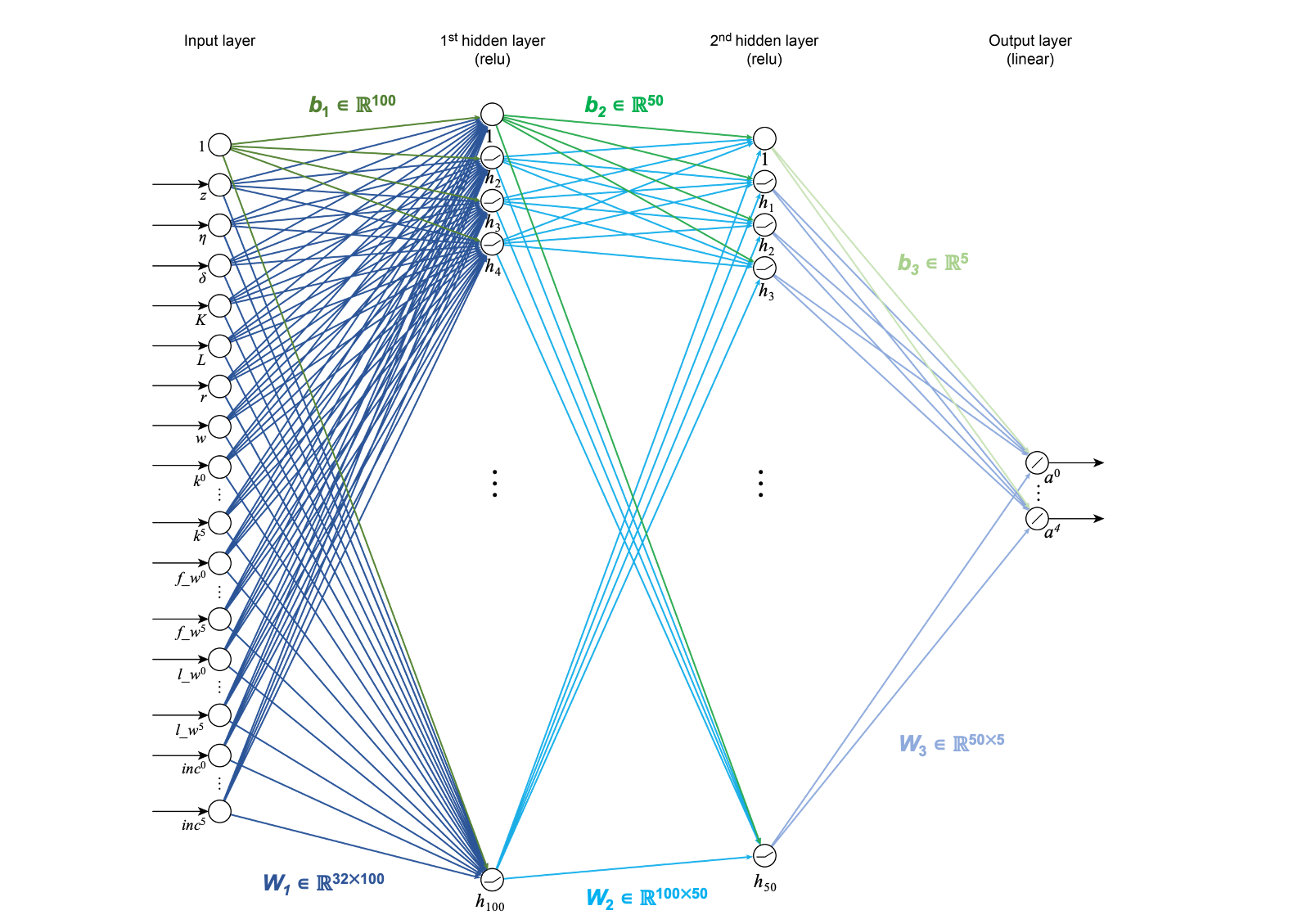
" * Neural network architecture (see NN diagram below):\n",
" * The neural network takes an extended state that is 32-dimensional:\n",
" * Natural state:\n",
" * 1 dimension for the shock index,\n",
" * 6 dimensions for the distribution of capital across age groups\n",
" * Redundant extension:\n",
" * 1 dimension for the current TFP,\n",
" * 1 dimension for the current depreciation,\n",
" * 1 dimension for aggregate capital,\n",
" * 1 dimension for aggregate labor supply, \n",
" * 1 dimension for the return on capital,\n",
" * 1 dimension for the wage,\n",
" * 1 dimension for the aggregate production,\n",
" * 6 dimensions for the distribution of financial wealth,\n",
" * 6 dimensions for the distribution of labor income, \n",
" * 6 dimensions for the distribution of total income.\n",
" * The first and second hidden layers have 100 and 50 nodes, respectively.\n",
" * The output layer is 5-dimensional.\n",
" * Training hyper-parameters:\n",
" * We simulate 5'000 episodes.*\n",
" * Per episode, we compute 20 epochs.\n",
" * We use a minibatch size of 512.\n",
" * Each episode is 10'240 periods long.\n",
" * The learning rate is set to 0.00001.\n",
"\n",
"\\* In the _deep equilibrium net_ framework we iterate between a simulation and training phase (see [training](#training)). We first simulate a training dataset based on the current state of the neural network. That is, we simulate a random sequence of exogenous shocks for which we compute the capital holdings of the agents. We call the set of simulated periods an _episode_. 5'000 episodes means that we re-simulate the training data 5'000 times.\n",
"\n",
"Note that this calibration is not optimal for the economic model being solved. This script is intended to provide a simple introduction to _deep equilibrium nets_ and not an indepth discussion on optimizing the performance.\n",
"\n",
" "
]
},
{
"cell_type": "code",
"execution_count": 9,
"metadata": {},
"outputs": [],
"source": [
"num_episodes = 5000 \n",
"len_episodes = 10240\n",
"epochs_per_episode = 20\n",
"minibatch_size = 512\n",
"num_minibatches = int(len_episodes / minibatch_size)\n",
"lr = 0.00001\n",
"\n",
"# Neural network architecture parameters\n",
"num_input_nodes = 8 + 4 * A # Dimension of extended state space (8 aggregate quantities and 4 distributions)\n",
"num_hidden_nodes = [100, 50] # Dimension of hidden layers\n",
"num_output_nodes = (A - 1) # Output dimension (capital holding for each agent. Agent 1 is born without capital (k^1=0))"
]
},
{
"cell_type": "markdown",
"metadata": {},
"source": [
"### 2.A. Neural network \n",
"\n",
"Since we are using a neural network with 2 hidden layers, the network maps:\n",
"$$X \\rightarrow \\mathcal{N}(X) = \\sigma(\\sigma(XW_1 + b_1)W_2 + b_2)W_3 + b_3$$\n",
"where $\\sigma$ is the rectified linear unit (ReLU) activation function and the output layer is activated with the linear function (which is the identity function and hence omitted from the equation). Therefore, we need 3 weight matrices $\\{W_1, W_2, W_3\\}$ and 3 bias vectors $\\{b_1, b_2, b_3\\}$ (compare with the neural network diagram above). In total, we train 5'954 parameters:\n",
"\n",
"| $W_1$ | $32 \\times 100$ | $= 3200$ |\n",
"| --- | --- | --- |\n",
"| $W_2$ | $100 \\times 50$ | $= 5000$ |\n",
"| $W_3$ | $50 \\times 5$ | $= 250$ |\n",
"| $b_1 + b_2 + b_3$ | $100 + 50 + 5$ | $= 155$|\n",
"\n",
"\n",
"We initialize the neural network parameters with the `initialize_nn_weight` helper function from `utils`.\n",
"\n",
"Then, we compute the neural network prediction using the parameters in `nn_predict`. "
]
},
{
"cell_type": "code",
"execution_count": 14,
"metadata": {},
"outputs": [],
"source": [
"# We create a placeholder for X, the input data for the neural network, which corresponds\n",
"# to the state.\n",
"X = tf.placeholder(tf.float32, shape=(None, num_input_nodes))\n",
"# Get number samples\n",
"m = tf.shape(X)[0]\n",
"\n",
"# We create all of the neural network weights and biases. The weights are matrices that\n",
"# connect the layers of the neural network. For example, W1 connects the input layer to\n",
"# the first hidden layer\n",
"W1 = initialize_nn_weight([num_input_nodes, num_hidden_nodes[0]])\n",
"W2 = initialize_nn_weight([num_hidden_nodes[0], num_hidden_nodes[1]])\n",
"W3 = initialize_nn_weight([num_hidden_nodes[1], num_output_nodes])\n",
"\n",
"# The biases are extra (shift) terms that are added to each node in the neural network.\n",
"b1 = initialize_nn_weight([num_hidden_nodes[0]])\n",
"b2 = initialize_nn_weight([num_hidden_nodes[1]])\n",
"b3 = initialize_nn_weight([num_output_nodes])\n",
"\n",
"# Then, we create a function, to which we pass X, that generates a prediction based on\n",
"# the current neural network weights. Note that the hidden layers are ReLU activated.\n",
"# The output layer is not activated (i.e., it is activated with the linear function).\n",
"def nn_predict(X):\n",
" hidden_layer1 = tf.nn.relu(tf.add(tf.matmul(X, W1), b1))\n",
" hidden_layer2 = tf.nn.relu(tf.add(tf.matmul(hidden_layer1, W2), b2))\n",
" output_layer = tf.add(tf.matmul(hidden_layer2, W3), b3)\n",
" return output_layer\n"
]
},
{
"cell_type": "markdown",
"metadata": {},
"source": [
"## 3. Economic model \n",
"\n",
"In this section, we implement the economics outlined in [the model](#model).\n",
"\n",
"Each period, based on the current distribution of capital and the exogenous state, agents decide whether and how much to save in risky capital and to consume. Their savings together with the labor supplied implies the rest of the economic state (e.g., capital return, wages, incomes, ...). We use the neural network to generate the savings based on the agents' capital holdings at the beginning of the period. The remaining economic state is computed using the equations outlined [above](#model). The economic mechanisms are encoded in helper functions. We create one for the `firm`, the `shocks`, and `wealth` (see cell below).\n",
"\n",
"Then, in the face of future uncertainty, the agents again decide whether and how much to save in risky capital for the next period. We use the neural network to generate new savings for each of the future states (one for each shock). The input state for these network predictions is the next period's capital holding which are current periods savings.\n",
"\n",
"First, we define the helper functions for the `firm`, the `shocks`, and `wealth`.\n"
]
},
{
"cell_type": "code",
"execution_count": 5,
"metadata": {},
"outputs": [],
"source": [
"def firm(K, eta, alpha, delta):\n",
" \"\"\"Calculate return, wage and aggregate production.\n",
" \n",
" r = eta * K^(alpha-1) * L^(1-alpha) + (1-delta)\n",
" w = eta * K^(alpha) * L^(-alpha)\n",
" Y = eta * K^(alpha) * L^(1-alpha) + (1-delta) * K \n",
"\n",
" Args:\n",
" K: aggregate capital,\n",
" eta: TFP value,\n",
" alpha: output elasticity,\n",
" delta: depreciation value.\n",
"\n",
" Returns:\n",
" return: return (marginal product of capital), \n",
" wage: wage (marginal product of labor).\n",
" Y: aggregate production.\n",
" \"\"\"\n",
" L = tf.ones_like(K)\n",
"\n",
" r = alpha * eta * K**(alpha - 1) * L**(1 - alpha) + (1 - delta)\n",
" w = (1 - alpha) * eta * K**alpha * L**(-alpha)\n",
" Y = eta * K**alpha * L**(1 - alpha) + (1 - delta) * K\n",
"\n",
" return r, w, Y\n",
"\n",
"def shocks(z, eta, delta):\n",
" \"\"\"Calculates tfp and depreciation based on current exogenous shock.\n",
"\n",
" Args:\n",
" z: current exogenous shock (in {1, 2, 3, 4}),\n",
" eta: tensor of TFP values to sample from,\n",
" delta: tensor of depreciation values to sample from.\n",
"\n",
" Returns:\n",
" tfp: TFP value of exogenous shock, \n",
" depreciation: depreciation values of exogenous shock.\n",
" \"\"\"\n",
" tfp = tf.gather(eta, tf.cast(z, tf.int32))\n",
" depreciation = tf.gather(delta, tf.cast(z, tf.int32))\n",
" return tfp, depreciation\n",
" \n",
"def wealth(k, R, l, W):\n",
" \"\"\"Calculates the wealth of the agents.\n",
"\n",
" Args:\n",
" k: capital distribution,\n",
" R: matrix of return,\n",
" l: labor distribution,\n",
" W: matrix of wages.\n",
"\n",
" Returns:\n",
" fin_wealth: financial wealth distribution,\n",
" lab_wealth: labor income distribution,\n",
" tot_income: total income distribution.\n",
" \"\"\"\n",
" fin_wealth = k * R\n",
" lab_wealth = l * W\n",
" tot_income = tf.add(fin_wealth, lab_wealth)\n",
" return fin_wealth, lab_wealth, tot_income\n"
]
},
{
"cell_type": "markdown",
"metadata": {},
"source": [
"### 3.A. Current period (t) \n",
"Using the current state `X` we can calculate the economy. The state is composed of today's shock ($z_t$) and today's capital ($k_t^h$). Note that this constitutes the minimal state. Often, including redundant variables is a simple way to increase the speed of convergence (see the [working paper](https://papers.ssrn.com/sol3/papers.cfm?abstract_id=3393482) for more information on this). However, this notebook attempts to present the most basic example for simplicity.\n",
"\n",
"Using the current state `X`, we predict how much the agents save ($a_t^h$) based on their current capital holdings ($k_t^h$). We do this by passing the state `X` to the neural network.\n",
"\n",
"Then we can calculate the agents' consumptions. To do this, we need to calculate the aggregate capital ($K_t$), the return on capital payed by the firm ($r_t$), and the wages payed by the firm ($w_t$). \n",
"$$K_t = \\sum_{h=0}^{A-1} k_t^h,$$\n",
"$$r_t = \\alpha \\eta_t K_t^{\\alpha - 1} L_t^{1 - \\alpha} + (1 - \\delta_t),$$\n",
"$$w_t = (1 - \\alpha) \\eta_t K_t^{\\alpha} L_t^{-\\alpha}.$$\n",
"\n",
"Aggregate labor $L_t$ is always 1 by construction. Then, we can calculate each agent's total income. Finally, we calculate the resulting consumption ($c_t^h$):\n",
"$$c_{t}^{h} = r_t k_t^h + w_t l^h_t - a_t^{h}.$$"
]
},
{
"cell_type": "code",
"execution_count": 6,
"metadata": {
"scrolled": false
},
"outputs": [],
"source": [
"# Today's extended state: \n",
"z = X[:, 0] # exogenous shock\n",
"tfp = X[:, 1] # total factor productivity\n",
"depr = X[:, 2] # depreciation\n",
"K = X[:, 3] # aggregate capital\n",
"L = X[:, 4] # aggregate labor\n",
"r = X[:, 5] # return on capital\n",
"w = X[:, 6] # wage\n",
"Y = X[:, 7] # aggregate production\n",
"k = X[:, 8 : 8 + A] # distribution of capital\n",
"fw = X[:, 8 + A : 8 + 2 * A] # distribution of financial wealth\n",
"linc = X[:, 8 + 2 * A : 8 + 3 * A] # distribution of labor income\n",
"inc = X[:, 8 + 3 * A : 8 + 4 * A] # distribution of total income\n",
"\n",
"# Today's assets: How much the agents save\n",
"# Get today's assets by executing the neural network\n",
"a = nn_predict(X)\n",
"# The last agent consumes everything they own\n",
"a_all = tf.concat([a, tf.zeros([m, 1])], axis=1)\n",
"\n",
"# c_orig: the original consumption predicted by the neural network However, the\n",
"# network can predict negative values before it learns not to. We ensure that\n",
"# the network learns itself out of a bad region by penalizing negative\n",
"# consumption. We ensure that consumption is not negative by including a penalty\n",
"# term on c_orig_prime_1\n",
"# c: is the corrected version c_all_orig_prime_1, in which all negative consumption\n",
"# values are set to ~0. If none of the consumption values are negative then\n",
"# c_orig_prime_1 == c_prime_1.\n",
"c_orig = inc - a_all\n",
"c = tf.maximum(c_orig, tf.ones_like(c_orig) * eps)"
]
},
{
"cell_type": "markdown",
"metadata": {},
"source": [
"### 3.B. Next period (t+1) \n",
"\n",
"Now that we have calculated the current economic variables, we simulate one period forward. Since we have 4 possible futures---1 for each of the possible shocks that can realize---we simulate forward for each of the 4 states. Hence, we repeat each calculation 4 times. Below, we first calculate the aggregate variables for the beginning of the period. Then, we calculate the economy for shock $z=1$. The calculations for shock 2, 3, and 4 are analogous and will not be commented on.\n",
"\n",
"From the current period's savings $a_t$ we can calculate the next period's capital holdings $k_{t+1}^h$ and, consequently, aggregate capital $K_{t+1}$. Again, aggregate labor $L_{t+1}$ is 1 by construction.\n",
"\n",
"Then, like above, we calculate economic variables for each shock $z_{t+1} \\in \\{1, 2, 3, 4\\}$. That is, the new state `X'`$=[z_{t+1}, k_{t+1}^h]$ (together with the redundant extensions) is passed to the neural network to generate the agents' savings $a_{t+1}^h$. Then, we use `firm`, the `shocks`, and `wealth` to calculate the return on capital ($r_{t+1}$), the wages ($w_{t+1}$), and the agents' total income. Finally, consumption $c_{t+1}^h$ is calculated."
]
},
{
"cell_type": "code",
"execution_count": 7,
"metadata": {},
"outputs": [],
"source": [
"# Today's savings become tomorrow's capital holding, but the first agent\n",
"# is born without a capital endowment.\n",
"k_prime = tf.concat([tf.zeros([m, 1]), a], axis=1)\n",
"\n",
"# Tomorrow's aggregate capital\n",
"K_prime_orig = tf.reduce_sum(k_prime, axis=1, keepdims=True)\n",
"K_prime = tf.maximum(K_prime_orig, tf.ones_like(K_prime_orig) * eps)\n",
"\n",
"# Tomorrow's labor\n",
"l_prime = tf.tile(labor_endow, [m, 1])\n",
"L_prime = tf.ones_like(K_prime)\n",
"\n",
"# Shock 1 ---------------------------------------------------------------------\n",
"# 1) Get remaining parts of tomorrow's extended state\n",
"# Exogenous shock\n",
"z_prime_1 = 0 * tf.ones_like(z)\n",
"\n",
"# TFP and depreciation\n",
"tfp_prime_1, depr_prime_1 = shocks(z_prime_1, eta, delta)\n",
"\n",
"# Return on capital, wage and aggregate production\n",
"r_prime_1, w_prime_1, Y_prime_1 = firm(K_prime, tfp_prime_1, alpha, depr_prime_1)\n",
"R_prime_1 = r_prime_1 * tf.ones([1, A])\n",
"W_prime_1 = w_prime_1 * tf.ones([1, A])\n",
"\n",
"# Distribution of financial wealth, labor income, and total income\n",
"fw_prime_1, linc_prime_1, inc_prime_1 = wealth(k_prime, R_prime_1, l_prime, W_prime_1)\n",
"\n",
"# Tomorrow's state: Concatenate the parts together\n",
"x_prime_1 = tf.concat([tf.expand_dims(z_prime_1, -1),\n",
" tfp_prime_1,\n",
" depr_prime_1,\n",
" K_prime,\n",
" L_prime,\n",
" r_prime_1,\n",
" w_prime_1,\n",
" Y_prime_1,\n",
" k_prime,\n",
" fw_prime_1,\n",
" linc_prime_1,\n",
" inc_prime_1], axis=1)\n",
"\n",
"# 2) Get tomorrow's policy\n",
"# Tomorrow's capital: capital holding at beginning of period and how much they save\n",
"a_prime_1 = nn_predict(x_prime_1)\n",
"a_prime_all_1 = tf.concat([a_prime_1, tf.zeros([m, 1])], axis=1)\n",
"\n",
"# 3) Tomorrow's consumption\n",
"c_orig_prime_1 = inc_prime_1 - a_prime_all_1\n",
"c_prime_1 = tf.maximum(c_orig_prime_1, tf.ones_like(c_orig_prime_1) * eps)"
]
},
{
"cell_type": "markdown",
"metadata": {},
"source": [
"#### Repeat for the remaining shocks\n",
"Then, we do the same for the remaining shocks ($z = 2,3,4$). Nothing changes in terms of the math for the remaining shocks."
]
},
{
"cell_type": "code",
"execution_count": 8,
"metadata": {},
"outputs": [],
"source": [
"# Shock 2 ---------------------------------------------------------------------\n",
"# 1) Get remaining parts of tomorrow's extended state\n",
"# Exogenous shock\n",
"z_prime_2 = 1 * tf.ones_like(z)\n",
"\n",
"# TFP and depreciation\n",
"tfp_prime_2, depr_prime_2 = shocks(z_prime_2, eta, delta)\n",
"\n",
"# return on capital, wage and aggregate production\n",
"r_prime_2, w_prime_2, Y_prime_2 = firm(K_prime, tfp_prime_2, alpha, depr_prime_2)\n",
"R_prime_2 = r_prime_2 * tf.ones([1, A])\n",
"W_prime_2 = w_prime_2 * tf.ones([1, A])\n",
"\n",
"# distribution of financial wealth, labor income, and total income\n",
"fw_prime_2, linc_prime_2, inc_prime_2 = wealth(k_prime, R_prime_2, l_prime, W_prime_2)\n",
"\n",
"# Tomorrow's state: Concatenate the parts together\n",
"x_prime_2 = tf.concat([tf.expand_dims(z_prime_2, -1),\n",
" tfp_prime_2,\n",
" depr_prime_2,\n",
" K_prime,\n",
" L_prime,\n",
" r_prime_2,\n",
" w_prime_2,\n",
" Y_prime_2,\n",
" k_prime,\n",
" fw_prime_2,\n",
" linc_prime_2,\n",
" inc_prime_2], axis=1)\n",
"\n",
"# 2) Get tomorrow's policy\n",
"a_prime_2 = nn_predict(x_prime_2)\n",
"a_prime_all_2 = tf.concat([a_prime_2, tf.zeros([m, 1])], axis=1)\n",
"\n",
"# 3) Tomorrow's consumption\n",
"c_orig_prime_2 = inc_prime_2 - a_prime_all_2\n",
"c_prime_2= tf.maximum(c_orig_prime_2, tf.ones_like(c_orig_prime_2) * eps)\n",
"\n",
"# Shock 3 ---------------------------------------------------------------------\n",
"# 1) Get remaining parts of tomorrow's extended state\n",
"# Exogenous shock\n",
"z_prime_3 = 2 * tf.ones_like(z)\n",
"\n",
"# TFP and depreciation\n",
"tfp_prime_3, depr_prime_3 = shocks(z_prime_3, eta, delta)\n",
"\n",
"# return on capital, wage and aggregate production\n",
"r_prime_3, w_prime_3, Y_prime_3 = firm(K_prime, tfp_prime_3, alpha, depr_prime_3)\n",
"R_prime_3 = r_prime_3 * tf.ones([1, A])\n",
"W_prime_3 = w_prime_3 * tf.ones([1, A])\n",
"\n",
"# distribution of financial wealth, labor income, and total income\n",
"fw_prime_3, linc_prime_3, inc_prime_3 = wealth(k_prime, R_prime_3, l_prime, W_prime_3)\n",
"\n",
"# Tomorrow's state: Concatenate the parts together\n",
"x_prime_3 = tf.concat([tf.expand_dims(z_prime_3, -1),\n",
" tfp_prime_3,\n",
" depr_prime_3,\n",
" K_prime,\n",
" L_prime,\n",
" r_prime_3,\n",
" w_prime_3,\n",
" Y_prime_3,\n",
" k_prime,\n",
" fw_prime_3,\n",
" linc_prime_3,\n",
" inc_prime_3], axis=1)\n",
"\n",
"# 2) Get tomorrow's policy\n",
"# Tomorrow's capital: capital holding at beginning of period and how much they save\n",
"a_prime_3 = nn_predict(x_prime_3)\n",
"a_prime_all_3 = tf.concat([a_prime_3, tf.zeros([m, 1])], axis=1)\n",
"\n",
"# 3) Tomorrow's consumption\n",
"c_orig_prime_3 = inc_prime_3 - a_prime_all_3\n",
"c_prime_3 = tf.maximum(c_orig_prime_3, tf.ones_like(c_orig_prime_3) * eps)\n",
"\n",
"# Shock 4 ---------------------------------------------------------------------\n",
"# 1) Get remaining parts of tomorrow's extended state\n",
"# Exogenous shock\n",
"z_prime_4 = 3 * tf.ones_like(z)\n",
"\n",
"# TFP and depreciation\n",
"tfp_prime_4, depr_prime_4 = shocks(z_prime_4, eta, delta)\n",
"\n",
"# return on capital, wage and aggregate production\n",
"r_prime_4, w_prime_4, Y_prime_4 = firm(K_prime, tfp_prime_4, alpha, depr_prime_4)\n",
"R_prime_4 = r_prime_4 * tf.ones([1, A])\n",
"W_prime_4 = w_prime_4 * tf.ones([1, A])\n",
"\n",
"# distribution of financial wealth, labor income, and total income\n",
"fw_prime_4, linc_prime_4, inc_prime_4 = wealth(k_prime, R_prime_4, l_prime, W_prime_4)\n",
"\n",
"# Tomorrow's state: Concatenate the parts together\n",
"x_prime_4 = tf.concat([tf.expand_dims(z_prime_4, -1),\n",
" tfp_prime_4,\n",
" depr_prime_4,\n",
" K_prime,\n",
" L_prime,\n",
" r_prime_4,\n",
" w_prime_4,\n",
" Y_prime_4,\n",
" k_prime,\n",
" fw_prime_4,\n",
" linc_prime_4,\n",
" inc_prime_4], axis=1)\n",
"\n",
"# 2) Get tomorrow's policy\n",
"# Tomorrow's capital: capital holding at beginning of period and how much they save\n",
"a_prime_4 = nn_predict(x_prime_4)\n",
"a_prime_all_4 = tf.concat([a_prime_4, tf.zeros([m, 1])], axis=1)\n",
"\n",
"# 3) Tomorrow's consumption\n",
"c_orig_prime_4 = inc_prime_4 - a_prime_all_4\n",
"c_prime_4 = tf.maximum(c_orig_prime_4, tf.ones_like(c_orig_prime_4) * eps)\n"
]
},
{
"cell_type": "markdown",
"metadata": {},
"source": [
"### 3.C. Cost / Euler function \n",
"\n",
"#### tldr\n",
"\n",
"We train the neural network in an unsupervised fashion by approximating the equilibrium functions. The cost function is composed of the Euler equation, and the punishments for negative consumption and negative aggregate capital.\n",
"\n",
"***\n",
"\n",
"The final key ingredient is the cost function, which encodes the equilibrium functions.\n",
"\n",
"A loss function is needed to train a neural network. In supervised learning, the neural network's prediction is compared to the true value. The weights are updated in the direction that decreases the discripancy between the prediction and the truth. In _deep equilibrium nets_, we approximate all equilibrium functions directly. That is, we update the weights in the direction that minimizes these equilibrium functions. Since the equilibrium functions are approximately 0 in equilibrium, we do not require labeled data and can train in an unsupervised fashion.\n",
"\n",
"Our loss function has 3 components:\n",
"\n",
" * the Euler equation,\n",
" * the punishments for negative consumption, and\n",
" * the punishments for negative aggregate capital.\n",
"\n",
"The relative errors in the Euler equation is given by:\n",
"$$e_{\\text{REE}}^i(\\mathbf{x}_j) := \\frac{u^{\\prime -1}\\left(\\beta \\mathbf{E}_{z_j}{r(\\hat{\\mathbf{x}}_{j,+})u^{\\prime}(\\hat{c}^{i+1}(\\hat{\\mathbf{x}}_{j,+}))}\\right)}{\\hat{c}^i(\\mathbf{x}_j)}-1$$"
]
},
{
"cell_type": "code",
"execution_count": 9,
"metadata": {},
"outputs": [],
"source": [
"# Prepare transitions to the next periods states. In this setting, there is a 25% chance\n",
"# of ending up in any of the 4 states in Z. This has been hardcoded and need to be changed\n",
"# to accomodate a different transition matrix.\n",
"pi_trans_to1 = p_transition * tf.ones((m, A-1))\n",
"pi_trans_to2 = p_transition * tf.ones((m, A-1))\n",
"pi_trans_to3 = p_transition * tf.ones((m, A-1))\n",
"pi_trans_to4 = p_transition * tf.ones((m, A-1))\n",
"\n",
"# Euler equation\n",
"opt_euler = - 1 + (\n",
" (\n",
" (\n",
" beta * (\n",
" pi_trans_to1 * R_prime_1[:, 0:A-1] * c_prime_1[:, 1:A]**(-gamma) \n",
" + pi_trans_to2 * R_prime_2[:, 0:A-1] * c_prime_2[:, 1:A]**(-gamma) \n",
" + pi_trans_to3 * R_prime_3[:, 0:A-1] * c_prime_3[:, 1:A]**(-gamma) \n",
" + pi_trans_to4 * R_prime_4[:, 0:A-1] * c_prime_4[:, 1:A]**(-gamma)\n",
" )\n",
" ) ** (-1. / gamma)\n",
" ) / c[:, 0:A-1]\n",
")\n",
"\n",
"# Punishment for negative consumption (c)\n",
"orig_cons = tf.concat([c_orig, c_orig_prime_1, c_orig_prime_2, c_orig_prime_3, c_orig_prime_4], axis=1)\n",
"opt_punish_cons = (1./eps) * tf.maximum(-1 * orig_cons, tf.zeros_like(orig_cons))\n",
"\n",
"# Punishment for negative aggregate capital (K)\n",
"opt_punish_ktot_prime = (1./eps) * tf.maximum(-K_prime_orig, tf.zeros_like(K_prime_orig))\n",
"\n",
"# Concatenate the 3 equilibrium functions\n",
"combined_opt = [opt_euler, opt_punish_cons, opt_punish_ktot_prime]\n",
"opt_predict = tf.concat(combined_opt, axis=1)\n",
"\n",
"# Define the \"correct\" outputs. For all equilibrium functions, the correct outputs is zero.\n",
"opt_correct = tf.zeros_like(opt_predict)\n"
]
},
{
"cell_type": "markdown",
"metadata": {},
"source": [
"#### Optimizer\n",
"\n",
"Next, we chose an optimizer; i.e., the algorithm we use to perform gradient descent. We use [Adam](https://arxiv.org/abs/1412.6980), a favorite in deep learning research. Adam uses a parameter specific learning rate and momentum, which encourages gradient descent steps that occur in a consistent direction."
]
},
{
"cell_type": "code",
"execution_count": 10,
"metadata": {},
"outputs": [
{
"name": "stdout",
"output_type": "stream",
"text": [
"WARNING:tensorflow:From /home/lpupp/anaconda3/envs/tf1_cpu/lib/python3.7/site-packages/tensorflow/python/ops/losses/losses_impl.py:667: to_float (from tensorflow.python.ops.math_ops) is deprecated and will be removed in a future version.\n",
"Instructions for updating:\n",
"Use tf.cast instead.\n",
"WARNING:tensorflow:From /home/lpupp/anaconda3/envs/tf1_cpu/lib/python3.7/site-packages/tensorflow/python/ops/math_ops.py:3066: to_int32 (from tensorflow.python.ops.math_ops) is deprecated and will be removed in a future version.\n",
"Instructions for updating:\n",
"Use tf.cast instead.\n"
]
}
],
"source": [
"# Define the cost function\n",
"cost = tf.losses.mean_squared_error(opt_correct, opt_predict)\n",
"\n",
"# Adam optimizer\n",
"optimizer = tf.train.AdamOptimizer(learning_rate=lr)\n",
"\n",
"# Clip the gradients to limit the extent of exploding gradients\n",
"gvs = optimizer.compute_gradients(cost)\n",
"capped_gvs = [(tf.clip_by_value(grad, -1., 1.), var) for grad, var in gvs]\n",
"\n",
"# Define a training step\n",
"train_step = optimizer.apply_gradients(capped_gvs)\n"
]
},
{
"cell_type": "markdown",
"metadata": {},
"source": [
"## 4. Training \n",
"\n",
"### tldr\n",
"\n",
"We iterate between simulating a dataset using the current neural network and training on this dataset.\n",
"\n",
"***\n",
"\n",
"In the final stage, we put everything together and train the neural network. \n",
"\n",
"In this section, we iterate between a simulation phase and a training phase. That is, we first simulate a dataset. We simulate a sequence of states ($[z, k]$) based on a random sequence of shocks. The states are computed using the current state of the neural network. We created the `simulate_episodes` helper function to do this. Then, in the training phase, we use the dataset to update our network parameters through multiple epochs. After completion of the training phase, we resimulate a dataset using the new network parameters and repeat.\n",
"\n",
"By computing the error directly after simulating a new dataset, we are able to evaluate our algorithms out-of-sample performance.\n",
"\n",
"First, we define the helper function `simulate_episodes` that simulates the training data used in an episode."
]
},
{
"cell_type": "code",
"execution_count": 11,
"metadata": {},
"outputs": [],
"source": [
"def simulate_episodes(sess, x_start, episode_length, print_flag=True):\n",
" \"\"\"Simulate an episode for a given starting point using the current\n",
" neural network state.\n",
"\n",
" Args:\n",
" sess: Current tensorflow session,\n",
" x_start: Starting state to simulate forward from,\n",
" episode_length: Number of steps to simulate forward,\n",
" print_flag: Boolean that determines whether to print simulation stats.\n",
"\n",
" Returns:\n",
" X_episodes: Tensor of states [z, k] to train on (training set).\n",
" \"\"\"\n",
" time_start = datetime.now()\n",
" if print_flag:\n",
" print('Start simulating {} periods.'.format(episode_length))\n",
" dim_state = np.shape(x_start)[1]\n",
"\n",
" X_episodes = np.zeros([episode_length, dim_state])\n",
" X_episodes[0, :] = x_start\n",
" X_old = x_start\n",
"\n",
" # Generate a sequence of random shocks\n",
" rand_num = np.random.rand(episode_length, 1)\n",
"\n",
" for t in range(1, episode_length):\n",
" z = int(X_old[0, 0]) # Current period's shock\n",
"\n",
" # Determine which state we will be in in the next period based on\n",
" # the shock and generate the corresponding state (x_prime)\n",
" if rand_num[t - 1] <= pi_np[z, 0]:\n",
" X_new = sess.run(x_prime_1, feed_dict={X: X_old})\n",
" elif rand_num[t - 1] <= pi_np[z, 0] + pi_np[z, 1]:\n",
" X_new = sess.run(x_prime_2, feed_dict={X: X_old})\n",
" elif rand_num[t - 1] <= pi_np[z, 0] + pi_np[z, 1] + pi_np[z, 2]:\n",
" X_new = sess.run(x_prime_3, feed_dict={X: X_old})\n",
" else:\n",
" X_new = sess.run(x_prime_4, feed_dict={X: X_old})\n",
" \n",
" # Append it to the dataset\n",
" X_episodes[t, :] = X_new\n",
" X_old = X_new\n",
"\n",
" time_end = datetime.now()\n",
" time_diff = time_end - time_start\n",
" if print_flag:\n",
" print('Finished simulation. Time for simulation: {}.'.format(time_diff))\n",
"\n",
" return X_episodes"
]
},
{
"cell_type": "markdown",
"metadata": {},
"source": [
"### The true analytic solution\n",
"This model can be solved analytically.\n",
"Therefore, additionally to the relative errors in the Euler equations, we can compare the solution learned by the neural network directly to the true solution.\n",
"The true policy is given by\n",
"\\begin{align}\n",
"\\mathbf{a}^{\\text{analytic}}_t=\n",
"\\beta\n",
"\\begin{bmatrix}\n",
"\\frac{1-\\beta^{A-1}}{1-\\beta^{A}} w_t \\\\\n",
"\\frac{1-\\beta^{A-2}}{1-\\beta^{A-1}} r_t k^{1}_t \\\\\n",
"\\frac{1-\\beta^{A-3}}{1-\\beta^{A-2}} r_t k^{2}_t \\\\\n",
"\\dots \\\\\n",
"\\frac{1-\\beta^{1}}{1-\\beta^2} r_t k^{A-2}_t \\\\\n",
"\\end{bmatrix}.\n",
"\\end{align}"
]
},
{
"cell_type": "code",
"execution_count": 12,
"metadata": {},
"outputs": [],
"source": [
"beta_vec = beta_np * (1 - beta_np ** (A - 1 - np.arange(A-1))) / (1 - beta_np ** (A - np.arange(A-1)))\n",
"beta_vec = tf.constant(np.expand_dims(beta_vec, 0), dtype=tf.float32)\n",
"a_analytic = inc[:, : -1] * beta_vec"
]
},
{
"cell_type": "markdown",
"metadata": {},
"source": [
"### Training the _deep equilibrium net_\n",
"\n",
"Now we can begin training."
]
},
{
"cell_type": "code",
"execution_count": null,
"metadata": {
"scrolled": false
},
"outputs": [
{
"data": {
"application/javascript": "/* Put everything inside the global mpl namespace */\nwindow.mpl = {};\n\n\nmpl.get_websocket_type = function() {\n if (typeof(WebSocket) !== 'undefined') {\n return WebSocket;\n } else if (typeof(MozWebSocket) !== 'undefined') {\n return MozWebSocket;\n } else {\n alert('Your browser does not have WebSocket support. ' +\n 'Please try Chrome, Safari or Firefox ≥ 6. ' +\n 'Firefox 4 and 5 are also supported but you ' +\n 'have to enable WebSockets in about:config.');\n };\n}\n\nmpl.figure = function(figure_id, websocket, ondownload, parent_element) {\n this.id = figure_id;\n\n this.ws = websocket;\n\n this.supports_binary = (this.ws.binaryType != undefined);\n\n if (!this.supports_binary) {\n var warnings = document.getElementById(\"mpl-warnings\");\n if (warnings) {\n warnings.style.display = 'block';\n warnings.textContent = (\n \"This browser does not support binary websocket messages. \" +\n \"Performance may be slow.\");\n }\n }\n\n this.imageObj = new Image();\n\n this.context = undefined;\n this.message = undefined;\n this.canvas = undefined;\n this.rubberband_canvas = undefined;\n this.rubberband_context = undefined;\n this.format_dropdown = undefined;\n\n this.image_mode = 'full';\n\n this.root = $('');\n this._root_extra_style(this.root)\n this.root.attr('style', 'display: inline-block');\n\n $(parent_element).append(this.root);\n\n this._init_header(this);\n this._init_canvas(this);\n this._init_toolbar(this);\n\n var fig = this;\n\n this.waiting = false;\n\n this.ws.onopen = function () {\n fig.send_message(\"supports_binary\", {value: fig.supports_binary});\n fig.send_message(\"send_image_mode\", {});\n if (mpl.ratio != 1) {\n fig.send_message(\"set_dpi_ratio\", {'dpi_ratio': mpl.ratio});\n }\n fig.send_message(\"refresh\", {});\n }\n\n this.imageObj.onload = function() {\n if (fig.image_mode == 'full') {\n // Full images could contain transparency (where diff images\n // almost always do), so we need to clear the canvas so that\n // there is no ghosting.\n fig.context.clearRect(0, 0, fig.canvas.width, fig.canvas.height);\n }\n fig.context.drawImage(fig.imageObj, 0, 0);\n };\n\n this.imageObj.onunload = function() {\n fig.ws.close();\n }\n\n this.ws.onmessage = this._make_on_message_function(this);\n\n this.ondownload = ondownload;\n}\n\nmpl.figure.prototype._init_header = function() {\n var titlebar = $(\n '');\n var titletext = $(\n '');\n titlebar.append(titletext)\n this.root.append(titlebar);\n this.header = titletext[0];\n}\n\n\n\nmpl.figure.prototype._canvas_extra_style = function(canvas_div) {\n\n}\n\n\nmpl.figure.prototype._root_extra_style = function(canvas_div) {\n\n}\n\nmpl.figure.prototype._init_canvas = function() {\n var fig = this;\n\n var canvas_div = $('');\n\n canvas_div.attr('style', 'position: relative; clear: both; outline: 0');\n\n function canvas_keyboard_event(event) {\n return fig.key_event(event, event['data']);\n }\n\n canvas_div.keydown('key_press', canvas_keyboard_event);\n canvas_div.keyup('key_release', canvas_keyboard_event);\n this.canvas_div = canvas_div\n this._canvas_extra_style(canvas_div)\n this.root.append(canvas_div);\n\n var canvas = $('');\n canvas.addClass('mpl-canvas');\n canvas.attr('style', \"left: 0; top: 0; z-index: 0; outline: 0\")\n\n this.canvas = canvas[0];\n this.context = canvas[0].getContext(\"2d\");\n\n var backingStore = this.context.backingStorePixelRatio ||\n\tthis.context.webkitBackingStorePixelRatio ||\n\tthis.context.mozBackingStorePixelRatio ||\n\tthis.context.msBackingStorePixelRatio ||\n\tthis.context.oBackingStorePixelRatio ||\n\tthis.context.backingStorePixelRatio || 1;\n\n mpl.ratio = (window.devicePixelRatio || 1) / backingStore;\n\n var rubberband = $('');\n rubberband.attr('style', \"position: absolute; left: 0; top: 0; z-index: 1;\")\n\n var pass_mouse_events = true;\n\n canvas_div.resizable({\n start: function(event, ui) {\n pass_mouse_events = false;\n },\n resize: function(event, ui) {\n fig.request_resize(ui.size.width, ui.size.height);\n },\n stop: function(event, ui) {\n pass_mouse_events = true;\n fig.request_resize(ui.size.width, ui.size.height);\n },\n });\n\n function mouse_event_fn(event) {\n if (pass_mouse_events)\n return fig.mouse_event(event, event['data']);\n }\n\n rubberband.mousedown('button_press', mouse_event_fn);\n rubberband.mouseup('button_release', mouse_event_fn);\n // Throttle sequential mouse events to 1 every 20ms.\n rubberband.mousemove('motion_notify', mouse_event_fn);\n\n rubberband.mouseenter('figure_enter', mouse_event_fn);\n rubberband.mouseleave('figure_leave', mouse_event_fn);\n\n canvas_div.on(\"wheel\", function (event) {\n event = event.originalEvent;\n event['data'] = 'scroll'\n if (event.deltaY < 0) {\n event.step = 1;\n } else {\n event.step = -1;\n }\n mouse_event_fn(event);\n });\n\n canvas_div.append(canvas);\n canvas_div.append(rubberband);\n\n this.rubberband = rubberband;\n this.rubberband_canvas = rubberband[0];\n this.rubberband_context = rubberband[0].getContext(\"2d\");\n this.rubberband_context.strokeStyle = \"#000000\";\n\n this._resize_canvas = function(width, height) {\n // Keep the size of the canvas, canvas container, and rubber band\n // canvas in synch.\n canvas_div.css('width', width)\n canvas_div.css('height', height)\n\n canvas.attr('width', width * mpl.ratio);\n canvas.attr('height', height * mpl.ratio);\n canvas.attr('style', 'width: ' + width + 'px; height: ' + height + 'px;');\n\n rubberband.attr('width', width);\n rubberband.attr('height', height);\n }\n\n // Set the figure to an initial 600x600px, this will subsequently be updated\n // upon first draw.\n this._resize_canvas(600, 600);\n\n // Disable right mouse context menu.\n $(this.rubberband_canvas).bind(\"contextmenu\",function(e){\n return false;\n });\n\n function set_focus () {\n canvas.focus();\n canvas_div.focus();\n }\n\n window.setTimeout(set_focus, 100);\n}\n\nmpl.figure.prototype._init_toolbar = function() {\n var fig = this;\n\n var nav_element = $('');\n nav_element.attr('style', 'width: 100%');\n this.root.append(nav_element);\n\n // Define a callback function for later on.\n function toolbar_event(event) {\n return fig.toolbar_button_onclick(event['data']);\n }\n function toolbar_mouse_event(event) {\n return fig.toolbar_button_onmouseover(event['data']);\n }\n\n for(var toolbar_ind in mpl.toolbar_items) {\n var name = mpl.toolbar_items[toolbar_ind][0];\n var tooltip = mpl.toolbar_items[toolbar_ind][1];\n var image = mpl.toolbar_items[toolbar_ind][2];\n var method_name = mpl.toolbar_items[toolbar_ind][3];\n\n if (!name) {\n // put a spacer in here.\n continue;\n }\n var button = $('');\n button.addClass('ui-button ui-widget ui-state-default ui-corner-all ' +\n 'ui-button-icon-only');\n button.attr('role', 'button');\n button.attr('aria-disabled', 'false');\n button.click(method_name, toolbar_event);\n button.mouseover(tooltip, toolbar_mouse_event);\n\n var icon_img = $('');\n icon_img.addClass('ui-button-icon-primary ui-icon');\n icon_img.addClass(image);\n icon_img.addClass('ui-corner-all');\n\n var tooltip_span = $('');\n tooltip_span.addClass('ui-button-text');\n tooltip_span.html(tooltip);\n\n button.append(icon_img);\n button.append(tooltip_span);\n\n nav_element.append(button);\n }\n\n var fmt_picker_span = $('');\n\n var fmt_picker = $('');\n fmt_picker.addClass('mpl-toolbar-option ui-widget ui-widget-content');\n fmt_picker_span.append(fmt_picker);\n nav_element.append(fmt_picker_span);\n this.format_dropdown = fmt_picker[0];\n\n for (var ind in mpl.extensions) {\n var fmt = mpl.extensions[ind];\n var option = $(\n '', {selected: fmt === mpl.default_extension}).html(fmt);\n fmt_picker.append(option);\n }\n\n // Add hover states to the ui-buttons\n $( \".ui-button\" ).hover(\n function() { $(this).addClass(\"ui-state-hover\");},\n function() { $(this).removeClass(\"ui-state-hover\");}\n );\n\n var status_bar = $('');\n nav_element.append(status_bar);\n this.message = status_bar[0];\n}\n\nmpl.figure.prototype.request_resize = function(x_pixels, y_pixels) {\n // Request matplotlib to resize the figure. Matplotlib will then trigger a resize in the client,\n // which will in turn request a refresh of the image.\n this.send_message('resize', {'width': x_pixels, 'height': y_pixels});\n}\n\nmpl.figure.prototype.send_message = function(type, properties) {\n properties['type'] = type;\n properties['figure_id'] = this.id;\n this.ws.send(JSON.stringify(properties));\n}\n\nmpl.figure.prototype.send_draw_message = function() {\n if (!this.waiting) {\n this.waiting = true;\n this.ws.send(JSON.stringify({type: \"draw\", figure_id: this.id}));\n }\n}\n\n\nmpl.figure.prototype.handle_save = function(fig, msg) {\n var format_dropdown = fig.format_dropdown;\n var format = format_dropdown.options[format_dropdown.selectedIndex].value;\n fig.ondownload(fig, format);\n}\n\n\nmpl.figure.prototype.handle_resize = function(fig, msg) {\n var size = msg['size'];\n if (size[0] != fig.canvas.width || size[1] != fig.canvas.height) {\n fig._resize_canvas(size[0], size[1]);\n fig.send_message(\"refresh\", {});\n };\n}\n\nmpl.figure.prototype.handle_rubberband = function(fig, msg) {\n var x0 = msg['x0'] / mpl.ratio;\n var y0 = (fig.canvas.height - msg['y0']) / mpl.ratio;\n var x1 = msg['x1'] / mpl.ratio;\n var y1 = (fig.canvas.height - msg['y1']) / mpl.ratio;\n x0 = Math.floor(x0) + 0.5;\n y0 = Math.floor(y0) + 0.5;\n x1 = Math.floor(x1) + 0.5;\n y1 = Math.floor(y1) + 0.5;\n var min_x = Math.min(x0, x1);\n var min_y = Math.min(y0, y1);\n var width = Math.abs(x1 - x0);\n var height = Math.abs(y1 - y0);\n\n fig.rubberband_context.clearRect(\n 0, 0, fig.canvas.width / mpl.ratio, fig.canvas.height / mpl.ratio);\n\n fig.rubberband_context.strokeRect(min_x, min_y, width, height);\n}\n\nmpl.figure.prototype.handle_figure_label = function(fig, msg) {\n // Updates the figure title.\n fig.header.textContent = msg['label'];\n}\n\nmpl.figure.prototype.handle_cursor = function(fig, msg) {\n var cursor = msg['cursor'];\n switch(cursor)\n {\n case 0:\n cursor = 'pointer';\n break;\n case 1:\n cursor = 'default';\n break;\n case 2:\n cursor = 'crosshair';\n break;\n case 3:\n cursor = 'move';\n break;\n }\n fig.rubberband_canvas.style.cursor = cursor;\n}\n\nmpl.figure.prototype.handle_message = function(fig, msg) {\n fig.message.textContent = msg['message'];\n}\n\nmpl.figure.prototype.handle_draw = function(fig, msg) {\n // Request the server to send over a new figure.\n fig.send_draw_message();\n}\n\nmpl.figure.prototype.handle_image_mode = function(fig, msg) {\n fig.image_mode = msg['mode'];\n}\n\nmpl.figure.prototype.updated_canvas_event = function() {\n // Called whenever the canvas gets updated.\n this.send_message(\"ack\", {});\n}\n\n// A function to construct a web socket function for onmessage handling.\n// Called in the figure constructor.\nmpl.figure.prototype._make_on_message_function = function(fig) {\n return function socket_on_message(evt) {\n if (evt.data instanceof Blob) {\n /* FIXME: We get \"Resource interpreted as Image but\n * transferred with MIME type text/plain:\" errors on\n * Chrome. But how to set the MIME type? It doesn't seem\n * to be part of the websocket stream */\n evt.data.type = \"image/png\";\n\n /* Free the memory for the previous frames */\n if (fig.imageObj.src) {\n (window.URL || window.webkitURL).revokeObjectURL(\n fig.imageObj.src);\n }\n\n fig.imageObj.src = (window.URL || window.webkitURL).createObjectURL(\n evt.data);\n fig.updated_canvas_event();\n fig.waiting = false;\n return;\n }\n else if (typeof evt.data === 'string' && evt.data.slice(0, 21) == \"data:image/png;base64\") {\n fig.imageObj.src = evt.data;\n fig.updated_canvas_event();\n fig.waiting = false;\n return;\n }\n\n var msg = JSON.parse(evt.data);\n var msg_type = msg['type'];\n\n // Call the \"handle_{type}\" callback, which takes\n // the figure and JSON message as its only arguments.\n try {\n var callback = fig[\"handle_\" + msg_type];\n } catch (e) {\n console.log(\"No handler for the '\" + msg_type + \"' message type: \", msg);\n return;\n }\n\n if (callback) {\n try {\n // console.log(\"Handling '\" + msg_type + \"' message: \", msg);\n callback(fig, msg);\n } catch (e) {\n console.log(\"Exception inside the 'handler_\" + msg_type + \"' callback:\", e, e.stack, msg);\n }\n }\n };\n}\n\n// from http://stackoverflow.com/questions/1114465/getting-mouse-location-in-canvas\nmpl.findpos = function(e) {\n //this section is from http://www.quirksmode.org/js/events_properties.html\n var targ;\n if (!e)\n e = window.event;\n if (e.target)\n targ = e.target;\n else if (e.srcElement)\n targ = e.srcElement;\n if (targ.nodeType == 3) // defeat Safari bug\n targ = targ.parentNode;\n\n // jQuery normalizes the pageX and pageY\n // pageX,Y are the mouse positions relative to the document\n // offset() returns the position of the element relative to the document\n var x = e.pageX - $(targ).offset().left;\n var y = e.pageY - $(targ).offset().top;\n\n return {\"x\": x, \"y\": y};\n};\n\n/*\n * return a copy of an object with only non-object keys\n * we need this to avoid circular references\n * http://stackoverflow.com/a/24161582/3208463\n */\nfunction simpleKeys (original) {\n return Object.keys(original).reduce(function (obj, key) {\n if (typeof original[key] !== 'object')\n obj[key] = original[key]\n return obj;\n }, {});\n}\n\nmpl.figure.prototype.mouse_event = function(event, name) {\n var canvas_pos = mpl.findpos(event)\n\n if (name === 'button_press')\n {\n this.canvas.focus();\n this.canvas_div.focus();\n }\n\n var x = canvas_pos.x * mpl.ratio;\n var y = canvas_pos.y * mpl.ratio;\n\n this.send_message(name, {x: x, y: y, button: event.button,\n step: event.step,\n guiEvent: simpleKeys(event)});\n\n /* This prevents the web browser from automatically changing to\n * the text insertion cursor when the button is pressed. We want\n * to control all of the cursor setting manually through the\n * 'cursor' event from matplotlib */\n event.preventDefault();\n return false;\n}\n\nmpl.figure.prototype._key_event_extra = function(event, name) {\n // Handle any extra behaviour associated with a key event\n}\n\nmpl.figure.prototype.key_event = function(event, name) {\n\n // Prevent repeat events\n if (name == 'key_press')\n {\n if (event.which === this._key)\n return;\n else\n this._key = event.which;\n }\n if (name == 'key_release')\n this._key = null;\n\n var value = '';\n if (event.ctrlKey && event.which != 17)\n value += \"ctrl+\";\n if (event.altKey && event.which != 18)\n value += \"alt+\";\n if (event.shiftKey && event.which != 16)\n value += \"shift+\";\n\n value += 'k';\n value += event.which.toString();\n\n this._key_event_extra(event, name);\n\n this.send_message(name, {key: value,\n guiEvent: simpleKeys(event)});\n return false;\n}\n\nmpl.figure.prototype.toolbar_button_onclick = function(name) {\n if (name == 'download') {\n this.handle_save(this, null);\n } else {\n this.send_message(\"toolbar_button\", {name: name});\n }\n};\n\nmpl.figure.prototype.toolbar_button_onmouseover = function(tooltip) {\n this.message.textContent = tooltip;\n};\nmpl.toolbar_items = [[\"Home\", \"Reset original view\", \"fa fa-home icon-home\", \"home\"], [\"Back\", \"Back to previous view\", \"fa fa-arrow-left icon-arrow-left\", \"back\"], [\"Forward\", \"Forward to next view\", \"fa fa-arrow-right icon-arrow-right\", \"forward\"], [\"\", \"\", \"\", \"\"], [\"Pan\", \"Pan axes with left mouse, zoom with right\", \"fa fa-arrows icon-move\", \"pan\"], [\"Zoom\", \"Zoom to rectangle\", \"fa fa-square-o icon-check-empty\", \"zoom\"], [\"\", \"\", \"\", \"\"], [\"Download\", \"Download plot\", \"fa fa-floppy-o icon-save\", \"download\"]];\n\nmpl.extensions = [\"eps\", \"pdf\", \"png\", \"ps\", \"raw\", \"svg\"];\n\nmpl.default_extension = \"png\";var comm_websocket_adapter = function(comm) {\n // Create a \"websocket\"-like object which calls the given IPython comm\n // object with the appropriate methods. Currently this is a non binary\n // socket, so there is still some room for performance tuning.\n var ws = {};\n\n ws.close = function() {\n comm.close()\n };\n ws.send = function(m) {\n //console.log('sending', m);\n comm.send(m);\n };\n // Register the callback with on_msg.\n comm.on_msg(function(msg) {\n //console.log('receiving', msg['content']['data'], msg);\n // Pass the mpl event to the overridden (by mpl) onmessage function.\n ws.onmessage(msg['content']['data'])\n });\n return ws;\n}\n\nmpl.mpl_figure_comm = function(comm, msg) {\n // This is the function which gets called when the mpl process\n // starts-up an IPython Comm through the \"matplotlib\" channel.\n\n var id = msg.content.data.id;\n // Get hold of the div created by the display call when the Comm\n // socket was opened in Python.\n var element = $(\"#\" + id);\n var ws_proxy = comm_websocket_adapter(comm)\n\n function ondownload(figure, format) {\n window.open(figure.imageObj.src);\n }\n\n var fig = new mpl.figure(id, ws_proxy,\n ondownload,\n element.get(0));\n\n // Call onopen now - mpl needs it, as it is assuming we've passed it a real\n // web socket which is closed, not our websocket->open comm proxy.\n ws_proxy.onopen();\n\n fig.parent_element = element.get(0);\n fig.cell_info = mpl.find_output_cell(\"\");\n if (!fig.cell_info) {\n console.error(\"Failed to find cell for figure\", id, fig);\n return;\n }\n\n var output_index = fig.cell_info[2]\n var cell = fig.cell_info[0];\n\n};\n\nmpl.figure.prototype.handle_close = function(fig, msg) {\n var width = fig.canvas.width/mpl.ratio\n fig.root.unbind('remove')\n\n // Update the output cell to use the data from the current canvas.\n fig.push_to_output();\n var dataURL = fig.canvas.toDataURL();\n // Re-enable the keyboard manager in IPython - without this line, in FF,\n // the notebook keyboard shortcuts fail.\n IPython.keyboard_manager.enable()\n $(fig.parent_element).html('
"
]
},
{
"cell_type": "code",
"execution_count": 9,
"metadata": {},
"outputs": [],
"source": [
"num_episodes = 5000 \n",
"len_episodes = 10240\n",
"epochs_per_episode = 20\n",
"minibatch_size = 512\n",
"num_minibatches = int(len_episodes / minibatch_size)\n",
"lr = 0.00001\n",
"\n",
"# Neural network architecture parameters\n",
"num_input_nodes = 8 + 4 * A # Dimension of extended state space (8 aggregate quantities and 4 distributions)\n",
"num_hidden_nodes = [100, 50] # Dimension of hidden layers\n",
"num_output_nodes = (A - 1) # Output dimension (capital holding for each agent. Agent 1 is born without capital (k^1=0))"
]
},
{
"cell_type": "markdown",
"metadata": {},
"source": [
"### 2.A. Neural network \n",
"\n",
"Since we are using a neural network with 2 hidden layers, the network maps:\n",
"$$X \\rightarrow \\mathcal{N}(X) = \\sigma(\\sigma(XW_1 + b_1)W_2 + b_2)W_3 + b_3$$\n",
"where $\\sigma$ is the rectified linear unit (ReLU) activation function and the output layer is activated with the linear function (which is the identity function and hence omitted from the equation). Therefore, we need 3 weight matrices $\\{W_1, W_2, W_3\\}$ and 3 bias vectors $\\{b_1, b_2, b_3\\}$ (compare with the neural network diagram above). In total, we train 5'954 parameters:\n",
"\n",
"| $W_1$ | $32 \\times 100$ | $= 3200$ |\n",
"| --- | --- | --- |\n",
"| $W_2$ | $100 \\times 50$ | $= 5000$ |\n",
"| $W_3$ | $50 \\times 5$ | $= 250$ |\n",
"| $b_1 + b_2 + b_3$ | $100 + 50 + 5$ | $= 155$|\n",
"\n",
"\n",
"We initialize the neural network parameters with the `initialize_nn_weight` helper function from `utils`.\n",
"\n",
"Then, we compute the neural network prediction using the parameters in `nn_predict`. "
]
},
{
"cell_type": "code",
"execution_count": 14,
"metadata": {},
"outputs": [],
"source": [
"# We create a placeholder for X, the input data for the neural network, which corresponds\n",
"# to the state.\n",
"X = tf.placeholder(tf.float32, shape=(None, num_input_nodes))\n",
"# Get number samples\n",
"m = tf.shape(X)[0]\n",
"\n",
"# We create all of the neural network weights and biases. The weights are matrices that\n",
"# connect the layers of the neural network. For example, W1 connects the input layer to\n",
"# the first hidden layer\n",
"W1 = initialize_nn_weight([num_input_nodes, num_hidden_nodes[0]])\n",
"W2 = initialize_nn_weight([num_hidden_nodes[0], num_hidden_nodes[1]])\n",
"W3 = initialize_nn_weight([num_hidden_nodes[1], num_output_nodes])\n",
"\n",
"# The biases are extra (shift) terms that are added to each node in the neural network.\n",
"b1 = initialize_nn_weight([num_hidden_nodes[0]])\n",
"b2 = initialize_nn_weight([num_hidden_nodes[1]])\n",
"b3 = initialize_nn_weight([num_output_nodes])\n",
"\n",
"# Then, we create a function, to which we pass X, that generates a prediction based on\n",
"# the current neural network weights. Note that the hidden layers are ReLU activated.\n",
"# The output layer is not activated (i.e., it is activated with the linear function).\n",
"def nn_predict(X):\n",
" hidden_layer1 = tf.nn.relu(tf.add(tf.matmul(X, W1), b1))\n",
" hidden_layer2 = tf.nn.relu(tf.add(tf.matmul(hidden_layer1, W2), b2))\n",
" output_layer = tf.add(tf.matmul(hidden_layer2, W3), b3)\n",
" return output_layer\n"
]
},
{
"cell_type": "markdown",
"metadata": {},
"source": [
"## 3. Economic model \n",
"\n",
"In this section, we implement the economics outlined in [the model](#model).\n",
"\n",
"Each period, based on the current distribution of capital and the exogenous state, agents decide whether and how much to save in risky capital and to consume. Their savings together with the labor supplied implies the rest of the economic state (e.g., capital return, wages, incomes, ...). We use the neural network to generate the savings based on the agents' capital holdings at the beginning of the period. The remaining economic state is computed using the equations outlined [above](#model). The economic mechanisms are encoded in helper functions. We create one for the `firm`, the `shocks`, and `wealth` (see cell below).\n",
"\n",
"Then, in the face of future uncertainty, the agents again decide whether and how much to save in risky capital for the next period. We use the neural network to generate new savings for each of the future states (one for each shock). The input state for these network predictions is the next period's capital holding which are current periods savings.\n",
"\n",
"First, we define the helper functions for the `firm`, the `shocks`, and `wealth`.\n"
]
},
{
"cell_type": "code",
"execution_count": 5,
"metadata": {},
"outputs": [],
"source": [
"def firm(K, eta, alpha, delta):\n",
" \"\"\"Calculate return, wage and aggregate production.\n",
" \n",
" r = eta * K^(alpha-1) * L^(1-alpha) + (1-delta)\n",
" w = eta * K^(alpha) * L^(-alpha)\n",
" Y = eta * K^(alpha) * L^(1-alpha) + (1-delta) * K \n",
"\n",
" Args:\n",
" K: aggregate capital,\n",
" eta: TFP value,\n",
" alpha: output elasticity,\n",
" delta: depreciation value.\n",
"\n",
" Returns:\n",
" return: return (marginal product of capital), \n",
" wage: wage (marginal product of labor).\n",
" Y: aggregate production.\n",
" \"\"\"\n",
" L = tf.ones_like(K)\n",
"\n",
" r = alpha * eta * K**(alpha - 1) * L**(1 - alpha) + (1 - delta)\n",
" w = (1 - alpha) * eta * K**alpha * L**(-alpha)\n",
" Y = eta * K**alpha * L**(1 - alpha) + (1 - delta) * K\n",
"\n",
" return r, w, Y\n",
"\n",
"def shocks(z, eta, delta):\n",
" \"\"\"Calculates tfp and depreciation based on current exogenous shock.\n",
"\n",
" Args:\n",
" z: current exogenous shock (in {1, 2, 3, 4}),\n",
" eta: tensor of TFP values to sample from,\n",
" delta: tensor of depreciation values to sample from.\n",
"\n",
" Returns:\n",
" tfp: TFP value of exogenous shock, \n",
" depreciation: depreciation values of exogenous shock.\n",
" \"\"\"\n",
" tfp = tf.gather(eta, tf.cast(z, tf.int32))\n",
" depreciation = tf.gather(delta, tf.cast(z, tf.int32))\n",
" return tfp, depreciation\n",
" \n",
"def wealth(k, R, l, W):\n",
" \"\"\"Calculates the wealth of the agents.\n",
"\n",
" Args:\n",
" k: capital distribution,\n",
" R: matrix of return,\n",
" l: labor distribution,\n",
" W: matrix of wages.\n",
"\n",
" Returns:\n",
" fin_wealth: financial wealth distribution,\n",
" lab_wealth: labor income distribution,\n",
" tot_income: total income distribution.\n",
" \"\"\"\n",
" fin_wealth = k * R\n",
" lab_wealth = l * W\n",
" tot_income = tf.add(fin_wealth, lab_wealth)\n",
" return fin_wealth, lab_wealth, tot_income\n"
]
},
{
"cell_type": "markdown",
"metadata": {},
"source": [
"### 3.A. Current period (t) \n",
"Using the current state `X` we can calculate the economy. The state is composed of today's shock ($z_t$) and today's capital ($k_t^h$). Note that this constitutes the minimal state. Often, including redundant variables is a simple way to increase the speed of convergence (see the [working paper](https://papers.ssrn.com/sol3/papers.cfm?abstract_id=3393482) for more information on this). However, this notebook attempts to present the most basic example for simplicity.\n",
"\n",
"Using the current state `X`, we predict how much the agents save ($a_t^h$) based on their current capital holdings ($k_t^h$). We do this by passing the state `X` to the neural network.\n",
"\n",
"Then we can calculate the agents' consumptions. To do this, we need to calculate the aggregate capital ($K_t$), the return on capital payed by the firm ($r_t$), and the wages payed by the firm ($w_t$). \n",
"$$K_t = \\sum_{h=0}^{A-1} k_t^h,$$\n",
"$$r_t = \\alpha \\eta_t K_t^{\\alpha - 1} L_t^{1 - \\alpha} + (1 - \\delta_t),$$\n",
"$$w_t = (1 - \\alpha) \\eta_t K_t^{\\alpha} L_t^{-\\alpha}.$$\n",
"\n",
"Aggregate labor $L_t$ is always 1 by construction. Then, we can calculate each agent's total income. Finally, we calculate the resulting consumption ($c_t^h$):\n",
"$$c_{t}^{h} = r_t k_t^h + w_t l^h_t - a_t^{h}.$$"
]
},
{
"cell_type": "code",
"execution_count": 6,
"metadata": {
"scrolled": false
},
"outputs": [],
"source": [
"# Today's extended state: \n",
"z = X[:, 0] # exogenous shock\n",
"tfp = X[:, 1] # total factor productivity\n",
"depr = X[:, 2] # depreciation\n",
"K = X[:, 3] # aggregate capital\n",
"L = X[:, 4] # aggregate labor\n",
"r = X[:, 5] # return on capital\n",
"w = X[:, 6] # wage\n",
"Y = X[:, 7] # aggregate production\n",
"k = X[:, 8 : 8 + A] # distribution of capital\n",
"fw = X[:, 8 + A : 8 + 2 * A] # distribution of financial wealth\n",
"linc = X[:, 8 + 2 * A : 8 + 3 * A] # distribution of labor income\n",
"inc = X[:, 8 + 3 * A : 8 + 4 * A] # distribution of total income\n",
"\n",
"# Today's assets: How much the agents save\n",
"# Get today's assets by executing the neural network\n",
"a = nn_predict(X)\n",
"# The last agent consumes everything they own\n",
"a_all = tf.concat([a, tf.zeros([m, 1])], axis=1)\n",
"\n",
"# c_orig: the original consumption predicted by the neural network However, the\n",
"# network can predict negative values before it learns not to. We ensure that\n",
"# the network learns itself out of a bad region by penalizing negative\n",
"# consumption. We ensure that consumption is not negative by including a penalty\n",
"# term on c_orig_prime_1\n",
"# c: is the corrected version c_all_orig_prime_1, in which all negative consumption\n",
"# values are set to ~0. If none of the consumption values are negative then\n",
"# c_orig_prime_1 == c_prime_1.\n",
"c_orig = inc - a_all\n",
"c = tf.maximum(c_orig, tf.ones_like(c_orig) * eps)"
]
},
{
"cell_type": "markdown",
"metadata": {},
"source": [
"### 3.B. Next period (t+1) \n",
"\n",
"Now that we have calculated the current economic variables, we simulate one period forward. Since we have 4 possible futures---1 for each of the possible shocks that can realize---we simulate forward for each of the 4 states. Hence, we repeat each calculation 4 times. Below, we first calculate the aggregate variables for the beginning of the period. Then, we calculate the economy for shock $z=1$. The calculations for shock 2, 3, and 4 are analogous and will not be commented on.\n",
"\n",
"From the current period's savings $a_t$ we can calculate the next period's capital holdings $k_{t+1}^h$ and, consequently, aggregate capital $K_{t+1}$. Again, aggregate labor $L_{t+1}$ is 1 by construction.\n",
"\n",
"Then, like above, we calculate economic variables for each shock $z_{t+1} \\in \\{1, 2, 3, 4\\}$. That is, the new state `X'`$=[z_{t+1}, k_{t+1}^h]$ (together with the redundant extensions) is passed to the neural network to generate the agents' savings $a_{t+1}^h$. Then, we use `firm`, the `shocks`, and `wealth` to calculate the return on capital ($r_{t+1}$), the wages ($w_{t+1}$), and the agents' total income. Finally, consumption $c_{t+1}^h$ is calculated."
]
},
{
"cell_type": "code",
"execution_count": 7,
"metadata": {},
"outputs": [],
"source": [
"# Today's savings become tomorrow's capital holding, but the first agent\n",
"# is born without a capital endowment.\n",
"k_prime = tf.concat([tf.zeros([m, 1]), a], axis=1)\n",
"\n",
"# Tomorrow's aggregate capital\n",
"K_prime_orig = tf.reduce_sum(k_prime, axis=1, keepdims=True)\n",
"K_prime = tf.maximum(K_prime_orig, tf.ones_like(K_prime_orig) * eps)\n",
"\n",
"# Tomorrow's labor\n",
"l_prime = tf.tile(labor_endow, [m, 1])\n",
"L_prime = tf.ones_like(K_prime)\n",
"\n",
"# Shock 1 ---------------------------------------------------------------------\n",
"# 1) Get remaining parts of tomorrow's extended state\n",
"# Exogenous shock\n",
"z_prime_1 = 0 * tf.ones_like(z)\n",
"\n",
"# TFP and depreciation\n",
"tfp_prime_1, depr_prime_1 = shocks(z_prime_1, eta, delta)\n",
"\n",
"# Return on capital, wage and aggregate production\n",
"r_prime_1, w_prime_1, Y_prime_1 = firm(K_prime, tfp_prime_1, alpha, depr_prime_1)\n",
"R_prime_1 = r_prime_1 * tf.ones([1, A])\n",
"W_prime_1 = w_prime_1 * tf.ones([1, A])\n",
"\n",
"# Distribution of financial wealth, labor income, and total income\n",
"fw_prime_1, linc_prime_1, inc_prime_1 = wealth(k_prime, R_prime_1, l_prime, W_prime_1)\n",
"\n",
"# Tomorrow's state: Concatenate the parts together\n",
"x_prime_1 = tf.concat([tf.expand_dims(z_prime_1, -1),\n",
" tfp_prime_1,\n",
" depr_prime_1,\n",
" K_prime,\n",
" L_prime,\n",
" r_prime_1,\n",
" w_prime_1,\n",
" Y_prime_1,\n",
" k_prime,\n",
" fw_prime_1,\n",
" linc_prime_1,\n",
" inc_prime_1], axis=1)\n",
"\n",
"# 2) Get tomorrow's policy\n",
"# Tomorrow's capital: capital holding at beginning of period and how much they save\n",
"a_prime_1 = nn_predict(x_prime_1)\n",
"a_prime_all_1 = tf.concat([a_prime_1, tf.zeros([m, 1])], axis=1)\n",
"\n",
"# 3) Tomorrow's consumption\n",
"c_orig_prime_1 = inc_prime_1 - a_prime_all_1\n",
"c_prime_1 = tf.maximum(c_orig_prime_1, tf.ones_like(c_orig_prime_1) * eps)"
]
},
{
"cell_type": "markdown",
"metadata": {},
"source": [
"#### Repeat for the remaining shocks\n",
"Then, we do the same for the remaining shocks ($z = 2,3,4$). Nothing changes in terms of the math for the remaining shocks."
]
},
{
"cell_type": "code",
"execution_count": 8,
"metadata": {},
"outputs": [],
"source": [
"# Shock 2 ---------------------------------------------------------------------\n",
"# 1) Get remaining parts of tomorrow's extended state\n",
"# Exogenous shock\n",
"z_prime_2 = 1 * tf.ones_like(z)\n",
"\n",
"# TFP and depreciation\n",
"tfp_prime_2, depr_prime_2 = shocks(z_prime_2, eta, delta)\n",
"\n",
"# return on capital, wage and aggregate production\n",
"r_prime_2, w_prime_2, Y_prime_2 = firm(K_prime, tfp_prime_2, alpha, depr_prime_2)\n",
"R_prime_2 = r_prime_2 * tf.ones([1, A])\n",
"W_prime_2 = w_prime_2 * tf.ones([1, A])\n",
"\n",
"# distribution of financial wealth, labor income, and total income\n",
"fw_prime_2, linc_prime_2, inc_prime_2 = wealth(k_prime, R_prime_2, l_prime, W_prime_2)\n",
"\n",
"# Tomorrow's state: Concatenate the parts together\n",
"x_prime_2 = tf.concat([tf.expand_dims(z_prime_2, -1),\n",
" tfp_prime_2,\n",
" depr_prime_2,\n",
" K_prime,\n",
" L_prime,\n",
" r_prime_2,\n",
" w_prime_2,\n",
" Y_prime_2,\n",
" k_prime,\n",
" fw_prime_2,\n",
" linc_prime_2,\n",
" inc_prime_2], axis=1)\n",
"\n",
"# 2) Get tomorrow's policy\n",
"a_prime_2 = nn_predict(x_prime_2)\n",
"a_prime_all_2 = tf.concat([a_prime_2, tf.zeros([m, 1])], axis=1)\n",
"\n",
"# 3) Tomorrow's consumption\n",
"c_orig_prime_2 = inc_prime_2 - a_prime_all_2\n",
"c_prime_2= tf.maximum(c_orig_prime_2, tf.ones_like(c_orig_prime_2) * eps)\n",
"\n",
"# Shock 3 ---------------------------------------------------------------------\n",
"# 1) Get remaining parts of tomorrow's extended state\n",
"# Exogenous shock\n",
"z_prime_3 = 2 * tf.ones_like(z)\n",
"\n",
"# TFP and depreciation\n",
"tfp_prime_3, depr_prime_3 = shocks(z_prime_3, eta, delta)\n",
"\n",
"# return on capital, wage and aggregate production\n",
"r_prime_3, w_prime_3, Y_prime_3 = firm(K_prime, tfp_prime_3, alpha, depr_prime_3)\n",
"R_prime_3 = r_prime_3 * tf.ones([1, A])\n",
"W_prime_3 = w_prime_3 * tf.ones([1, A])\n",
"\n",
"# distribution of financial wealth, labor income, and total income\n",
"fw_prime_3, linc_prime_3, inc_prime_3 = wealth(k_prime, R_prime_3, l_prime, W_prime_3)\n",
"\n",
"# Tomorrow's state: Concatenate the parts together\n",
"x_prime_3 = tf.concat([tf.expand_dims(z_prime_3, -1),\n",
" tfp_prime_3,\n",
" depr_prime_3,\n",
" K_prime,\n",
" L_prime,\n",
" r_prime_3,\n",
" w_prime_3,\n",
" Y_prime_3,\n",
" k_prime,\n",
" fw_prime_3,\n",
" linc_prime_3,\n",
" inc_prime_3], axis=1)\n",
"\n",
"# 2) Get tomorrow's policy\n",
"# Tomorrow's capital: capital holding at beginning of period and how much they save\n",
"a_prime_3 = nn_predict(x_prime_3)\n",
"a_prime_all_3 = tf.concat([a_prime_3, tf.zeros([m, 1])], axis=1)\n",
"\n",
"# 3) Tomorrow's consumption\n",
"c_orig_prime_3 = inc_prime_3 - a_prime_all_3\n",
"c_prime_3 = tf.maximum(c_orig_prime_3, tf.ones_like(c_orig_prime_3) * eps)\n",
"\n",
"# Shock 4 ---------------------------------------------------------------------\n",
"# 1) Get remaining parts of tomorrow's extended state\n",
"# Exogenous shock\n",
"z_prime_4 = 3 * tf.ones_like(z)\n",
"\n",
"# TFP and depreciation\n",
"tfp_prime_4, depr_prime_4 = shocks(z_prime_4, eta, delta)\n",
"\n",
"# return on capital, wage and aggregate production\n",
"r_prime_4, w_prime_4, Y_prime_4 = firm(K_prime, tfp_prime_4, alpha, depr_prime_4)\n",
"R_prime_4 = r_prime_4 * tf.ones([1, A])\n",
"W_prime_4 = w_prime_4 * tf.ones([1, A])\n",
"\n",
"# distribution of financial wealth, labor income, and total income\n",
"fw_prime_4, linc_prime_4, inc_prime_4 = wealth(k_prime, R_prime_4, l_prime, W_prime_4)\n",
"\n",
"# Tomorrow's state: Concatenate the parts together\n",
"x_prime_4 = tf.concat([tf.expand_dims(z_prime_4, -1),\n",
" tfp_prime_4,\n",
" depr_prime_4,\n",
" K_prime,\n",
" L_prime,\n",
" r_prime_4,\n",
" w_prime_4,\n",
" Y_prime_4,\n",
" k_prime,\n",
" fw_prime_4,\n",
" linc_prime_4,\n",
" inc_prime_4], axis=1)\n",
"\n",
"# 2) Get tomorrow's policy\n",
"# Tomorrow's capital: capital holding at beginning of period and how much they save\n",
"a_prime_4 = nn_predict(x_prime_4)\n",
"a_prime_all_4 = tf.concat([a_prime_4, tf.zeros([m, 1])], axis=1)\n",
"\n",
"# 3) Tomorrow's consumption\n",
"c_orig_prime_4 = inc_prime_4 - a_prime_all_4\n",
"c_prime_4 = tf.maximum(c_orig_prime_4, tf.ones_like(c_orig_prime_4) * eps)\n"
]
},
{
"cell_type": "markdown",
"metadata": {},
"source": [
"### 3.C. Cost / Euler function \n",
"\n",
"#### tldr\n",
"\n",
"We train the neural network in an unsupervised fashion by approximating the equilibrium functions. The cost function is composed of the Euler equation, and the punishments for negative consumption and negative aggregate capital.\n",
"\n",
"***\n",
"\n",
"The final key ingredient is the cost function, which encodes the equilibrium functions.\n",
"\n",
"A loss function is needed to train a neural network. In supervised learning, the neural network's prediction is compared to the true value. The weights are updated in the direction that decreases the discripancy between the prediction and the truth. In _deep equilibrium nets_, we approximate all equilibrium functions directly. That is, we update the weights in the direction that minimizes these equilibrium functions. Since the equilibrium functions are approximately 0 in equilibrium, we do not require labeled data and can train in an unsupervised fashion.\n",
"\n",
"Our loss function has 3 components:\n",
"\n",
" * the Euler equation,\n",
" * the punishments for negative consumption, and\n",
" * the punishments for negative aggregate capital.\n",
"\n",
"The relative errors in the Euler equation is given by:\n",
"$$e_{\\text{REE}}^i(\\mathbf{x}_j) := \\frac{u^{\\prime -1}\\left(\\beta \\mathbf{E}_{z_j}{r(\\hat{\\mathbf{x}}_{j,+})u^{\\prime}(\\hat{c}^{i+1}(\\hat{\\mathbf{x}}_{j,+}))}\\right)}{\\hat{c}^i(\\mathbf{x}_j)}-1$$"
]
},
{
"cell_type": "code",
"execution_count": 9,
"metadata": {},
"outputs": [],
"source": [
"# Prepare transitions to the next periods states. In this setting, there is a 25% chance\n",
"# of ending up in any of the 4 states in Z. This has been hardcoded and need to be changed\n",
"# to accomodate a different transition matrix.\n",
"pi_trans_to1 = p_transition * tf.ones((m, A-1))\n",
"pi_trans_to2 = p_transition * tf.ones((m, A-1))\n",
"pi_trans_to3 = p_transition * tf.ones((m, A-1))\n",
"pi_trans_to4 = p_transition * tf.ones((m, A-1))\n",
"\n",
"# Euler equation\n",
"opt_euler = - 1 + (\n",
" (\n",
" (\n",
" beta * (\n",
" pi_trans_to1 * R_prime_1[:, 0:A-1] * c_prime_1[:, 1:A]**(-gamma) \n",
" + pi_trans_to2 * R_prime_2[:, 0:A-1] * c_prime_2[:, 1:A]**(-gamma) \n",
" + pi_trans_to3 * R_prime_3[:, 0:A-1] * c_prime_3[:, 1:A]**(-gamma) \n",
" + pi_trans_to4 * R_prime_4[:, 0:A-1] * c_prime_4[:, 1:A]**(-gamma)\n",
" )\n",
" ) ** (-1. / gamma)\n",
" ) / c[:, 0:A-1]\n",
")\n",
"\n",
"# Punishment for negative consumption (c)\n",
"orig_cons = tf.concat([c_orig, c_orig_prime_1, c_orig_prime_2, c_orig_prime_3, c_orig_prime_4], axis=1)\n",
"opt_punish_cons = (1./eps) * tf.maximum(-1 * orig_cons, tf.zeros_like(orig_cons))\n",
"\n",
"# Punishment for negative aggregate capital (K)\n",
"opt_punish_ktot_prime = (1./eps) * tf.maximum(-K_prime_orig, tf.zeros_like(K_prime_orig))\n",
"\n",
"# Concatenate the 3 equilibrium functions\n",
"combined_opt = [opt_euler, opt_punish_cons, opt_punish_ktot_prime]\n",
"opt_predict = tf.concat(combined_opt, axis=1)\n",
"\n",
"# Define the \"correct\" outputs. For all equilibrium functions, the correct outputs is zero.\n",
"opt_correct = tf.zeros_like(opt_predict)\n"
]
},
{
"cell_type": "markdown",
"metadata": {},
"source": [
"#### Optimizer\n",
"\n",
"Next, we chose an optimizer; i.e., the algorithm we use to perform gradient descent. We use [Adam](https://arxiv.org/abs/1412.6980), a favorite in deep learning research. Adam uses a parameter specific learning rate and momentum, which encourages gradient descent steps that occur in a consistent direction."
]
},
{
"cell_type": "code",
"execution_count": 10,
"metadata": {},
"outputs": [
{
"name": "stdout",
"output_type": "stream",
"text": [
"WARNING:tensorflow:From /home/lpupp/anaconda3/envs/tf1_cpu/lib/python3.7/site-packages/tensorflow/python/ops/losses/losses_impl.py:667: to_float (from tensorflow.python.ops.math_ops) is deprecated and will be removed in a future version.\n",
"Instructions for updating:\n",
"Use tf.cast instead.\n",
"WARNING:tensorflow:From /home/lpupp/anaconda3/envs/tf1_cpu/lib/python3.7/site-packages/tensorflow/python/ops/math_ops.py:3066: to_int32 (from tensorflow.python.ops.math_ops) is deprecated and will be removed in a future version.\n",
"Instructions for updating:\n",
"Use tf.cast instead.\n"
]
}
],
"source": [
"# Define the cost function\n",
"cost = tf.losses.mean_squared_error(opt_correct, opt_predict)\n",
"\n",
"# Adam optimizer\n",
"optimizer = tf.train.AdamOptimizer(learning_rate=lr)\n",
"\n",
"# Clip the gradients to limit the extent of exploding gradients\n",
"gvs = optimizer.compute_gradients(cost)\n",
"capped_gvs = [(tf.clip_by_value(grad, -1., 1.), var) for grad, var in gvs]\n",
"\n",
"# Define a training step\n",
"train_step = optimizer.apply_gradients(capped_gvs)\n"
]
},
{
"cell_type": "markdown",
"metadata": {},
"source": [
"## 4. Training \n",
"\n",
"### tldr\n",
"\n",
"We iterate between simulating a dataset using the current neural network and training on this dataset.\n",
"\n",
"***\n",
"\n",
"In the final stage, we put everything together and train the neural network. \n",
"\n",
"In this section, we iterate between a simulation phase and a training phase. That is, we first simulate a dataset. We simulate a sequence of states ($[z, k]$) based on a random sequence of shocks. The states are computed using the current state of the neural network. We created the `simulate_episodes` helper function to do this. Then, in the training phase, we use the dataset to update our network parameters through multiple epochs. After completion of the training phase, we resimulate a dataset using the new network parameters and repeat.\n",
"\n",
"By computing the error directly after simulating a new dataset, we are able to evaluate our algorithms out-of-sample performance.\n",
"\n",
"First, we define the helper function `simulate_episodes` that simulates the training data used in an episode."
]
},
{
"cell_type": "code",
"execution_count": 11,
"metadata": {},
"outputs": [],
"source": [
"def simulate_episodes(sess, x_start, episode_length, print_flag=True):\n",
" \"\"\"Simulate an episode for a given starting point using the current\n",
" neural network state.\n",
"\n",
" Args:\n",
" sess: Current tensorflow session,\n",
" x_start: Starting state to simulate forward from,\n",
" episode_length: Number of steps to simulate forward,\n",
" print_flag: Boolean that determines whether to print simulation stats.\n",
"\n",
" Returns:\n",
" X_episodes: Tensor of states [z, k] to train on (training set).\n",
" \"\"\"\n",
" time_start = datetime.now()\n",
" if print_flag:\n",
" print('Start simulating {} periods.'.format(episode_length))\n",
" dim_state = np.shape(x_start)[1]\n",
"\n",
" X_episodes = np.zeros([episode_length, dim_state])\n",
" X_episodes[0, :] = x_start\n",
" X_old = x_start\n",
"\n",
" # Generate a sequence of random shocks\n",
" rand_num = np.random.rand(episode_length, 1)\n",
"\n",
" for t in range(1, episode_length):\n",
" z = int(X_old[0, 0]) # Current period's shock\n",
"\n",
" # Determine which state we will be in in the next period based on\n",
" # the shock and generate the corresponding state (x_prime)\n",
" if rand_num[t - 1] <= pi_np[z, 0]:\n",
" X_new = sess.run(x_prime_1, feed_dict={X: X_old})\n",
" elif rand_num[t - 1] <= pi_np[z, 0] + pi_np[z, 1]:\n",
" X_new = sess.run(x_prime_2, feed_dict={X: X_old})\n",
" elif rand_num[t - 1] <= pi_np[z, 0] + pi_np[z, 1] + pi_np[z, 2]:\n",
" X_new = sess.run(x_prime_3, feed_dict={X: X_old})\n",
" else:\n",
" X_new = sess.run(x_prime_4, feed_dict={X: X_old})\n",
" \n",
" # Append it to the dataset\n",
" X_episodes[t, :] = X_new\n",
" X_old = X_new\n",
"\n",
" time_end = datetime.now()\n",
" time_diff = time_end - time_start\n",
" if print_flag:\n",
" print('Finished simulation. Time for simulation: {}.'.format(time_diff))\n",
"\n",
" return X_episodes"
]
},
{
"cell_type": "markdown",
"metadata": {},
"source": [
"### The true analytic solution\n",
"This model can be solved analytically.\n",
"Therefore, additionally to the relative errors in the Euler equations, we can compare the solution learned by the neural network directly to the true solution.\n",
"The true policy is given by\n",
"\\begin{align}\n",
"\\mathbf{a}^{\\text{analytic}}_t=\n",
"\\beta\n",
"\\begin{bmatrix}\n",
"\\frac{1-\\beta^{A-1}}{1-\\beta^{A}} w_t \\\\\n",
"\\frac{1-\\beta^{A-2}}{1-\\beta^{A-1}} r_t k^{1}_t \\\\\n",
"\\frac{1-\\beta^{A-3}}{1-\\beta^{A-2}} r_t k^{2}_t \\\\\n",
"\\dots \\\\\n",
"\\frac{1-\\beta^{1}}{1-\\beta^2} r_t k^{A-2}_t \\\\\n",
"\\end{bmatrix}.\n",
"\\end{align}"
]
},
{
"cell_type": "code",
"execution_count": 12,
"metadata": {},
"outputs": [],
"source": [
"beta_vec = beta_np * (1 - beta_np ** (A - 1 - np.arange(A-1))) / (1 - beta_np ** (A - np.arange(A-1)))\n",
"beta_vec = tf.constant(np.expand_dims(beta_vec, 0), dtype=tf.float32)\n",
"a_analytic = inc[:, : -1] * beta_vec"
]
},
{
"cell_type": "markdown",
"metadata": {},
"source": [
"### Training the _deep equilibrium net_\n",
"\n",
"Now we can begin training."
]
},
{
"cell_type": "code",
"execution_count": null,
"metadata": {
"scrolled": false
},
"outputs": [
{
"data": {
"application/javascript": "/* Put everything inside the global mpl namespace */\nwindow.mpl = {};\n\n\nmpl.get_websocket_type = function() {\n if (typeof(WebSocket) !== 'undefined') {\n return WebSocket;\n } else if (typeof(MozWebSocket) !== 'undefined') {\n return MozWebSocket;\n } else {\n alert('Your browser does not have WebSocket support. ' +\n 'Please try Chrome, Safari or Firefox ≥ 6. ' +\n 'Firefox 4 and 5 are also supported but you ' +\n 'have to enable WebSockets in about:config.');\n };\n}\n\nmpl.figure = function(figure_id, websocket, ondownload, parent_element) {\n this.id = figure_id;\n\n this.ws = websocket;\n\n this.supports_binary = (this.ws.binaryType != undefined);\n\n if (!this.supports_binary) {\n var warnings = document.getElementById(\"mpl-warnings\");\n if (warnings) {\n warnings.style.display = 'block';\n warnings.textContent = (\n \"This browser does not support binary websocket messages. \" +\n \"Performance may be slow.\");\n }\n }\n\n this.imageObj = new Image();\n\n this.context = undefined;\n this.message = undefined;\n this.canvas = undefined;\n this.rubberband_canvas = undefined;\n this.rubberband_context = undefined;\n this.format_dropdown = undefined;\n\n this.image_mode = 'full';\n\n this.root = $('');\n this._root_extra_style(this.root)\n this.root.attr('style', 'display: inline-block');\n\n $(parent_element).append(this.root);\n\n this._init_header(this);\n this._init_canvas(this);\n this._init_toolbar(this);\n\n var fig = this;\n\n this.waiting = false;\n\n this.ws.onopen = function () {\n fig.send_message(\"supports_binary\", {value: fig.supports_binary});\n fig.send_message(\"send_image_mode\", {});\n if (mpl.ratio != 1) {\n fig.send_message(\"set_dpi_ratio\", {'dpi_ratio': mpl.ratio});\n }\n fig.send_message(\"refresh\", {});\n }\n\n this.imageObj.onload = function() {\n if (fig.image_mode == 'full') {\n // Full images could contain transparency (where diff images\n // almost always do), so we need to clear the canvas so that\n // there is no ghosting.\n fig.context.clearRect(0, 0, fig.canvas.width, fig.canvas.height);\n }\n fig.context.drawImage(fig.imageObj, 0, 0);\n };\n\n this.imageObj.onunload = function() {\n fig.ws.close();\n }\n\n this.ws.onmessage = this._make_on_message_function(this);\n\n this.ondownload = ondownload;\n}\n\nmpl.figure.prototype._init_header = function() {\n var titlebar = $(\n '');\n var titletext = $(\n '');\n titlebar.append(titletext)\n this.root.append(titlebar);\n this.header = titletext[0];\n}\n\n\n\nmpl.figure.prototype._canvas_extra_style = function(canvas_div) {\n\n}\n\n\nmpl.figure.prototype._root_extra_style = function(canvas_div) {\n\n}\n\nmpl.figure.prototype._init_canvas = function() {\n var fig = this;\n\n var canvas_div = $('');\n\n canvas_div.attr('style', 'position: relative; clear: both; outline: 0');\n\n function canvas_keyboard_event(event) {\n return fig.key_event(event, event['data']);\n }\n\n canvas_div.keydown('key_press', canvas_keyboard_event);\n canvas_div.keyup('key_release', canvas_keyboard_event);\n this.canvas_div = canvas_div\n this._canvas_extra_style(canvas_div)\n this.root.append(canvas_div);\n\n var canvas = $('');\n canvas.addClass('mpl-canvas');\n canvas.attr('style', \"left: 0; top: 0; z-index: 0; outline: 0\")\n\n this.canvas = canvas[0];\n this.context = canvas[0].getContext(\"2d\");\n\n var backingStore = this.context.backingStorePixelRatio ||\n\tthis.context.webkitBackingStorePixelRatio ||\n\tthis.context.mozBackingStorePixelRatio ||\n\tthis.context.msBackingStorePixelRatio ||\n\tthis.context.oBackingStorePixelRatio ||\n\tthis.context.backingStorePixelRatio || 1;\n\n mpl.ratio = (window.devicePixelRatio || 1) / backingStore;\n\n var rubberband = $('');\n rubberband.attr('style', \"position: absolute; left: 0; top: 0; z-index: 1;\")\n\n var pass_mouse_events = true;\n\n canvas_div.resizable({\n start: function(event, ui) {\n pass_mouse_events = false;\n },\n resize: function(event, ui) {\n fig.request_resize(ui.size.width, ui.size.height);\n },\n stop: function(event, ui) {\n pass_mouse_events = true;\n fig.request_resize(ui.size.width, ui.size.height);\n },\n });\n\n function mouse_event_fn(event) {\n if (pass_mouse_events)\n return fig.mouse_event(event, event['data']);\n }\n\n rubberband.mousedown('button_press', mouse_event_fn);\n rubberband.mouseup('button_release', mouse_event_fn);\n // Throttle sequential mouse events to 1 every 20ms.\n rubberband.mousemove('motion_notify', mouse_event_fn);\n\n rubberband.mouseenter('figure_enter', mouse_event_fn);\n rubberband.mouseleave('figure_leave', mouse_event_fn);\n\n canvas_div.on(\"wheel\", function (event) {\n event = event.originalEvent;\n event['data'] = 'scroll'\n if (event.deltaY < 0) {\n event.step = 1;\n } else {\n event.step = -1;\n }\n mouse_event_fn(event);\n });\n\n canvas_div.append(canvas);\n canvas_div.append(rubberband);\n\n this.rubberband = rubberband;\n this.rubberband_canvas = rubberband[0];\n this.rubberband_context = rubberband[0].getContext(\"2d\");\n this.rubberband_context.strokeStyle = \"#000000\";\n\n this._resize_canvas = function(width, height) {\n // Keep the size of the canvas, canvas container, and rubber band\n // canvas in synch.\n canvas_div.css('width', width)\n canvas_div.css('height', height)\n\n canvas.attr('width', width * mpl.ratio);\n canvas.attr('height', height * mpl.ratio);\n canvas.attr('style', 'width: ' + width + 'px; height: ' + height + 'px;');\n\n rubberband.attr('width', width);\n rubberband.attr('height', height);\n }\n\n // Set the figure to an initial 600x600px, this will subsequently be updated\n // upon first draw.\n this._resize_canvas(600, 600);\n\n // Disable right mouse context menu.\n $(this.rubberband_canvas).bind(\"contextmenu\",function(e){\n return false;\n });\n\n function set_focus () {\n canvas.focus();\n canvas_div.focus();\n }\n\n window.setTimeout(set_focus, 100);\n}\n\nmpl.figure.prototype._init_toolbar = function() {\n var fig = this;\n\n var nav_element = $('');\n nav_element.attr('style', 'width: 100%');\n this.root.append(nav_element);\n\n // Define a callback function for later on.\n function toolbar_event(event) {\n return fig.toolbar_button_onclick(event['data']);\n }\n function toolbar_mouse_event(event) {\n return fig.toolbar_button_onmouseover(event['data']);\n }\n\n for(var toolbar_ind in mpl.toolbar_items) {\n var name = mpl.toolbar_items[toolbar_ind][0];\n var tooltip = mpl.toolbar_items[toolbar_ind][1];\n var image = mpl.toolbar_items[toolbar_ind][2];\n var method_name = mpl.toolbar_items[toolbar_ind][3];\n\n if (!name) {\n // put a spacer in here.\n continue;\n }\n var button = $('');\n button.addClass('ui-button ui-widget ui-state-default ui-corner-all ' +\n 'ui-button-icon-only');\n button.attr('role', 'button');\n button.attr('aria-disabled', 'false');\n button.click(method_name, toolbar_event);\n button.mouseover(tooltip, toolbar_mouse_event);\n\n var icon_img = $('');\n icon_img.addClass('ui-button-icon-primary ui-icon');\n icon_img.addClass(image);\n icon_img.addClass('ui-corner-all');\n\n var tooltip_span = $('');\n tooltip_span.addClass('ui-button-text');\n tooltip_span.html(tooltip);\n\n button.append(icon_img);\n button.append(tooltip_span);\n\n nav_element.append(button);\n }\n\n var fmt_picker_span = $('');\n\n var fmt_picker = $('');\n fmt_picker.addClass('mpl-toolbar-option ui-widget ui-widget-content');\n fmt_picker_span.append(fmt_picker);\n nav_element.append(fmt_picker_span);\n this.format_dropdown = fmt_picker[0];\n\n for (var ind in mpl.extensions) {\n var fmt = mpl.extensions[ind];\n var option = $(\n '', {selected: fmt === mpl.default_extension}).html(fmt);\n fmt_picker.append(option);\n }\n\n // Add hover states to the ui-buttons\n $( \".ui-button\" ).hover(\n function() { $(this).addClass(\"ui-state-hover\");},\n function() { $(this).removeClass(\"ui-state-hover\");}\n );\n\n var status_bar = $('');\n nav_element.append(status_bar);\n this.message = status_bar[0];\n}\n\nmpl.figure.prototype.request_resize = function(x_pixels, y_pixels) {\n // Request matplotlib to resize the figure. Matplotlib will then trigger a resize in the client,\n // which will in turn request a refresh of the image.\n this.send_message('resize', {'width': x_pixels, 'height': y_pixels});\n}\n\nmpl.figure.prototype.send_message = function(type, properties) {\n properties['type'] = type;\n properties['figure_id'] = this.id;\n this.ws.send(JSON.stringify(properties));\n}\n\nmpl.figure.prototype.send_draw_message = function() {\n if (!this.waiting) {\n this.waiting = true;\n this.ws.send(JSON.stringify({type: \"draw\", figure_id: this.id}));\n }\n}\n\n\nmpl.figure.prototype.handle_save = function(fig, msg) {\n var format_dropdown = fig.format_dropdown;\n var format = format_dropdown.options[format_dropdown.selectedIndex].value;\n fig.ondownload(fig, format);\n}\n\n\nmpl.figure.prototype.handle_resize = function(fig, msg) {\n var size = msg['size'];\n if (size[0] != fig.canvas.width || size[1] != fig.canvas.height) {\n fig._resize_canvas(size[0], size[1]);\n fig.send_message(\"refresh\", {});\n };\n}\n\nmpl.figure.prototype.handle_rubberband = function(fig, msg) {\n var x0 = msg['x0'] / mpl.ratio;\n var y0 = (fig.canvas.height - msg['y0']) / mpl.ratio;\n var x1 = msg['x1'] / mpl.ratio;\n var y1 = (fig.canvas.height - msg['y1']) / mpl.ratio;\n x0 = Math.floor(x0) + 0.5;\n y0 = Math.floor(y0) + 0.5;\n x1 = Math.floor(x1) + 0.5;\n y1 = Math.floor(y1) + 0.5;\n var min_x = Math.min(x0, x1);\n var min_y = Math.min(y0, y1);\n var width = Math.abs(x1 - x0);\n var height = Math.abs(y1 - y0);\n\n fig.rubberband_context.clearRect(\n 0, 0, fig.canvas.width / mpl.ratio, fig.canvas.height / mpl.ratio);\n\n fig.rubberband_context.strokeRect(min_x, min_y, width, height);\n}\n\nmpl.figure.prototype.handle_figure_label = function(fig, msg) {\n // Updates the figure title.\n fig.header.textContent = msg['label'];\n}\n\nmpl.figure.prototype.handle_cursor = function(fig, msg) {\n var cursor = msg['cursor'];\n switch(cursor)\n {\n case 0:\n cursor = 'pointer';\n break;\n case 1:\n cursor = 'default';\n break;\n case 2:\n cursor = 'crosshair';\n break;\n case 3:\n cursor = 'move';\n break;\n }\n fig.rubberband_canvas.style.cursor = cursor;\n}\n\nmpl.figure.prototype.handle_message = function(fig, msg) {\n fig.message.textContent = msg['message'];\n}\n\nmpl.figure.prototype.handle_draw = function(fig, msg) {\n // Request the server to send over a new figure.\n fig.send_draw_message();\n}\n\nmpl.figure.prototype.handle_image_mode = function(fig, msg) {\n fig.image_mode = msg['mode'];\n}\n\nmpl.figure.prototype.updated_canvas_event = function() {\n // Called whenever the canvas gets updated.\n this.send_message(\"ack\", {});\n}\n\n// A function to construct a web socket function for onmessage handling.\n// Called in the figure constructor.\nmpl.figure.prototype._make_on_message_function = function(fig) {\n return function socket_on_message(evt) {\n if (evt.data instanceof Blob) {\n /* FIXME: We get \"Resource interpreted as Image but\n * transferred with MIME type text/plain:\" errors on\n * Chrome. But how to set the MIME type? It doesn't seem\n * to be part of the websocket stream */\n evt.data.type = \"image/png\";\n\n /* Free the memory for the previous frames */\n if (fig.imageObj.src) {\n (window.URL || window.webkitURL).revokeObjectURL(\n fig.imageObj.src);\n }\n\n fig.imageObj.src = (window.URL || window.webkitURL).createObjectURL(\n evt.data);\n fig.updated_canvas_event();\n fig.waiting = false;\n return;\n }\n else if (typeof evt.data === 'string' && evt.data.slice(0, 21) == \"data:image/png;base64\") {\n fig.imageObj.src = evt.data;\n fig.updated_canvas_event();\n fig.waiting = false;\n return;\n }\n\n var msg = JSON.parse(evt.data);\n var msg_type = msg['type'];\n\n // Call the \"handle_{type}\" callback, which takes\n // the figure and JSON message as its only arguments.\n try {\n var callback = fig[\"handle_\" + msg_type];\n } catch (e) {\n console.log(\"No handler for the '\" + msg_type + \"' message type: \", msg);\n return;\n }\n\n if (callback) {\n try {\n // console.log(\"Handling '\" + msg_type + \"' message: \", msg);\n callback(fig, msg);\n } catch (e) {\n console.log(\"Exception inside the 'handler_\" + msg_type + \"' callback:\", e, e.stack, msg);\n }\n }\n };\n}\n\n// from http://stackoverflow.com/questions/1114465/getting-mouse-location-in-canvas\nmpl.findpos = function(e) {\n //this section is from http://www.quirksmode.org/js/events_properties.html\n var targ;\n if (!e)\n e = window.event;\n if (e.target)\n targ = e.target;\n else if (e.srcElement)\n targ = e.srcElement;\n if (targ.nodeType == 3) // defeat Safari bug\n targ = targ.parentNode;\n\n // jQuery normalizes the pageX and pageY\n // pageX,Y are the mouse positions relative to the document\n // offset() returns the position of the element relative to the document\n var x = e.pageX - $(targ).offset().left;\n var y = e.pageY - $(targ).offset().top;\n\n return {\"x\": x, \"y\": y};\n};\n\n/*\n * return a copy of an object with only non-object keys\n * we need this to avoid circular references\n * http://stackoverflow.com/a/24161582/3208463\n */\nfunction simpleKeys (original) {\n return Object.keys(original).reduce(function (obj, key) {\n if (typeof original[key] !== 'object')\n obj[key] = original[key]\n return obj;\n }, {});\n}\n\nmpl.figure.prototype.mouse_event = function(event, name) {\n var canvas_pos = mpl.findpos(event)\n\n if (name === 'button_press')\n {\n this.canvas.focus();\n this.canvas_div.focus();\n }\n\n var x = canvas_pos.x * mpl.ratio;\n var y = canvas_pos.y * mpl.ratio;\n\n this.send_message(name, {x: x, y: y, button: event.button,\n step: event.step,\n guiEvent: simpleKeys(event)});\n\n /* This prevents the web browser from automatically changing to\n * the text insertion cursor when the button is pressed. We want\n * to control all of the cursor setting manually through the\n * 'cursor' event from matplotlib */\n event.preventDefault();\n return false;\n}\n\nmpl.figure.prototype._key_event_extra = function(event, name) {\n // Handle any extra behaviour associated with a key event\n}\n\nmpl.figure.prototype.key_event = function(event, name) {\n\n // Prevent repeat events\n if (name == 'key_press')\n {\n if (event.which === this._key)\n return;\n else\n this._key = event.which;\n }\n if (name == 'key_release')\n this._key = null;\n\n var value = '';\n if (event.ctrlKey && event.which != 17)\n value += \"ctrl+\";\n if (event.altKey && event.which != 18)\n value += \"alt+\";\n if (event.shiftKey && event.which != 16)\n value += \"shift+\";\n\n value += 'k';\n value += event.which.toString();\n\n this._key_event_extra(event, name);\n\n this.send_message(name, {key: value,\n guiEvent: simpleKeys(event)});\n return false;\n}\n\nmpl.figure.prototype.toolbar_button_onclick = function(name) {\n if (name == 'download') {\n this.handle_save(this, null);\n } else {\n this.send_message(\"toolbar_button\", {name: name});\n }\n};\n\nmpl.figure.prototype.toolbar_button_onmouseover = function(tooltip) {\n this.message.textContent = tooltip;\n};\nmpl.toolbar_items = [[\"Home\", \"Reset original view\", \"fa fa-home icon-home\", \"home\"], [\"Back\", \"Back to previous view\", \"fa fa-arrow-left icon-arrow-left\", \"back\"], [\"Forward\", \"Forward to next view\", \"fa fa-arrow-right icon-arrow-right\", \"forward\"], [\"\", \"\", \"\", \"\"], [\"Pan\", \"Pan axes with left mouse, zoom with right\", \"fa fa-arrows icon-move\", \"pan\"], [\"Zoom\", \"Zoom to rectangle\", \"fa fa-square-o icon-check-empty\", \"zoom\"], [\"\", \"\", \"\", \"\"], [\"Download\", \"Download plot\", \"fa fa-floppy-o icon-save\", \"download\"]];\n\nmpl.extensions = [\"eps\", \"pdf\", \"png\", \"ps\", \"raw\", \"svg\"];\n\nmpl.default_extension = \"png\";var comm_websocket_adapter = function(comm) {\n // Create a \"websocket\"-like object which calls the given IPython comm\n // object with the appropriate methods. Currently this is a non binary\n // socket, so there is still some room for performance tuning.\n var ws = {};\n\n ws.close = function() {\n comm.close()\n };\n ws.send = function(m) {\n //console.log('sending', m);\n comm.send(m);\n };\n // Register the callback with on_msg.\n comm.on_msg(function(msg) {\n //console.log('receiving', msg['content']['data'], msg);\n // Pass the mpl event to the overridden (by mpl) onmessage function.\n ws.onmessage(msg['content']['data'])\n });\n return ws;\n}\n\nmpl.mpl_figure_comm = function(comm, msg) {\n // This is the function which gets called when the mpl process\n // starts-up an IPython Comm through the \"matplotlib\" channel.\n\n var id = msg.content.data.id;\n // Get hold of the div created by the display call when the Comm\n // socket was opened in Python.\n var element = $(\"#\" + id);\n var ws_proxy = comm_websocket_adapter(comm)\n\n function ondownload(figure, format) {\n window.open(figure.imageObj.src);\n }\n\n var fig = new mpl.figure(id, ws_proxy,\n ondownload,\n element.get(0));\n\n // Call onopen now - mpl needs it, as it is assuming we've passed it a real\n // web socket which is closed, not our websocket->open comm proxy.\n ws_proxy.onopen();\n\n fig.parent_element = element.get(0);\n fig.cell_info = mpl.find_output_cell(\"\");\n if (!fig.cell_info) {\n console.error(\"Failed to find cell for figure\", id, fig);\n return;\n }\n\n var output_index = fig.cell_info[2]\n var cell = fig.cell_info[0];\n\n};\n\nmpl.figure.prototype.handle_close = function(fig, msg) {\n var width = fig.canvas.width/mpl.ratio\n fig.root.unbind('remove')\n\n // Update the output cell to use the data from the current canvas.\n fig.push_to_output();\n var dataURL = fig.canvas.toDataURL();\n // Re-enable the keyboard manager in IPython - without this line, in FF,\n // the notebook keyboard shortcuts fail.\n IPython.keyboard_manager.enable()\n $(fig.parent_element).html(' ');\n fig.close_ws(fig, msg);\n}\n\nmpl.figure.prototype.close_ws = function(fig, msg){\n fig.send_message('closing', msg);\n // fig.ws.close()\n}\n\nmpl.figure.prototype.push_to_output = function(remove_interactive) {\n // Turn the data on the canvas into data in the output cell.\n var width = this.canvas.width/mpl.ratio\n var dataURL = this.canvas.toDataURL();\n this.cell_info[1]['text/html'] = '';\n}\n\nmpl.figure.prototype.updated_canvas_event = function() {\n // Tell IPython that the notebook contents must change.\n IPython.notebook.set_dirty(true);\n this.send_message(\"ack\", {});\n var fig = this;\n // Wait a second, then push the new image to the DOM so\n // that it is saved nicely (might be nice to debounce this).\n setTimeout(function () { fig.push_to_output() }, 1000);\n}\n\nmpl.figure.prototype._init_toolbar = function() {\n var fig = this;\n\n var nav_element = $('');\n nav_element.attr('style', 'width: 100%');\n this.root.append(nav_element);\n\n // Define a callback function for later on.\n function toolbar_event(event) {\n return fig.toolbar_button_onclick(event['data']);\n }\n function toolbar_mouse_event(event) {\n return fig.toolbar_button_onmouseover(event['data']);\n }\n\n for(var toolbar_ind in mpl.toolbar_items){\n var name = mpl.toolbar_items[toolbar_ind][0];\n var tooltip = mpl.toolbar_items[toolbar_ind][1];\n var image = mpl.toolbar_items[toolbar_ind][2];\n var method_name = mpl.toolbar_items[toolbar_ind][3];\n\n if (!name) { continue; };\n\n var button = $('');\n button.click(method_name, toolbar_event);\n button.mouseover(tooltip, toolbar_mouse_event);\n nav_element.append(button);\n }\n\n // Add the status bar.\n var status_bar = $('');\n nav_element.append(status_bar);\n this.message = status_bar[0];\n\n // Add the close button to the window.\n var buttongrp = $('');\n var button = $('');\n button.click(function (evt) { fig.handle_close(fig, {}); } );\n button.mouseover('Stop Interaction', toolbar_mouse_event);\n buttongrp.append(button);\n var titlebar = this.root.find($('.ui-dialog-titlebar'));\n titlebar.prepend(buttongrp);\n}\n\nmpl.figure.prototype._root_extra_style = function(el){\n var fig = this\n el.on(\"remove\", function(){\n\tfig.close_ws(fig, {});\n });\n}\n\nmpl.figure.prototype._canvas_extra_style = function(el){\n // this is important to make the div 'focusable\n el.attr('tabindex', 0)\n // reach out to IPython and tell the keyboard manager to turn it's self\n // off when our div gets focus\n\n // location in version 3\n if (IPython.notebook.keyboard_manager) {\n IPython.notebook.keyboard_manager.register_events(el);\n }\n else {\n // location in version 2\n IPython.keyboard_manager.register_events(el);\n }\n\n}\n\nmpl.figure.prototype._key_event_extra = function(event, name) {\n var manager = IPython.notebook.keyboard_manager;\n if (!manager)\n manager = IPython.keyboard_manager;\n\n // Check for shift+enter\n if (event.shiftKey && event.which == 13) {\n this.canvas_div.blur();\n // select the cell after this one\n var index = IPython.notebook.find_cell_index(this.cell_info[0]);\n IPython.notebook.select(index + 1);\n }\n}\n\nmpl.figure.prototype.handle_save = function(fig, msg) {\n fig.ondownload(fig, null);\n}\n\n\nmpl.find_output_cell = function(html_output) {\n // Return the cell and output element which can be found *uniquely* in the notebook.\n // Note - this is a bit hacky, but it is done because the \"notebook_saving.Notebook\"\n // IPython event is triggered only after the cells have been serialised, which for\n // our purposes (turning an active figure into a static one), is too late.\n var cells = IPython.notebook.get_cells();\n var ncells = cells.length;\n for (var i=0; i= 3 moved mimebundle to data attribute of output\n data = data.data;\n }\n if (data['text/html'] == html_output) {\n return [cell, data, j];\n }\n }\n }\n }\n}\n\n// Register the function which deals with the matplotlib target/channel.\n// The kernel may be null if the page has been refreshed.\nif (IPython.notebook.kernel != null) {\n IPython.notebook.kernel.comm_manager.register_target('matplotlib', mpl.mpl_figure_comm);\n}\n",
"text/plain": [
""
]
},
"metadata": {},
"output_type": "display_data"
},
{
"data": {
"text/html": [
"
');\n fig.close_ws(fig, msg);\n}\n\nmpl.figure.prototype.close_ws = function(fig, msg){\n fig.send_message('closing', msg);\n // fig.ws.close()\n}\n\nmpl.figure.prototype.push_to_output = function(remove_interactive) {\n // Turn the data on the canvas into data in the output cell.\n var width = this.canvas.width/mpl.ratio\n var dataURL = this.canvas.toDataURL();\n this.cell_info[1]['text/html'] = '';\n}\n\nmpl.figure.prototype.updated_canvas_event = function() {\n // Tell IPython that the notebook contents must change.\n IPython.notebook.set_dirty(true);\n this.send_message(\"ack\", {});\n var fig = this;\n // Wait a second, then push the new image to the DOM so\n // that it is saved nicely (might be nice to debounce this).\n setTimeout(function () { fig.push_to_output() }, 1000);\n}\n\nmpl.figure.prototype._init_toolbar = function() {\n var fig = this;\n\n var nav_element = $('');\n nav_element.attr('style', 'width: 100%');\n this.root.append(nav_element);\n\n // Define a callback function for later on.\n function toolbar_event(event) {\n return fig.toolbar_button_onclick(event['data']);\n }\n function toolbar_mouse_event(event) {\n return fig.toolbar_button_onmouseover(event['data']);\n }\n\n for(var toolbar_ind in mpl.toolbar_items){\n var name = mpl.toolbar_items[toolbar_ind][0];\n var tooltip = mpl.toolbar_items[toolbar_ind][1];\n var image = mpl.toolbar_items[toolbar_ind][2];\n var method_name = mpl.toolbar_items[toolbar_ind][3];\n\n if (!name) { continue; };\n\n var button = $('');\n button.click(method_name, toolbar_event);\n button.mouseover(tooltip, toolbar_mouse_event);\n nav_element.append(button);\n }\n\n // Add the status bar.\n var status_bar = $('');\n nav_element.append(status_bar);\n this.message = status_bar[0];\n\n // Add the close button to the window.\n var buttongrp = $('');\n var button = $('');\n button.click(function (evt) { fig.handle_close(fig, {}); } );\n button.mouseover('Stop Interaction', toolbar_mouse_event);\n buttongrp.append(button);\n var titlebar = this.root.find($('.ui-dialog-titlebar'));\n titlebar.prepend(buttongrp);\n}\n\nmpl.figure.prototype._root_extra_style = function(el){\n var fig = this\n el.on(\"remove\", function(){\n\tfig.close_ws(fig, {});\n });\n}\n\nmpl.figure.prototype._canvas_extra_style = function(el){\n // this is important to make the div 'focusable\n el.attr('tabindex', 0)\n // reach out to IPython and tell the keyboard manager to turn it's self\n // off when our div gets focus\n\n // location in version 3\n if (IPython.notebook.keyboard_manager) {\n IPython.notebook.keyboard_manager.register_events(el);\n }\n else {\n // location in version 2\n IPython.keyboard_manager.register_events(el);\n }\n\n}\n\nmpl.figure.prototype._key_event_extra = function(event, name) {\n var manager = IPython.notebook.keyboard_manager;\n if (!manager)\n manager = IPython.keyboard_manager;\n\n // Check for shift+enter\n if (event.shiftKey && event.which == 13) {\n this.canvas_div.blur();\n // select the cell after this one\n var index = IPython.notebook.find_cell_index(this.cell_info[0]);\n IPython.notebook.select(index + 1);\n }\n}\n\nmpl.figure.prototype.handle_save = function(fig, msg) {\n fig.ondownload(fig, null);\n}\n\n\nmpl.find_output_cell = function(html_output) {\n // Return the cell and output element which can be found *uniquely* in the notebook.\n // Note - this is a bit hacky, but it is done because the \"notebook_saving.Notebook\"\n // IPython event is triggered only after the cells have been serialised, which for\n // our purposes (turning an active figure into a static one), is too late.\n var cells = IPython.notebook.get_cells();\n var ncells = cells.length;\n for (var i=0; i= 3 moved mimebundle to data attribute of output\n data = data.data;\n }\n if (data['text/html'] == html_output) {\n return [cell, data, j];\n }\n }\n }\n }\n}\n\n// Register the function which deals with the matplotlib target/channel.\n// The kernel may be null if the page has been refreshed.\nif (IPython.notebook.kernel != null) {\n IPython.notebook.kernel.comm_manager.register_target('matplotlib', mpl.mpl_figure_comm);\n}\n",
"text/plain": [
""
]
},
"metadata": {},
"output_type": "display_data"
},
{
"data": {
"text/html": [
" "
],
"text/plain": [
""
]
},
"metadata": {},
"output_type": "display_data"
},
{
"name": "stdout",
"output_type": "stream",
"text": [
"Calculated a valid starting point\n",
"start time: 2020-03-31 17:18:56.903886\n",
"Start simulating 10240 periods.\n",
"Finished simulation. Time for simulation: 0:00:03.566488.\n",
"Episode 0: log10(Cost): 7.6816; time: 17:19:06.029277; time since start: 0:00:09.125394\n",
"Episode 1: log10(Cost): 7.5046; time: 17:19:13.013161; time since start: 0:00:16.109279\n",
"Episode 2: log10(Cost): 7.2268; time: 17:19:19.860568; time since start: 0:00:22.956685\n",
"Episode 3: log10(Cost): 6.6636; time: 17:19:26.607294; time since start: 0:00:29.703413\n",
"Episode 4: log10(Cost): 5.8305; time: 17:19:33.416850; time since start: 0:00:36.512968\n",
"Episode 5: log10(Cost): 4.1768; time: 17:19:40.250339; time since start: 0:00:43.346458\n",
"Episode 6: log10(Cost): 2.4361; time: 17:19:47.000216; time since start: 0:00:50.096334\n",
"Episode 7: log10(Cost): -1.1820; time: 17:19:53.880211; time since start: 0:00:56.976329\n",
"Episode 8: log10(Cost): -1.3201; time: 17:20:00.784004; time since start: 0:01:03.880122\n",
"Episode 9: log10(Cost): -1.3873; time: 17:20:07.651523; time since start: 0:01:10.747642\n",
"Episode 10: log10(Cost): -1.4183; time: 17:20:14.485546; time since start: 0:01:17.581664\n",
"Episode 11: log10(Cost): -1.4390; time: 17:20:21.301203; time since start: 0:01:24.397321\n",
"Episode 12: log10(Cost): -1.4437; time: 17:20:28.153868; time since start: 0:01:31.249986\n",
"Episode 13: log10(Cost): -1.4466; time: 17:20:34.929982; time since start: 0:01:38.026101\n",
"Episode 14: log10(Cost): -1.4543; time: 17:20:41.755215; time since start: 0:01:44.851332\n",
"Episode 15: log10(Cost): -1.4612; time: 17:20:48.606806; time since start: 0:01:51.702924\n",
"Episode 16: log10(Cost): -1.4687; time: 17:20:55.446306; time since start: 0:01:58.542424\n",
"Episode 17: log10(Cost): -1.4731; time: 17:21:02.280409; time since start: 0:02:05.376527\n",
"Episode 18: log10(Cost): -1.4791; time: 17:21:09.093243; time since start: 0:02:12.189362\n",
"Episode 19: log10(Cost): -1.4840; time: 17:21:15.917617; time since start: 0:02:19.013736\n",
"Episode 20: log10(Cost): -1.4918; time: 17:21:23.373394; time since start: 0:02:26.469511\n",
"Episode 21: log10(Cost): -1.4979; time: 17:21:30.206270; time since start: 0:02:33.302389\n",
"Episode 22: log10(Cost): -1.5049; time: 17:21:37.042155; time since start: 0:02:40.138274\n",
"Episode 23: log10(Cost): -1.5162; time: 17:21:43.845462; time since start: 0:02:46.941580\n",
"Episode 24: log10(Cost): -1.5286; time: 17:21:50.626851; time since start: 0:02:53.722969\n",
"Episode 25: log10(Cost): -1.5464; time: 17:21:57.391666; time since start: 0:03:00.487783\n",
"Episode 26: log10(Cost): -1.5651; time: 17:22:04.210786; time since start: 0:03:07.306904\n",
"Episode 27: log10(Cost): -1.5973; time: 17:22:11.026751; time since start: 0:03:14.122869\n",
"Episode 28: log10(Cost): -1.6343; time: 17:22:18.003813; time since start: 0:03:21.099931\n",
"Episode 29: log10(Cost): -1.6777; time: 17:22:24.841977; time since start: 0:03:27.938096\n",
"Episode 30: log10(Cost): -1.7267; time: 17:22:31.684945; time since start: 0:03:34.781064\n",
"Episode 31: log10(Cost): -1.7872; time: 17:22:38.505056; time since start: 0:03:41.601174\n",
"Episode 32: log10(Cost): -1.8459; time: 17:22:45.337965; time since start: 0:03:48.434083\n",
"Episode 33: log10(Cost): -1.8807; time: 17:22:52.163337; time since start: 0:03:55.259454\n",
"Episode 34: log10(Cost): -1.9081; time: 17:22:59.065342; time since start: 0:04:02.161460\n",
"Episode 35: log10(Cost): -1.9278; time: 17:23:05.921185; time since start: 0:04:09.017304\n",
"Episode 36: log10(Cost): -1.9444; time: 17:23:12.770550; time since start: 0:04:15.866668\n",
"Episode 37: log10(Cost): -1.9648; time: 17:23:19.579886; time since start: 0:04:22.676004\n",
"Episode 38: log10(Cost): -1.9812; time: 17:23:26.395655; time since start: 0:04:29.491773\n",
"Episode 39: log10(Cost): -1.9955; time: 17:23:33.212908; time since start: 0:04:36.309026\n",
"Episode 40: log10(Cost): -2.0196; time: 17:23:40.971665; time since start: 0:04:44.067782\n",
"Episode 41: log10(Cost): -2.0459; time: 17:23:47.863083; time since start: 0:04:50.959201\n",
"Episode 42: log10(Cost): -2.0757; time: 17:23:54.699072; time since start: 0:04:57.795190\n",
"Episode 43: log10(Cost): -2.0945; time: 17:24:01.491684; time since start: 0:05:04.587803\n",
"Episode 44: log10(Cost): -2.1284; time: 17:24:08.259259; time since start: 0:05:11.355377\n",
"Episode 45: log10(Cost): -2.1574; time: 17:24:15.022913; time since start: 0:05:18.119031\n",
"Episode 46: log10(Cost): -2.1856; time: 17:24:21.807350; time since start: 0:05:24.903469\n",
"Episode 47: log10(Cost): -2.2097; time: 17:24:28.698796; time since start: 0:05:31.794915\n",
"Episode 48: log10(Cost): -2.2550; time: 17:24:35.598885; time since start: 0:05:38.695003\n",
"Episode 49: log10(Cost): -2.3053; time: 17:24:42.443753; time since start: 0:05:45.539873\n",
"Episode 50: log10(Cost): -2.3601; time: 17:24:49.191396; time since start: 0:05:52.287514\n",
"Episode 51: log10(Cost): -2.4199; time: 17:24:56.513974; time since start: 0:05:59.610093\n",
"Episode 52: log10(Cost): -2.4770; time: 17:25:03.357988; time since start: 0:06:06.454106\n",
"Episode 53: log10(Cost): -2.5291; time: 17:25:10.166382; time since start: 0:06:13.262501\n",
"Episode 54: log10(Cost): -2.5617; time: 17:25:16.963337; time since start: 0:06:20.059455\n",
"Episode 55: log10(Cost): -2.5855; time: 17:25:23.807808; time since start: 0:06:26.903925\n",
"Episode 56: log10(Cost): -2.5995; time: 17:25:30.586924; time since start: 0:06:33.683042\n",
"Episode 57: log10(Cost): -2.6086; time: 17:25:37.449306; time since start: 0:06:40.545425\n",
"Episode 58: log10(Cost): -2.6087; time: 17:25:44.274664; time since start: 0:06:47.370782\n",
"Episode 59: log10(Cost): -2.6045; time: 17:25:51.074638; time since start: 0:06:54.170756\n",
"Episode 60: log10(Cost): -2.5995; time: 17:25:58.515538; time since start: 0:07:01.611655\n",
"Episode 61: log10(Cost): -2.6032; time: 17:26:05.338867; time since start: 0:07:08.434984\n",
"Episode 62: log10(Cost): -2.5998; time: 17:26:12.112437; time since start: 0:07:15.208556\n",
"Episode 63: log10(Cost): -2.6015; time: 17:26:18.943667; time since start: 0:07:22.039785\n",
"Episode 64: log10(Cost): -2.6041; time: 17:26:25.782903; time since start: 0:07:28.879021\n",
"Episode 65: log10(Cost): -2.6024; time: 17:26:32.577956; time since start: 0:07:35.674074\n",
"Episode 66: log10(Cost): -2.6033; time: 17:26:39.359434; time since start: 0:07:42.455553\n",
"Episode 67: log10(Cost): -2.6132; time: 17:26:46.110343; time since start: 0:07:49.206462\n",
"Episode 68: log10(Cost): -2.6097; time: 17:26:53.067175; time since start: 0:07:56.163293\n",
"Episode 69: log10(Cost): -2.6177; time: 17:26:59.950716; time since start: 0:08:03.046835\n",
"Episode 70: log10(Cost): -2.6241; time: 17:27:06.803240; time since start: 0:08:09.899358\n",
"Episode 71: log10(Cost): -2.6376; time: 17:27:13.602893; time since start: 0:08:16.699012\n",
"Episode 72: log10(Cost): -2.6512; time: 17:27:20.463574; time since start: 0:08:23.559692\n",
"Episode 73: log10(Cost): -2.6652; time: 17:27:27.301486; time since start: 0:08:30.397606\n",
"Episode 74: log10(Cost): -2.6782; time: 17:27:34.165209; time since start: 0:08:37.261328\n",
"Episode 75: log10(Cost): -2.6904; time: 17:27:41.002245; time since start: 0:08:44.098364\n",
"Episode 76: log10(Cost): -2.7032; time: 17:27:47.770787; time since start: 0:08:50.866924\n",
"Episode 77: log10(Cost): -2.7172; time: 17:27:54.645162; time since start: 0:08:57.741281\n",
"Episode 78: log10(Cost): -2.7330; time: 17:28:01.501750; time since start: 0:09:04.597869\n",
"Episode 79: log10(Cost): -2.7487; time: 17:28:08.356146; time since start: 0:09:11.452264\n",
"Episode 80: log10(Cost): -2.7612; time: 17:28:16.159056; time since start: 0:09:19.255174\n",
"Episode 81: log10(Cost): -2.7776; time: 17:28:23.028212; time since start: 0:09:26.124329\n",
"Episode 82: log10(Cost): -2.8008; time: 17:28:29.816136; time since start: 0:09:32.912254\n",
"Episode 83: log10(Cost): -2.8125; time: 17:28:36.564986; time since start: 0:09:39.661105\n",
"Episode 84: log10(Cost): -2.8351; time: 17:28:43.409183; time since start: 0:09:46.505301\n",
"Episode 85: log10(Cost): -2.8603; time: 17:28:50.183271; time since start: 0:09:53.279389\n",
"Episode 86: log10(Cost): -2.8769; time: 17:28:57.025152; time since start: 0:10:00.121271\n",
"Episode 87: log10(Cost): -2.9011; time: 17:29:03.886415; time since start: 0:10:06.982533\n",
"Episode 88: log10(Cost): -2.9192; time: 17:29:10.763380; time since start: 0:10:13.859498\n",
"Episode 89: log10(Cost): -2.9362; time: 17:29:17.567672; time since start: 0:10:20.663790\n"
]
},
{
"name": "stdout",
"output_type": "stream",
"text": [
"Episode 90: log10(Cost): -2.9487; time: 17:29:24.390759; time since start: 0:10:27.486877\n",
"Episode 91: log10(Cost): -2.9566; time: 17:29:31.208777; time since start: 0:10:34.304896\n",
"Episode 92: log10(Cost): -2.9565; time: 17:29:38.114966; time since start: 0:10:41.211084\n",
"Episode 93: log10(Cost): -2.9545; time: 17:29:44.900685; time since start: 0:10:47.996803\n",
"Episode 94: log10(Cost): -2.9494; time: 17:29:51.712129; time since start: 0:10:54.808246\n",
"Episode 95: log10(Cost): -2.9431; time: 17:29:58.535355; time since start: 0:11:01.631473\n",
"Episode 96: log10(Cost): -2.9366; time: 17:30:05.334127; time since start: 0:11:08.430245\n",
"Episode 97: log10(Cost): -2.9303; time: 17:30:12.161518; time since start: 0:11:15.257636\n",
"Episode 98: log10(Cost): -2.9164; time: 17:30:18.993364; time since start: 0:11:22.089481\n",
"Episode 99: log10(Cost): -2.9125; time: 17:30:25.822564; time since start: 0:11:28.918682\n",
"Episode 100: log10(Cost): -2.9034; time: 17:30:33.263076; time since start: 0:11:36.359193\n",
"Episode 101: log10(Cost): -2.8978; time: 17:30:40.279734; time since start: 0:11:43.375852\n",
"Episode 102: log10(Cost): -2.8949; time: 17:30:47.077906; time since start: 0:11:50.174027\n",
"Episode 103: log10(Cost): -2.8729; time: 17:30:53.855288; time since start: 0:11:56.951406\n",
"Episode 104: log10(Cost): -2.8435; time: 17:31:00.633013; time since start: 0:12:03.729132\n",
"Episode 105: log10(Cost): -2.8518; time: 17:31:07.466631; time since start: 0:12:10.562750\n",
"Episode 106: log10(Cost): -2.8622; time: 17:31:14.196947; time since start: 0:12:17.293065\n",
"Episode 107: log10(Cost): -2.8603; time: 17:31:21.171205; time since start: 0:12:24.267324\n",
"Episode 108: log10(Cost): -2.8615; time: 17:31:27.966490; time since start: 0:12:31.062608\n",
"Episode 109: log10(Cost): -2.8662; time: 17:31:34.791097; time since start: 0:12:37.887216\n",
"Episode 110: log10(Cost): -2.8682; time: 17:31:41.633953; time since start: 0:12:44.730072\n",
"Episode 111: log10(Cost): -2.8677; time: 17:31:48.420660; time since start: 0:12:51.516779\n",
"Episode 112: log10(Cost): -2.8704; time: 17:31:55.255512; time since start: 0:12:58.351630\n",
"Episode 113: log10(Cost): -2.8753; time: 17:32:02.071796; time since start: 0:13:05.167913\n",
"Episode 114: log10(Cost): -2.8783; time: 17:32:08.888289; time since start: 0:13:11.984407\n",
"Episode 115: log10(Cost): -2.8803; time: 17:32:15.685458; time since start: 0:13:18.781576\n",
"Episode 116: log10(Cost): -2.8830; time: 17:32:22.448587; time since start: 0:13:25.544705\n",
"Episode 117: log10(Cost): -2.8874; time: 17:32:29.250882; time since start: 0:13:32.347001\n",
"Episode 118: log10(Cost): -2.8917; time: 17:32:36.063693; time since start: 0:13:39.159810\n",
"Episode 119: log10(Cost): -2.8936; time: 17:32:42.848248; time since start: 0:13:45.944366\n",
"Episode 120: log10(Cost): -2.9029; time: 17:32:50.367640; time since start: 0:13:53.463757\n",
"Episode 121: log10(Cost): -2.9038; time: 17:32:57.214913; time since start: 0:14:00.311031\n",
"Episode 122: log10(Cost): -2.9055; time: 17:33:04.040918; time since start: 0:14:07.137036\n",
"Episode 123: log10(Cost): -2.9121; time: 17:33:10.788923; time since start: 0:14:13.885040\n",
"Episode 124: log10(Cost): -2.9213; time: 17:33:17.537074; time since start: 0:14:20.633193\n",
"Episode 125: log10(Cost): -2.9234; time: 17:33:24.313496; time since start: 0:14:27.409618\n",
"Episode 126: log10(Cost): -2.9267; time: 17:33:31.322099; time since start: 0:14:34.418218\n",
"Episode 127: log10(Cost): -2.9294; time: 17:33:38.315822; time since start: 0:14:41.411940\n",
"Episode 128: log10(Cost): -2.9424; time: 17:33:45.172239; time since start: 0:14:48.268357\n",
"Episode 129: log10(Cost): -2.9454; time: 17:33:51.933720; time since start: 0:14:55.029838\n",
"Episode 130: log10(Cost): -2.9610; time: 17:33:58.724212; time since start: 0:15:01.820330\n",
"Episode 131: log10(Cost): -2.9717; time: 17:34:05.526374; time since start: 0:15:08.622492\n",
"Episode 132: log10(Cost): -2.9751; time: 17:34:12.308509; time since start: 0:15:15.404627\n",
"Episode 133: log10(Cost): -2.9976; time: 17:34:19.090384; time since start: 0:15:22.186502\n",
"Episode 134: log10(Cost): -3.0126; time: 17:34:25.893327; time since start: 0:15:28.989446\n",
"Episode 135: log10(Cost): -3.0207; time: 17:34:32.685878; time since start: 0:15:35.781996\n",
"Episode 136: log10(Cost): -3.0371; time: 17:34:39.515894; time since start: 0:15:42.612012\n",
"Episode 137: log10(Cost): -3.0521; time: 17:34:46.351178; time since start: 0:15:49.447297\n",
"Episode 138: log10(Cost): -3.0686; time: 17:34:53.150047; time since start: 0:15:56.246165\n",
"Episode 139: log10(Cost): -3.0855; time: 17:34:59.946869; time since start: 0:16:03.042987\n",
"Episode 140: log10(Cost): -3.1040; time: 17:35:07.502203; time since start: 0:16:10.598322\n",
"Episode 141: log10(Cost): -3.1303; time: 17:35:14.382802; time since start: 0:16:17.478920\n",
"Episode 142: log10(Cost): -3.1575; time: 17:35:21.300011; time since start: 0:16:24.396129\n",
"Episode 143: log10(Cost): -3.1814; time: 17:35:28.071307; time since start: 0:16:31.167426\n",
"Episode 144: log10(Cost): -3.1911; time: 17:35:34.905830; time since start: 0:16:38.001948\n",
"Episode 145: log10(Cost): -3.2189; time: 17:35:41.765245; time since start: 0:16:44.861364\n",
"Episode 146: log10(Cost): -3.2454; time: 17:35:48.672513; time since start: 0:16:51.768631\n",
"Episode 147: log10(Cost): -3.2671; time: 17:35:55.567979; time since start: 0:16:58.664097\n",
"Episode 148: log10(Cost): -3.3022; time: 17:36:02.395383; time since start: 0:17:05.491501\n",
"Episode 149: log10(Cost): -3.3231; time: 17:36:09.180000; time since start: 0:17:12.276119\n",
"Episode 150: log10(Cost): -3.3372; time: 17:36:16.010312; time since start: 0:17:19.106431\n",
"Episode 151: log10(Cost): -3.3513; time: 17:36:22.844081; time since start: 0:17:25.940200\n",
"Episode 152: log10(Cost): -3.3614; time: 17:36:29.703929; time since start: 0:17:32.800047\n",
"Episode 153: log10(Cost): -3.3764; time: 17:36:36.501013; time since start: 0:17:39.597131\n",
"Episode 154: log10(Cost): -3.3931; time: 17:36:43.334438; time since start: 0:17:46.430556\n",
"Episode 155: log10(Cost): -3.4085; time: 17:36:50.115730; time since start: 0:17:53.211849\n",
"Episode 156: log10(Cost): -3.4168; time: 17:36:56.911164; time since start: 0:18:00.007282\n",
"Episode 157: log10(Cost): -3.4243; time: 17:37:03.728233; time since start: 0:18:06.824351\n",
"Episode 158: log10(Cost): -3.4412; time: 17:37:10.564198; time since start: 0:18:13.660317\n",
"Episode 159: log10(Cost): -3.4475; time: 17:37:17.421989; time since start: 0:18:20.518107\n",
"Episode 160: log10(Cost): -3.4666; time: 17:37:24.965407; time since start: 0:18:28.061525\n",
"Episode 161: log10(Cost): -3.4706; time: 17:37:31.801650; time since start: 0:18:34.897768\n",
"Episode 162: log10(Cost): -3.4856; time: 17:37:38.618032; time since start: 0:18:41.714151\n",
"Episode 163: log10(Cost): -3.4965; time: 17:37:45.439877; time since start: 0:18:48.535997\n",
"Episode 164: log10(Cost): -3.5065; time: 17:37:52.226166; time since start: 0:18:55.322284\n",
"Episode 165: log10(Cost): -3.5127; time: 17:37:59.110673; time since start: 0:19:02.206790\n",
"Episode 166: log10(Cost): -3.5389; time: 17:38:05.989289; time since start: 0:19:09.085408\n",
"Episode 167: log10(Cost): -3.5379; time: 17:38:12.810257; time since start: 0:19:15.906374\n",
"Episode 168: log10(Cost): -3.5484; time: 17:38:19.596529; time since start: 0:19:22.692648\n",
"Episode 169: log10(Cost): -3.5718; time: 17:38:26.439838; time since start: 0:19:29.535956\n",
"Episode 170: log10(Cost): -3.5865; time: 17:38:33.256649; time since start: 0:19:36.352767\n",
"Episode 171: log10(Cost): -3.5946; time: 17:38:40.091265; time since start: 0:19:43.187384\n",
"Episode 172: log10(Cost): -3.6133; time: 17:38:46.919318; time since start: 0:19:50.015437\n",
"Episode 173: log10(Cost): -3.6264; time: 17:38:53.692420; time since start: 0:19:56.788539\n",
"Episode 174: log10(Cost): -3.6366; time: 17:39:00.546211; time since start: 0:20:03.642331\n",
"Episode 175: log10(Cost): -3.6612; time: 17:39:07.400768; time since start: 0:20:10.496887\n",
"Episode 176: log10(Cost): -3.6738; time: 17:39:14.197180; time since start: 0:20:17.293298\n",
"Episode 177: log10(Cost): -3.6884; time: 17:39:21.123884; time since start: 0:20:24.220002\n",
"Episode 178: log10(Cost): -3.7000; time: 17:39:27.914526; time since start: 0:20:31.010643\n",
"Episode 179: log10(Cost): -3.7156; time: 17:39:34.717545; time since start: 0:20:37.813664\n",
"Episode 180: log10(Cost): -3.7328; time: 17:39:42.328624; time since start: 0:20:45.424742\n"
]
},
{
"name": "stdout",
"output_type": "stream",
"text": [
"Episode 181: log10(Cost): -3.7479; time: 17:39:49.241352; time since start: 0:20:52.337471\n",
"Episode 182: log10(Cost): -3.7653; time: 17:39:56.094626; time since start: 0:20:59.190743\n",
"Episode 183: log10(Cost): -3.7741; time: 17:40:02.961320; time since start: 0:21:06.057438\n",
"Episode 184: log10(Cost): -3.7895; time: 17:40:09.848309; time since start: 0:21:12.944427\n",
"Episode 185: log10(Cost): -3.8081; time: 17:40:16.685703; time since start: 0:21:19.781821\n",
"Episode 186: log10(Cost): -3.8257; time: 17:40:23.567970; time since start: 0:21:26.664089\n",
"Episode 187: log10(Cost): -3.8417; time: 17:40:30.367124; time since start: 0:21:33.463242\n",
"Episode 188: log10(Cost): -3.8585; time: 17:40:37.188425; time since start: 0:21:40.284544\n",
"Episode 189: log10(Cost): -3.8758; time: 17:40:44.087412; time since start: 0:21:47.183531\n",
"Episode 190: log10(Cost): -3.8918; time: 17:40:50.922971; time since start: 0:21:54.019090\n",
"Episode 191: log10(Cost): -3.9096; time: 17:40:57.692272; time since start: 0:22:00.788394\n",
"Episode 192: log10(Cost): -3.9271; time: 17:41:05.239687; time since start: 0:22:08.335806\n",
"Episode 193: log10(Cost): -3.9438; time: 17:41:13.067880; time since start: 0:22:16.163998\n",
"Episode 194: log10(Cost): -3.9646; time: 17:41:20.324538; time since start: 0:22:23.420657\n",
"Episode 195: log10(Cost): -3.9848; time: 17:41:27.556958; time since start: 0:22:30.653077\n",
"Episode 196: log10(Cost): -3.9984; time: 17:41:34.713069; time since start: 0:22:37.809190\n",
"Episode 197: log10(Cost): -4.0225; time: 17:41:42.215082; time since start: 0:22:45.311201\n",
"Episode 198: log10(Cost): -4.0387; time: 17:41:49.128681; time since start: 0:22:52.224800\n",
"Episode 199: log10(Cost): -4.0564; time: 17:41:55.974828; time since start: 0:22:59.070946\n",
"Episode 200: log10(Cost): -4.0720; time: 17:42:03.578308; time since start: 0:23:06.674426\n",
"Episode 201: log10(Cost): -4.0969; time: 17:42:10.706615; time since start: 0:23:13.802735\n",
"Episode 202: log10(Cost): -4.1162; time: 17:42:17.544271; time since start: 0:23:20.640390\n",
"Episode 203: log10(Cost): -4.1397; time: 17:42:24.417566; time since start: 0:23:27.513684\n",
"Episode 204: log10(Cost): -4.1478; time: 17:42:31.266518; time since start: 0:23:34.362635\n",
"Episode 205: log10(Cost): -4.1801; time: 17:42:38.180638; time since start: 0:23:41.276756\n",
"Episode 206: log10(Cost): -4.1948; time: 17:42:45.096516; time since start: 0:23:48.192634\n",
"Episode 207: log10(Cost): -4.2190; time: 17:42:51.922247; time since start: 0:23:55.018366\n",
"Episode 208: log10(Cost): -4.2417; time: 17:42:58.838775; time since start: 0:24:01.934894\n",
"Episode 209: log10(Cost): -4.2527; time: 17:43:05.715289; time since start: 0:24:08.811406\n",
"Episode 210: log10(Cost): -4.2791; time: 17:43:12.599789; time since start: 0:24:15.695907\n",
"Episode 211: log10(Cost): -4.2980; time: 17:43:19.445872; time since start: 0:24:22.541990\n",
"Episode 212: log10(Cost): -4.3270; time: 17:43:26.276560; time since start: 0:24:29.372677\n",
"Episode 213: log10(Cost): -4.3454; time: 17:43:33.192268; time since start: 0:24:36.288387\n",
"Episode 214: log10(Cost): -4.3630; time: 17:43:40.074814; time since start: 0:24:43.170932\n",
"Episode 215: log10(Cost): -4.3885; time: 17:43:46.903882; time since start: 0:24:50.000001\n",
"Episode 216: log10(Cost): -4.4152; time: 17:43:53.767819; time since start: 0:24:56.863937\n",
"Episode 217: log10(Cost): -4.4379; time: 17:44:00.602001; time since start: 0:25:03.698119\n",
"Episode 218: log10(Cost): -4.4597; time: 17:44:07.407964; time since start: 0:25:10.504081\n",
"Episode 219: log10(Cost): -4.4767; time: 17:44:14.268231; time since start: 0:25:17.364349\n",
"Episode 220: log10(Cost): -4.4981; time: 17:44:22.016457; time since start: 0:25:25.112575\n",
"Episode 221: log10(Cost): -4.5156; time: 17:44:28.961189; time since start: 0:25:32.057308\n",
"Episode 222: log10(Cost): -4.5357; time: 17:44:35.852030; time since start: 0:25:38.948149\n",
"Episode 223: log10(Cost): -4.5570; time: 17:44:42.709040; time since start: 0:25:45.805158\n",
"Episode 224: log10(Cost): -4.5723; time: 17:44:49.556126; time since start: 0:25:52.652244\n",
"Episode 225: log10(Cost): -4.5938; time: 17:44:56.443092; time since start: 0:25:59.539209\n",
"Episode 226: log10(Cost): -4.6131; time: 17:45:03.327318; time since start: 0:26:06.423435\n",
"Episode 227: log10(Cost): -4.6245; time: 17:45:10.169703; time since start: 0:26:13.265822\n",
"Episode 228: log10(Cost): -4.6412; time: 17:45:17.094263; time since start: 0:26:20.190381\n",
"Episode 229: log10(Cost): -4.6573; time: 17:45:23.926173; time since start: 0:26:27.022292\n",
"Episode 230: log10(Cost): -4.6747; time: 17:45:30.808261; time since start: 0:26:33.904380\n",
"Episode 231: log10(Cost): -4.6926; time: 17:45:37.747996; time since start: 0:26:40.844115\n",
"Episode 232: log10(Cost): -4.7103; time: 17:45:44.677118; time since start: 0:26:47.773237\n",
"Episode 233: log10(Cost): -4.7179; time: 17:45:51.536614; time since start: 0:26:54.632733\n",
"Episode 234: log10(Cost): -4.7313; time: 17:45:58.412525; time since start: 0:27:01.508643\n",
"Episode 235: log10(Cost): -4.7455; time: 17:46:05.341670; time since start: 0:27:08.437788\n",
"Episode 236: log10(Cost): -4.7514; time: 17:46:12.207265; time since start: 0:27:15.303383\n",
"Episode 237: log10(Cost): -4.7691; time: 17:46:19.071571; time since start: 0:27:22.167689\n",
"Episode 238: log10(Cost): -4.7826; time: 17:46:25.952787; time since start: 0:27:29.048906\n",
"Episode 239: log10(Cost): -4.7676; time: 17:46:32.858441; time since start: 0:27:35.954559\n",
"Episode 240: log10(Cost): -4.8054; time: 17:46:40.602223; time since start: 0:27:43.698340\n",
"Episode 241: log10(Cost): -4.8126; time: 17:46:47.466528; time since start: 0:27:50.562646\n",
"Episode 242: log10(Cost): -4.8283; time: 17:46:54.309201; time since start: 0:27:57.405319\n",
"Episode 243: log10(Cost): -4.8390; time: 17:47:01.116706; time since start: 0:28:04.212823\n",
"Episode 244: log10(Cost): -4.8402; time: 17:47:07.982790; time since start: 0:28:11.078907\n",
"Episode 245: log10(Cost): -4.8523; time: 17:47:14.857720; time since start: 0:28:17.953838\n",
"Episode 246: log10(Cost): -4.8651; time: 17:47:21.686672; time since start: 0:28:24.782792\n",
"Episode 247: log10(Cost): -4.8557; time: 17:47:28.429686; time since start: 0:28:31.525804\n",
"Episode 248: log10(Cost): -4.8743; time: 17:47:35.346819; time since start: 0:28:38.442937\n",
"Episode 249: log10(Cost): -4.8966; time: 17:47:42.186715; time since start: 0:28:45.282833\n",
"Episode 250: log10(Cost): -4.9023; time: 17:47:49.100579; time since start: 0:28:52.196697\n",
"Episode 251: log10(Cost): -4.8937; time: 17:47:56.028501; time since start: 0:28:59.124619\n",
"Episode 252: log10(Cost): -4.9081; time: 17:48:02.924332; time since start: 0:29:06.020451\n",
"Episode 253: log10(Cost): -4.9195; time: 17:48:09.709791; time since start: 0:29:12.805910\n",
"Episode 254: log10(Cost): -4.9242; time: 17:48:16.612088; time since start: 0:29:19.708207\n",
"Episode 255: log10(Cost): -4.9243; time: 17:48:23.548459; time since start: 0:29:26.644577\n",
"Episode 256: log10(Cost): -4.9232; time: 17:48:30.411839; time since start: 0:29:33.507957\n",
"Episode 257: log10(Cost): -4.9340; time: 17:48:37.274174; time since start: 0:29:40.370293\n",
"Episode 258: log10(Cost): -4.9500; time: 17:48:44.106748; time since start: 0:29:47.202865\n",
"Episode 259: log10(Cost): -4.9405; time: 17:48:50.927065; time since start: 0:29:54.023183\n",
"Episode 260: log10(Cost): -4.9585; time: 17:48:58.668272; time since start: 0:30:01.764604\n",
"Episode 261: log10(Cost): -4.9520; time: 17:49:05.550823; time since start: 0:30:08.646941\n",
"Episode 262: log10(Cost): -4.9554; time: 17:49:12.390809; time since start: 0:30:15.486927\n",
"Episode 263: log10(Cost): -4.9648; time: 17:49:19.198625; time since start: 0:30:22.294743\n",
"Episode 264: log10(Cost): -4.9687; time: 17:49:26.035747; time since start: 0:30:29.131865\n",
"Episode 265: log10(Cost): -4.9534; time: 17:49:32.851779; time since start: 0:30:35.947897\n",
"Episode 266: log10(Cost): -4.9595; time: 17:49:39.722373; time since start: 0:30:42.818491\n",
"Episode 267: log10(Cost): -4.9762; time: 17:49:46.526899; time since start: 0:30:49.623019\n",
"Episode 268: log10(Cost): -4.9758; time: 17:49:53.348936; time since start: 0:30:56.445055\n",
"Episode 269: log10(Cost): -4.9763; time: 17:50:00.162793; time since start: 0:31:03.258911\n",
"Episode 270: log10(Cost): -4.9511; time: 17:50:06.997876; time since start: 0:31:10.093994\n",
"Episode 271: log10(Cost): -4.9923; time: 17:50:13.815661; time since start: 0:31:16.911779\n"
]
},
{
"name": "stdout",
"output_type": "stream",
"text": [
"Episode 272: log10(Cost): -4.9878; time: 17:50:20.695007; time since start: 0:31:23.791125\n",
"Episode 273: log10(Cost): -4.9675; time: 17:50:27.552100; time since start: 0:31:30.648219\n",
"Episode 274: log10(Cost): -4.9910; time: 17:50:34.419091; time since start: 0:31:37.515209\n",
"Episode 275: log10(Cost): -4.9980; time: 17:50:41.274242; time since start: 0:31:44.370360\n",
"Episode 276: log10(Cost): -5.0002; time: 17:50:48.108539; time since start: 0:31:51.204658\n",
"Episode 277: log10(Cost): -5.0034; time: 17:50:54.986434; time since start: 0:31:58.082552\n",
"Episode 278: log10(Cost): -4.9997; time: 17:51:01.847085; time since start: 0:32:04.943203\n",
"Episode 279: log10(Cost): -4.9985; time: 17:51:08.693037; time since start: 0:32:11.789156\n",
"Episode 280: log10(Cost): -5.0066; time: 17:51:16.248781; time since start: 0:32:19.344898\n",
"Episode 281: log10(Cost): -5.0081; time: 17:51:23.156920; time since start: 0:32:26.253039\n",
"Episode 282: log10(Cost): -4.9971; time: 17:51:30.030598; time since start: 0:32:33.126717\n",
"Episode 283: log10(Cost): -5.0146; time: 17:51:36.931700; time since start: 0:32:40.027818\n",
"Episode 284: log10(Cost): -5.0125; time: 17:51:43.766726; time since start: 0:32:46.862844\n",
"Episode 285: log10(Cost): -5.0146; time: 17:51:50.618935; time since start: 0:32:53.715053\n",
"Episode 286: log10(Cost): -5.0163; time: 17:51:57.487987; time since start: 0:33:00.584106\n",
"Episode 287: log10(Cost): -5.0139; time: 17:52:04.308104; time since start: 0:33:07.404222\n",
"Episode 288: log10(Cost): -5.0261; time: 17:52:11.103734; time since start: 0:33:14.199851\n",
"Episode 289: log10(Cost): -5.0134; time: 17:52:17.933103; time since start: 0:33:21.029221\n",
"Episode 290: log10(Cost): -4.9775; time: 17:52:24.798849; time since start: 0:33:27.894966\n",
"Episode 291: log10(Cost): -5.0200; time: 17:52:31.708952; time since start: 0:33:34.805070\n",
"Episode 292: log10(Cost): -5.0139; time: 17:52:38.539288; time since start: 0:33:41.635406\n",
"Episode 293: log10(Cost): -5.0241; time: 17:52:45.364301; time since start: 0:33:48.460420\n",
"Episode 294: log10(Cost): -5.0067; time: 17:52:52.172043; time since start: 0:33:55.268163\n",
"Episode 295: log10(Cost): -5.0147; time: 17:52:58.997878; time since start: 0:34:02.093996\n",
"Episode 296: log10(Cost): -5.0174; time: 17:53:05.904958; time since start: 0:34:09.001077\n",
"Episode 297: log10(Cost): -5.0325; time: 17:53:12.842925; time since start: 0:34:15.939044\n",
"Episode 298: log10(Cost): -5.0301; time: 17:53:19.674458; time since start: 0:34:22.770576\n",
"Episode 299: log10(Cost): -5.0343; time: 17:53:26.595010; time since start: 0:34:29.691128\n",
"Episode 300: log10(Cost): -5.0046; time: 17:53:34.258515; time since start: 0:34:37.354633\n",
"Episode 301: log10(Cost): -4.9941; time: 17:53:41.359768; time since start: 0:34:44.455885\n",
"Episode 302: log10(Cost): -5.0318; time: 17:53:48.219670; time since start: 0:34:51.315788\n",
"Episode 303: log10(Cost): -5.0379; time: 17:53:55.079506; time since start: 0:34:58.175625\n",
"Episode 304: log10(Cost): -5.0356; time: 17:54:01.965305; time since start: 0:35:05.061424\n",
"Episode 305: log10(Cost): -5.0435; time: 17:54:08.814637; time since start: 0:35:11.910756\n",
"Episode 306: log10(Cost): -5.0455; time: 17:54:15.657953; time since start: 0:35:18.754072\n",
"Episode 307: log10(Cost): -5.0455; time: 17:54:22.595993; time since start: 0:35:25.692111\n",
"Episode 308: log10(Cost): -5.0460; time: 17:54:29.470943; time since start: 0:35:32.567061\n",
"Episode 309: log10(Cost): -5.0387; time: 17:54:36.370370; time since start: 0:35:39.466488\n",
"Episode 310: log10(Cost): -5.0081; time: 17:54:43.292359; time since start: 0:35:46.388478\n",
"Episode 311: log10(Cost): -5.0534; time: 17:54:50.163287; time since start: 0:35:53.259405\n",
"Episode 312: log10(Cost): -5.0362; time: 17:54:56.978377; time since start: 0:36:00.074496\n",
"Episode 313: log10(Cost): -5.0360; time: 17:55:03.925788; time since start: 0:36:07.021906\n",
"Episode 314: log10(Cost): -5.0232; time: 17:55:10.910350; time since start: 0:36:14.006469\n",
"Episode 315: log10(Cost): -5.0009; time: 17:55:17.745149; time since start: 0:36:20.841266\n",
"Episode 316: log10(Cost): -5.0508; time: 17:55:24.653388; time since start: 0:36:27.749506\n",
"Episode 317: log10(Cost): -5.0482; time: 17:55:31.528593; time since start: 0:36:34.624713\n",
"Episode 318: log10(Cost): -5.0546; time: 17:55:38.415230; time since start: 0:36:41.511348\n",
"Episode 319: log10(Cost): -5.0433; time: 17:55:45.324058; time since start: 0:36:48.420176\n",
"Episode 320: log10(Cost): -5.0655; time: 17:55:52.894679; time since start: 0:36:55.990797\n",
"Episode 321: log10(Cost): -5.0583; time: 17:55:59.775575; time since start: 0:37:02.871693\n",
"Episode 322: log10(Cost): -5.0495; time: 17:56:06.612842; time since start: 0:37:09.708961\n",
"Episode 323: log10(Cost): -5.0388; time: 17:56:13.437258; time since start: 0:37:16.533377\n",
"Episode 324: log10(Cost): -5.0258; time: 17:56:20.272868; time since start: 0:37:23.368986\n",
"Episode 325: log10(Cost): -5.0510; time: 17:56:27.108883; time since start: 0:37:30.205001\n",
"Episode 326: log10(Cost): -5.0449; time: 17:56:33.997111; time since start: 0:37:37.093229\n",
"Episode 327: log10(Cost): -5.0605; time: 17:56:41.003595; time since start: 0:37:44.099714\n",
"Episode 328: log10(Cost): -5.0507; time: 17:56:47.861561; time since start: 0:37:50.957679\n",
"Episode 329: log10(Cost): -5.0628; time: 17:56:54.701622; time since start: 0:37:57.797741\n",
"Episode 330: log10(Cost): -5.0619; time: 17:57:01.584643; time since start: 0:38:04.680762\n",
"Episode 331: log10(Cost): -5.0648; time: 17:57:08.490282; time since start: 0:38:11.586399\n",
"Episode 332: log10(Cost): -5.0716; time: 17:57:15.313842; time since start: 0:38:18.409960\n",
"Episode 333: log10(Cost): -5.0681; time: 17:57:22.162398; time since start: 0:38:25.258517\n",
"Episode 334: log10(Cost): -5.0463; time: 17:57:29.026492; time since start: 0:38:32.122610\n",
"Episode 335: log10(Cost): -5.0791; time: 17:57:35.893570; time since start: 0:38:38.989687\n",
"Episode 336: log10(Cost): -5.0683; time: 17:57:42.733022; time since start: 0:38:45.829140\n",
"Episode 337: log10(Cost): -5.0743; time: 17:57:49.655763; time since start: 0:38:52.751882\n",
"Episode 338: log10(Cost): -5.0506; time: 17:57:56.500043; time since start: 0:38:59.596161\n",
"Episode 339: log10(Cost): -5.0671; time: 17:58:03.363379; time since start: 0:39:06.459499\n",
"Episode 340: log10(Cost): -5.0708; time: 17:58:10.835434; time since start: 0:39:13.931552\n",
"Episode 341: log10(Cost): -5.0756; time: 17:58:17.666402; time since start: 0:39:20.762520\n",
"Episode 342: log10(Cost): -5.0834; time: 17:58:24.480500; time since start: 0:39:27.576618\n",
"Episode 343: log10(Cost): -5.0812; time: 17:58:31.278749; time since start: 0:39:34.374867\n",
"Episode 344: log10(Cost): -5.0815; time: 17:58:38.199579; time since start: 0:39:41.295697\n",
"Episode 345: log10(Cost): -5.0770; time: 17:58:44.975885; time since start: 0:39:48.072003\n",
"Episode 346: log10(Cost): -5.0754; time: 17:58:51.904273; time since start: 0:39:55.000391\n",
"Episode 347: log10(Cost): -5.0818; time: 17:58:58.934917; time since start: 0:40:02.031035\n",
"Episode 348: log10(Cost): -5.0847; time: 17:59:05.827782; time since start: 0:40:08.923899\n",
"Episode 349: log10(Cost): -5.0605; time: 17:59:12.717500; time since start: 0:40:15.813619\n",
"Episode 350: log10(Cost): -5.0838; time: 17:59:19.598954; time since start: 0:40:22.695071\n",
"Episode 351: log10(Cost): -5.0908; time: 17:59:26.419168; time since start: 0:40:29.515286\n",
"Episode 352: log10(Cost): -5.0831; time: 17:59:33.274531; time since start: 0:40:36.370650\n",
"Episode 353: log10(Cost): -5.0819; time: 17:59:40.175327; time since start: 0:40:43.271444\n",
"Episode 354: log10(Cost): -5.0732; time: 17:59:47.044303; time since start: 0:40:50.140420\n",
"Episode 355: log10(Cost): -5.0917; time: 17:59:53.961395; time since start: 0:40:57.057514\n",
"Episode 356: log10(Cost): -5.0872; time: 18:00:00.808429; time since start: 0:41:03.904547\n",
"Episode 357: log10(Cost): -5.0929; time: 18:00:07.653669; time since start: 0:41:10.749787\n",
"Episode 358: log10(Cost): -5.0774; time: 18:00:14.445955; time since start: 0:41:17.542074\n",
"Episode 359: log10(Cost): -5.1023; time: 18:00:21.353959; time since start: 0:41:24.450077\n",
"Episode 360: log10(Cost): -5.0502; time: 18:00:28.835888; time since start: 0:41:31.932006\n",
"Episode 361: log10(Cost): -5.0675; time: 18:00:35.682469; time since start: 0:41:38.778589\n",
"Episode 362: log10(Cost): -5.0606; time: 18:00:42.464629; time since start: 0:41:45.560748\n"
]
},
{
"name": "stdout",
"output_type": "stream",
"text": [
"Episode 363: log10(Cost): -5.1022; time: 18:00:49.290032; time since start: 0:41:52.386150\n",
"Episode 364: log10(Cost): -5.0911; time: 18:00:56.065671; time since start: 0:41:59.161789\n",
"Episode 365: log10(Cost): -5.0811; time: 18:01:02.877438; time since start: 0:42:05.973557\n",
"Episode 366: log10(Cost): -5.0400; time: 18:01:09.775587; time since start: 0:42:12.871705\n",
"Episode 367: log10(Cost): -5.0103; time: 18:01:16.738051; time since start: 0:42:19.834169\n",
"Episode 368: log10(Cost): -5.1050; time: 18:01:23.562463; time since start: 0:42:26.658581\n",
"Episode 369: log10(Cost): -5.0829; time: 18:01:30.361862; time since start: 0:42:33.457979\n",
"Episode 370: log10(Cost): -5.0901; time: 18:01:37.311266; time since start: 0:42:40.407383\n",
"Episode 371: log10(Cost): -5.1104; time: 18:01:44.180495; time since start: 0:42:47.276613\n",
"Episode 372: log10(Cost): -5.0620; time: 18:01:51.036180; time since start: 0:42:54.132297\n",
"Episode 373: log10(Cost): -5.1083; time: 18:01:57.841195; time since start: 0:43:00.937313\n",
"Episode 374: log10(Cost): -5.1000; time: 18:02:04.691668; time since start: 0:43:07.787787\n",
"Episode 375: log10(Cost): -5.1087; time: 18:02:11.482055; time since start: 0:43:14.578174\n",
"Episode 376: log10(Cost): -5.1061; time: 18:02:18.284770; time since start: 0:43:21.380889\n",
"Episode 377: log10(Cost): -5.1112; time: 18:02:25.102513; time since start: 0:43:28.198633\n",
"Episode 378: log10(Cost): -5.1034; time: 18:02:31.977572; time since start: 0:43:35.073691\n",
"Episode 379: log10(Cost): -5.1022; time: 18:02:38.813798; time since start: 0:43:41.909916\n",
"Episode 380: log10(Cost): -5.1174; time: 18:02:46.503754; time since start: 0:43:49.599871\n",
"Episode 381: log10(Cost): -5.0800; time: 18:02:53.436158; time since start: 0:43:56.532276\n",
"Episode 382: log10(Cost): -5.1138; time: 18:03:00.259222; time since start: 0:44:03.355341\n",
"Episode 383: log10(Cost): -5.1077; time: 18:03:07.062929; time since start: 0:44:10.159046\n",
"Episode 384: log10(Cost): -5.1104; time: 18:03:13.811967; time since start: 0:44:16.908085\n",
"Episode 385: log10(Cost): -5.1168; time: 18:03:20.617317; time since start: 0:44:23.713435\n",
"Episode 386: log10(Cost): -5.1229; time: 18:03:27.367657; time since start: 0:44:30.463775\n",
"Episode 387: log10(Cost): -5.1175; time: 18:03:34.284947; time since start: 0:44:37.381065\n",
"Episode 388: log10(Cost): -5.1051; time: 18:03:41.129924; time since start: 0:44:44.226043\n",
"Episode 389: log10(Cost): -5.1127; time: 18:03:47.994355; time since start: 0:44:51.090474\n",
"Episode 390: log10(Cost): -5.1148; time: 18:03:54.881919; time since start: 0:44:57.978037\n",
"Episode 391: log10(Cost): -5.0907; time: 18:04:01.764218; time since start: 0:45:04.860339\n",
"Episode 392: log10(Cost): -5.1080; time: 18:04:08.615386; time since start: 0:45:11.711504\n",
"Episode 393: log10(Cost): -5.1287; time: 18:04:15.406479; time since start: 0:45:18.502598\n",
"Episode 394: log10(Cost): -5.1109; time: 18:04:22.295374; time since start: 0:45:25.391495\n",
"Episode 395: log10(Cost): -5.1197; time: 18:04:29.485188; time since start: 0:45:32.581307\n",
"Episode 396: log10(Cost): -5.1156; time: 18:04:37.028034; time since start: 0:45:40.124152\n",
"Episode 397: log10(Cost): -5.1091; time: 18:04:44.158242; time since start: 0:45:47.254361\n",
"Episode 398: log10(Cost): -5.1215; time: 18:04:51.014823; time since start: 0:45:54.110941\n",
"Episode 399: log10(Cost): -5.1230; time: 18:04:57.798435; time since start: 0:46:00.894553\n",
"Episode 400: log10(Cost): -5.1003; time: 18:05:05.471206; time since start: 0:46:08.567324\n",
"Episode 401: log10(Cost): -5.0891; time: 18:05:12.986205; time since start: 0:46:16.082323\n",
"Episode 402: log10(Cost): -5.1146; time: 18:05:20.149550; time since start: 0:46:23.245668\n",
"Episode 403: log10(Cost): -5.1281; time: 18:05:26.981717; time since start: 0:46:30.077835\n",
"Episode 404: log10(Cost): -5.1237; time: 18:05:33.745151; time since start: 0:46:36.841269\n",
"Episode 405: log10(Cost): -5.1323; time: 18:05:40.598029; time since start: 0:46:43.694146\n",
"Episode 406: log10(Cost): -5.1312; time: 18:05:47.355516; time since start: 0:46:50.451634\n",
"Episode 407: log10(Cost): -5.1360; time: 18:05:54.269818; time since start: 0:46:57.365936\n",
"Episode 408: log10(Cost): -5.1385; time: 18:06:01.076524; time since start: 0:47:04.172642\n",
"Episode 409: log10(Cost): -5.1016; time: 18:06:07.861735; time since start: 0:47:10.957853\n",
"Episode 410: log10(Cost): -5.1038; time: 18:06:14.703279; time since start: 0:47:17.799398\n",
"Episode 411: log10(Cost): -5.1412; time: 18:06:21.546960; time since start: 0:47:24.643079\n",
"Episode 412: log10(Cost): -5.1200; time: 18:06:28.377816; time since start: 0:47:31.473934\n",
"Episode 413: log10(Cost): -5.1339; time: 18:06:35.216568; time since start: 0:47:38.312687\n",
"Episode 414: log10(Cost): -5.1453; time: 18:06:42.074947; time since start: 0:47:45.171065\n",
"Episode 415: log10(Cost): -5.1360; time: 18:06:48.889000; time since start: 0:47:51.985120\n",
"Episode 416: log10(Cost): -5.1424; time: 18:06:55.727881; time since start: 0:47:58.823999\n",
"Episode 417: log10(Cost): -5.0780; time: 18:07:02.518610; time since start: 0:48:05.614729\n",
"Episode 418: log10(Cost): -5.1422; time: 18:07:09.360067; time since start: 0:48:12.456184\n",
"Episode 419: log10(Cost): -5.0670; time: 18:07:16.190218; time since start: 0:48:19.286338\n",
"Episode 420: log10(Cost): -5.1450; time: 18:07:23.794780; time since start: 0:48:26.890898\n",
"Episode 421: log10(Cost): -5.1453; time: 18:07:30.675829; time since start: 0:48:33.771947\n",
"Episode 422: log10(Cost): -5.1469; time: 18:07:37.523339; time since start: 0:48:40.619457\n",
"Episode 423: log10(Cost): -5.1368; time: 18:07:44.273566; time since start: 0:48:47.369685\n",
"Episode 424: log10(Cost): -5.1484; time: 18:07:51.051241; time since start: 0:48:54.147360\n",
"Episode 425: log10(Cost): -5.1537; time: 18:07:57.819626; time since start: 0:49:00.915744\n",
"Episode 426: log10(Cost): -5.1478; time: 18:08:04.760322; time since start: 0:49:07.856441\n",
"Episode 427: log10(Cost): -5.1589; time: 18:08:11.667201; time since start: 0:49:14.763319\n",
"Episode 428: log10(Cost): -5.1386; time: 18:08:18.454855; time since start: 0:49:21.550973\n",
"Episode 429: log10(Cost): -5.1207; time: 18:08:25.247093; time since start: 0:49:28.343211\n",
"Episode 430: log10(Cost): -5.1327; time: 18:08:32.035836; time since start: 0:49:35.131955\n",
"Episode 431: log10(Cost): -5.1422; time: 18:08:38.886641; time since start: 0:49:41.982759\n",
"Episode 432: log10(Cost): -5.1432; time: 18:08:45.652291; time since start: 0:49:48.748410\n",
"Episode 433: log10(Cost): -5.1497; time: 18:08:52.443333; time since start: 0:49:55.539451\n",
"Episode 434: log10(Cost): -5.1451; time: 18:08:59.187035; time since start: 0:50:02.283153\n",
"Episode 435: log10(Cost): -5.1421; time: 18:09:05.963743; time since start: 0:50:09.059861\n",
"Episode 436: log10(Cost): -5.1403; time: 18:09:12.744261; time since start: 0:50:15.840379\n",
"Episode 437: log10(Cost): -5.1473; time: 18:09:19.567913; time since start: 0:50:22.664031\n",
"Episode 438: log10(Cost): -5.1604; time: 18:09:26.355605; time since start: 0:50:29.451723\n",
"Episode 439: log10(Cost): -5.1599; time: 18:09:33.170423; time since start: 0:50:36.266541\n",
"Episode 440: log10(Cost): -5.1474; time: 18:09:40.810346; time since start: 0:50:43.906464\n",
"Episode 441: log10(Cost): -5.1577; time: 18:09:47.692840; time since start: 0:50:50.788958\n",
"Episode 442: log10(Cost): -5.1567; time: 18:09:54.468893; time since start: 0:50:57.565011\n",
"Episode 443: log10(Cost): -5.1000; time: 18:10:01.203714; time since start: 0:51:04.299832\n",
"Episode 444: log10(Cost): -5.1706; time: 18:10:07.990905; time since start: 0:51:11.087022\n",
"Episode 445: log10(Cost): -5.1325; time: 18:10:14.797264; time since start: 0:51:17.893381\n",
"Episode 446: log10(Cost): -5.1506; time: 18:10:21.690258; time since start: 0:51:24.786377\n",
"Episode 447: log10(Cost): -5.1429; time: 18:10:28.536704; time since start: 0:51:31.632822\n",
"Episode 448: log10(Cost): -5.1621; time: 18:10:35.290243; time since start: 0:51:38.386362\n",
"Episode 449: log10(Cost): -5.1694; time: 18:10:42.121493; time since start: 0:51:45.217611\n",
"Episode 450: log10(Cost): -5.1517; time: 18:10:48.892284; time since start: 0:51:51.988402\n",
"Episode 451: log10(Cost): -5.1635; time: 18:10:55.658068; time since start: 0:51:58.754186\n",
"Episode 452: log10(Cost): -5.1572; time: 18:11:02.441076; time since start: 0:52:05.537195\n",
"Episode 453: log10(Cost): -5.1711; time: 18:11:09.315861; time since start: 0:52:12.411979\n"
]
},
{
"name": "stdout",
"output_type": "stream",
"text": [
"Episode 454: log10(Cost): -5.1772; time: 18:11:16.114251; time since start: 0:52:19.210369\n",
"Episode 455: log10(Cost): -5.1665; time: 18:11:22.864872; time since start: 0:52:25.960990\n",
"Episode 456: log10(Cost): -5.1679; time: 18:11:29.634842; time since start: 0:52:32.730963\n",
"Episode 457: log10(Cost): -5.1708; time: 18:11:36.496641; time since start: 0:52:39.592760\n",
"Episode 458: log10(Cost): -5.1789; time: 18:11:43.287795; time since start: 0:52:46.383913\n",
"Episode 459: log10(Cost): -5.1830; time: 18:11:50.121207; time since start: 0:52:53.217325\n",
"Episode 460: log10(Cost): -5.1759; time: 18:11:57.767174; time since start: 0:53:00.863291\n",
"Episode 461: log10(Cost): -5.1778; time: 18:12:04.596357; time since start: 0:53:07.692474\n",
"Episode 462: log10(Cost): -5.1805; time: 18:12:11.401971; time since start: 0:53:14.498090\n",
"Episode 463: log10(Cost): -5.1852; time: 18:12:18.212191; time since start: 0:53:21.308311\n",
"Episode 464: log10(Cost): -5.1804; time: 18:12:25.033721; time since start: 0:53:28.129840\n",
"Episode 465: log10(Cost): -5.1785; time: 18:12:31.862582; time since start: 0:53:34.958701\n",
"Episode 466: log10(Cost): -5.1590; time: 18:12:38.847911; time since start: 0:53:41.944028\n",
"Episode 467: log10(Cost): -5.1818; time: 18:12:45.676766; time since start: 0:53:48.772884\n",
"Episode 468: log10(Cost): -5.1811; time: 18:12:52.450766; time since start: 0:53:55.546888\n",
"Episode 469: log10(Cost): -5.1853; time: 18:12:59.275126; time since start: 0:54:02.371244\n",
"Episode 470: log10(Cost): -5.1874; time: 18:13:06.138778; time since start: 0:54:09.234896\n",
"Episode 471: log10(Cost): -5.1909; time: 18:13:12.930334; time since start: 0:54:16.026452\n",
"Episode 472: log10(Cost): -5.1778; time: 18:13:19.672447; time since start: 0:54:22.768566\n",
"Episode 473: log10(Cost): -5.1520; time: 18:13:26.469011; time since start: 0:54:29.565128\n",
"Episode 474: log10(Cost): -5.1885; time: 18:13:33.294146; time since start: 0:54:36.390264\n",
"Episode 475: log10(Cost): -5.1902; time: 18:13:40.090368; time since start: 0:54:43.186486\n",
"Episode 476: log10(Cost): -5.1886; time: 18:13:46.889820; time since start: 0:54:49.985938\n",
"Episode 477: log10(Cost): -5.1936; time: 18:13:53.631397; time since start: 0:54:56.727514\n",
"Episode 478: log10(Cost): -5.1728; time: 18:14:00.418350; time since start: 0:55:03.514468\n",
"Episode 479: log10(Cost): -5.1803; time: 18:14:07.170990; time since start: 0:55:10.267107\n",
"Episode 480: log10(Cost): -5.1950; time: 18:14:14.672269; time since start: 0:55:17.768388\n",
"Episode 481: log10(Cost): -5.1998; time: 18:14:21.577204; time since start: 0:55:24.673322\n",
"Episode 482: log10(Cost): -5.1978; time: 18:14:28.462912; time since start: 0:55:31.559029\n",
"Episode 483: log10(Cost): -5.1897; time: 18:14:35.233713; time since start: 0:55:38.329833\n",
"Episode 484: log10(Cost): -5.1946; time: 18:14:42.074942; time since start: 0:55:45.171063\n",
"Episode 485: log10(Cost): -5.1858; time: 18:14:48.940682; time since start: 0:55:52.036801\n",
"Episode 486: log10(Cost): -5.1946; time: 18:14:55.588614; time since start: 0:55:58.684732\n",
"Episode 487: log10(Cost): -5.1899; time: 18:15:02.409677; time since start: 0:56:05.505795\n",
"Episode 488: log10(Cost): -5.2011; time: 18:15:09.193049; time since start: 0:56:12.289167\n",
"Episode 489: log10(Cost): -5.2059; time: 18:15:15.949103; time since start: 0:56:19.045221\n",
"Episode 490: log10(Cost): -5.1655; time: 18:15:22.852817; time since start: 0:56:25.948935\n",
"Episode 491: log10(Cost): -5.1644; time: 18:15:29.796730; time since start: 0:56:32.892848\n",
"Episode 492: log10(Cost): -5.1898; time: 18:15:36.684892; time since start: 0:56:39.781010\n",
"Episode 493: log10(Cost): -5.2057; time: 18:15:43.440417; time since start: 0:56:46.536537\n",
"Episode 494: log10(Cost): -5.1980; time: 18:15:50.163319; time since start: 0:56:53.259437\n",
"Episode 495: log10(Cost): -5.2120; time: 18:15:56.880889; time since start: 0:56:59.977008\n",
"Episode 496: log10(Cost): -5.1989; time: 18:16:03.638945; time since start: 0:57:06.735064\n",
"Episode 497: log10(Cost): -5.0991; time: 18:16:10.461951; time since start: 0:57:13.558070\n",
"Episode 498: log10(Cost): -5.2064; time: 18:16:17.251035; time since start: 0:57:20.347153\n",
"Episode 499: log10(Cost): -5.2127; time: 18:16:23.993415; time since start: 0:57:27.089533\n",
"Episode 500: log10(Cost): -5.2178; time: 18:16:31.418716; time since start: 0:57:34.514834\n",
"WARNING:tensorflow:From /home/lpupp/anaconda3/envs/tf1_cpu/lib/python3.7/site-packages/tensorflow/python/training/saver.py:966: remove_checkpoint (from tensorflow.python.training.checkpoint_management) is deprecated and will be removed in a future version.\n",
"Instructions for updating:\n",
"Use standard file APIs to delete files with this prefix.\n",
"Episode 501: log10(Cost): -5.1951; time: 18:16:38.415500; time since start: 0:57:41.511618\n",
"Episode 502: log10(Cost): -5.2159; time: 18:16:45.261741; time since start: 0:57:48.357858\n",
"Episode 503: log10(Cost): -5.1985; time: 18:16:51.975054; time since start: 0:57:55.071173\n",
"Episode 504: log10(Cost): -5.2136; time: 18:16:58.719302; time since start: 0:58:01.815420\n",
"Episode 505: log10(Cost): -5.2012; time: 18:17:05.492606; time since start: 0:58:08.588725\n",
"Episode 506: log10(Cost): -5.2131; time: 18:17:12.277506; time since start: 0:58:15.373624\n",
"Episode 507: log10(Cost): -5.2145; time: 18:17:19.088664; time since start: 0:58:22.184782\n",
"Episode 508: log10(Cost): -5.2054; time: 18:17:25.857374; time since start: 0:58:28.953494\n",
"Episode 509: log10(Cost): -5.2090; time: 18:17:32.605046; time since start: 0:58:35.701167\n",
"Episode 510: log10(Cost): -5.1952; time: 18:17:39.377919; time since start: 0:58:42.474038\n",
"Episode 511: log10(Cost): -5.2081; time: 18:17:46.166714; time since start: 0:58:49.262831\n",
"Episode 512: log10(Cost): -5.2139; time: 18:17:52.948951; time since start: 0:58:56.045070\n",
"Episode 513: log10(Cost): -5.2224; time: 18:17:59.743968; time since start: 0:59:02.840086\n",
"Episode 514: log10(Cost): -5.2083; time: 18:18:06.556901; time since start: 0:59:09.653018\n",
"Episode 515: log10(Cost): -5.2107; time: 18:18:13.353344; time since start: 0:59:16.449462\n",
"Episode 516: log10(Cost): -5.2286; time: 18:18:20.166030; time since start: 0:59:23.262148\n",
"Episode 517: log10(Cost): -5.2402; time: 18:18:26.941201; time since start: 0:59:30.037319\n",
"Episode 518: log10(Cost): -5.2022; time: 18:18:33.748286; time since start: 0:59:36.844404\n",
"Episode 519: log10(Cost): -5.2117; time: 18:18:40.563969; time since start: 0:59:43.660088\n",
"Episode 520: log10(Cost): -5.2046; time: 18:18:48.091209; time since start: 0:59:51.187328\n",
"Episode 521: log10(Cost): -5.2245; time: 18:18:54.959190; time since start: 0:59:58.055308\n",
"Episode 522: log10(Cost): -5.2242; time: 18:19:01.740914; time since start: 1:00:04.837033\n",
"Episode 523: log10(Cost): -5.2261; time: 18:19:08.501374; time since start: 1:00:11.597492\n",
"Episode 524: log10(Cost): -5.1979; time: 18:19:15.297560; time since start: 1:00:18.393679\n",
"Episode 525: log10(Cost): -5.2357; time: 18:19:22.086546; time since start: 1:00:25.182664\n",
"Episode 526: log10(Cost): -5.2355; time: 18:19:28.934972; time since start: 1:00:32.031090\n",
"Episode 527: log10(Cost): -5.2048; time: 18:19:35.792170; time since start: 1:00:38.888288\n",
"Episode 528: log10(Cost): -5.2325; time: 18:19:42.548428; time since start: 1:00:45.644546\n",
"Episode 529: log10(Cost): -5.2446; time: 18:19:49.323029; time since start: 1:00:52.419146\n",
"Episode 530: log10(Cost): -5.2208; time: 18:19:56.089600; time since start: 1:00:59.185718\n",
"Episode 531: log10(Cost): -5.2272; time: 18:20:03.222211; time since start: 1:01:06.318328\n",
"Episode 532: log10(Cost): -5.2474; time: 18:20:11.169551; time since start: 1:01:14.265670\n",
"Episode 533: log10(Cost): -5.2268; time: 18:20:18.282839; time since start: 1:01:21.378957\n",
"Episode 534: log10(Cost): -5.2073; time: 18:20:25.187764; time since start: 1:01:28.283883\n",
"Episode 535: log10(Cost): -5.2187; time: 18:20:32.451479; time since start: 1:01:35.547597\n",
"Episode 536: log10(Cost): -5.2008; time: 18:20:39.922239; time since start: 1:01:43.018358\n",
"Episode 537: log10(Cost): -5.2312; time: 18:20:46.821009; time since start: 1:01:49.917126\n",
"Episode 538: log10(Cost): -5.2370; time: 18:20:53.860039; time since start: 1:01:56.956157\n",
"Episode 539: log10(Cost): -5.2453; time: 18:21:00.704397; time since start: 1:02:03.800516\n",
"Episode 540: log10(Cost): -5.2440; time: 18:21:08.245927; time since start: 1:02:11.342044\n"
]
},
{
"name": "stdout",
"output_type": "stream",
"text": [
"Episode 541: log10(Cost): -5.2317; time: 18:21:15.189835; time since start: 1:02:18.285953\n",
"Episode 542: log10(Cost): -5.2511; time: 18:21:22.007562; time since start: 1:02:25.103680\n",
"Episode 543: log10(Cost): -5.2536; time: 18:21:28.764231; time since start: 1:02:31.860349\n",
"Episode 544: log10(Cost): -5.2103; time: 18:21:35.595300; time since start: 1:02:38.691419\n",
"Episode 545: log10(Cost): -5.2465; time: 18:21:42.432206; time since start: 1:02:45.528323\n",
"Episode 546: log10(Cost): -5.2182; time: 18:21:49.366421; time since start: 1:02:52.462539\n",
"Episode 547: log10(Cost): -5.2031; time: 18:21:56.116288; time since start: 1:02:59.212406\n",
"Episode 548: log10(Cost): -5.2380; time: 18:22:02.890242; time since start: 1:03:05.986361\n",
"Episode 549: log10(Cost): -5.2423; time: 18:22:09.664758; time since start: 1:03:12.760877\n",
"Episode 550: log10(Cost): -5.2501; time: 18:22:16.409493; time since start: 1:03:19.505610\n",
"Episode 551: log10(Cost): -5.2348; time: 18:22:23.198247; time since start: 1:03:26.294365\n",
"Episode 552: log10(Cost): -5.2190; time: 18:22:30.002951; time since start: 1:03:33.099068\n",
"Episode 553: log10(Cost): -5.2528; time: 18:22:36.769355; time since start: 1:03:39.865473\n",
"Episode 554: log10(Cost): -5.2346; time: 18:22:43.556510; time since start: 1:03:46.652628\n",
"Episode 555: log10(Cost): -5.2448; time: 18:22:50.361493; time since start: 1:03:53.457611\n",
"Episode 556: log10(Cost): -5.2454; time: 18:22:57.117860; time since start: 1:04:00.213978\n",
"Episode 557: log10(Cost): -5.2554; time: 18:23:03.914368; time since start: 1:04:07.010486\n",
"Episode 558: log10(Cost): -5.2475; time: 18:23:10.686767; time since start: 1:04:13.782887\n",
"Episode 559: log10(Cost): -5.2623; time: 18:23:17.497349; time since start: 1:04:20.593467\n",
"Episode 560: log10(Cost): -5.2538; time: 18:23:25.067573; time since start: 1:04:28.163691\n",
"Episode 561: log10(Cost): -5.2441; time: 18:23:32.045404; time since start: 1:04:35.141523\n",
"Episode 562: log10(Cost): -5.2524; time: 18:23:38.906722; time since start: 1:04:42.002840\n",
"Episode 563: log10(Cost): -5.2076; time: 18:23:45.752031; time since start: 1:04:48.848150\n",
"Episode 564: log10(Cost): -5.2648; time: 18:23:52.561959; time since start: 1:04:55.658077\n",
"Episode 565: log10(Cost): -5.2531; time: 18:23:59.422097; time since start: 1:05:02.518215\n",
"Episode 566: log10(Cost): -5.2644; time: 18:24:06.164918; time since start: 1:05:09.261036\n",
"Episode 567: log10(Cost): -5.2430; time: 18:24:12.995116; time since start: 1:05:16.091235\n",
"Episode 568: log10(Cost): -5.2363; time: 18:24:19.829386; time since start: 1:05:22.925505\n",
"Episode 569: log10(Cost): -5.2718; time: 18:24:26.622131; time since start: 1:05:29.718250\n",
"Episode 570: log10(Cost): -5.2677; time: 18:24:33.411143; time since start: 1:05:36.507261\n",
"Episode 571: log10(Cost): -5.2667; time: 18:24:40.213267; time since start: 1:05:43.309386\n",
"Episode 572: log10(Cost): -5.2679; time: 18:24:46.972062; time since start: 1:05:50.068181\n",
"Episode 573: log10(Cost): -5.2767; time: 18:24:53.770096; time since start: 1:05:56.866214\n",
"Episode 574: log10(Cost): -5.2748; time: 18:25:00.553401; time since start: 1:06:03.649519\n",
"Episode 575: log10(Cost): -5.2402; time: 18:25:07.361379; time since start: 1:06:10.457498\n",
"Episode 576: log10(Cost): -5.2505; time: 18:25:14.219825; time since start: 1:06:17.315944\n",
"Episode 577: log10(Cost): -5.2672; time: 18:25:21.071760; time since start: 1:06:24.167879\n",
"Episode 578: log10(Cost): -5.2379; time: 18:25:27.905009; time since start: 1:06:31.001127\n",
"Episode 579: log10(Cost): -5.2790; time: 18:25:34.855208; time since start: 1:06:37.951327\n",
"Episode 580: log10(Cost): -5.2813; time: 18:25:42.444291; time since start: 1:06:45.540409\n",
"Episode 581: log10(Cost): -5.2384; time: 18:25:49.368615; time since start: 1:06:52.464734\n",
"Episode 582: log10(Cost): -5.2761; time: 18:25:56.188980; time since start: 1:06:59.285099\n",
"Episode 583: log10(Cost): -5.2686; time: 18:26:03.095836; time since start: 1:07:06.191955\n",
"Episode 584: log10(Cost): -5.2412; time: 18:26:09.991688; time since start: 1:07:13.087806\n",
"Episode 585: log10(Cost): -5.2802; time: 18:26:16.862636; time since start: 1:07:19.958754\n",
"Episode 586: log10(Cost): -5.2583; time: 18:26:23.522909; time since start: 1:07:26.619028\n",
"Episode 587: log10(Cost): -5.2421; time: 18:26:30.366766; time since start: 1:07:33.462884\n",
"Episode 588: log10(Cost): -5.2745; time: 18:26:37.160896; time since start: 1:07:40.257016\n",
"Episode 589: log10(Cost): -5.2608; time: 18:26:43.893053; time since start: 1:07:46.989172\n",
"Episode 590: log10(Cost): -5.2846; time: 18:26:50.682316; time since start: 1:07:53.778435\n",
"Episode 591: log10(Cost): -5.2654; time: 18:26:57.593782; time since start: 1:08:00.689900\n",
"Episode 592: log10(Cost): -5.2857; time: 18:27:04.343796; time since start: 1:08:07.439915\n",
"Episode 593: log10(Cost): -5.2895; time: 18:27:11.110249; time since start: 1:08:14.206367\n",
"Episode 594: log10(Cost): -5.2430; time: 18:27:17.962730; time since start: 1:08:21.058848\n",
"Episode 595: log10(Cost): -5.2954; time: 18:27:24.827635; time since start: 1:08:27.923754\n",
"Episode 596: log10(Cost): -5.2891; time: 18:27:31.713464; time since start: 1:08:34.809582\n",
"Episode 597: log10(Cost): -5.2874; time: 18:27:38.648598; time since start: 1:08:41.744715\n",
"Episode 598: log10(Cost): -5.2176; time: 18:27:45.439109; time since start: 1:08:48.535227\n",
"Episode 599: log10(Cost): -5.2437; time: 18:27:52.235138; time since start: 1:08:55.331256\n",
"Episode 600: log10(Cost): -5.2991; time: 18:27:59.894160; time since start: 1:09:02.990278\n",
"Episode 601: log10(Cost): -5.2921; time: 18:28:07.008663; time since start: 1:09:10.104781\n",
"Episode 602: log10(Cost): -5.2909; time: 18:28:13.833823; time since start: 1:09:16.929941\n",
"Episode 603: log10(Cost): -5.2827; time: 18:28:20.697168; time since start: 1:09:23.793289\n",
"Episode 604: log10(Cost): -5.2985; time: 18:28:27.550611; time since start: 1:09:30.646730\n",
"Episode 605: log10(Cost): -5.2887; time: 18:28:34.410290; time since start: 1:09:37.506408\n",
"Episode 606: log10(Cost): -5.3089; time: 18:28:41.209031; time since start: 1:09:44.305149\n",
"Episode 607: log10(Cost): -5.2626; time: 18:28:48.033881; time since start: 1:09:51.130000\n",
"Episode 608: log10(Cost): -5.3065; time: 18:28:55.039080; time since start: 1:09:58.135198\n",
"Episode 609: log10(Cost): -5.2301; time: 18:29:01.817623; time since start: 1:10:04.913743\n",
"Episode 610: log10(Cost): -5.3100; time: 18:29:08.620172; time since start: 1:10:11.716290\n",
"Episode 611: log10(Cost): -5.2821; time: 18:29:15.460397; time since start: 1:10:18.556514\n",
"Episode 612: log10(Cost): -5.3061; time: 18:29:22.357814; time since start: 1:10:25.453932\n",
"Episode 613: log10(Cost): -5.2909; time: 18:29:29.150116; time since start: 1:10:32.246235\n",
"Episode 614: log10(Cost): -5.3088; time: 18:29:36.003293; time since start: 1:10:39.099413\n",
"Episode 615: log10(Cost): -5.3072; time: 18:29:42.814657; time since start: 1:10:45.910776\n",
"Episode 616: log10(Cost): -5.2952; time: 18:29:49.653546; time since start: 1:10:52.749665\n",
"Episode 617: log10(Cost): -5.3136; time: 18:29:56.497154; time since start: 1:10:59.593273\n",
"Episode 618: log10(Cost): -5.2938; time: 18:30:03.286788; time since start: 1:11:06.382907\n",
"Episode 619: log10(Cost): -5.3027; time: 18:30:10.182469; time since start: 1:11:13.278588\n",
"Episode 620: log10(Cost): -5.3178; time: 18:30:17.743765; time since start: 1:11:20.839884\n",
"Episode 621: log10(Cost): -5.3138; time: 18:30:24.688539; time since start: 1:11:27.784658\n",
"Episode 622: log10(Cost): -5.2885; time: 18:30:31.561303; time since start: 1:11:34.657422\n",
"Episode 623: log10(Cost): -5.3002; time: 18:30:38.439917; time since start: 1:11:41.536035\n",
"Episode 624: log10(Cost): -5.3303; time: 18:30:45.353676; time since start: 1:11:48.449794\n",
"Episode 625: log10(Cost): -5.3099; time: 18:30:52.226837; time since start: 1:11:55.322955\n",
"Episode 626: log10(Cost): -5.2908; time: 18:30:58.984557; time since start: 1:12:02.080676\n",
"Episode 627: log10(Cost): -5.3187; time: 18:31:05.888285; time since start: 1:12:08.984405\n",
"Episode 628: log10(Cost): -5.3235; time: 18:31:12.766354; time since start: 1:12:15.862474\n",
"Episode 629: log10(Cost): -5.3265; time: 18:31:19.686451; time since start: 1:12:22.782570\n",
"Episode 630: log10(Cost): -5.3147; time: 18:31:26.496241; time since start: 1:12:29.592359\n",
"Episode 631: log10(Cost): -5.2709; time: 18:31:33.365150; time since start: 1:12:36.461269\n"
]
},
{
"name": "stdout",
"output_type": "stream",
"text": [
"Episode 632: log10(Cost): -5.3257; time: 18:31:40.253471; time since start: 1:12:43.349589\n",
"Episode 633: log10(Cost): -5.2871; time: 18:31:47.113613; time since start: 1:12:50.209731\n",
"Episode 634: log10(Cost): -5.3170; time: 18:31:53.997728; time since start: 1:12:57.093847\n",
"Episode 635: log10(Cost): -5.3113; time: 18:32:00.868427; time since start: 1:13:03.964545\n",
"Episode 636: log10(Cost): -5.3325; time: 18:32:07.745677; time since start: 1:13:10.841796\n",
"Episode 637: log10(Cost): -5.3325; time: 18:32:14.581177; time since start: 1:13:17.677295\n",
"Episode 638: log10(Cost): -5.3247; time: 18:32:21.561774; time since start: 1:13:24.657893\n",
"Episode 639: log10(Cost): -5.3232; time: 18:32:28.449308; time since start: 1:13:31.545427\n",
"Episode 640: log10(Cost): -5.3084; time: 18:32:36.050993; time since start: 1:13:39.147110\n",
"Episode 641: log10(Cost): -5.3414; time: 18:32:42.960633; time since start: 1:13:46.056751\n",
"Episode 642: log10(Cost): -5.3318; time: 18:32:49.792380; time since start: 1:13:52.888498\n",
"Episode 643: log10(Cost): -5.2752; time: 18:32:56.620094; time since start: 1:13:59.716212\n",
"Episode 644: log10(Cost): -5.3438; time: 18:33:03.471744; time since start: 1:14:06.567862\n",
"Episode 645: log10(Cost): -5.3483; time: 18:33:10.278233; time since start: 1:14:13.374351\n",
"Episode 646: log10(Cost): -5.3462; time: 18:33:16.933571; time since start: 1:14:20.029690\n",
"Episode 647: log10(Cost): -5.3333; time: 18:33:23.739910; time since start: 1:14:26.836029\n",
"Episode 648: log10(Cost): -5.3426; time: 18:33:30.602047; time since start: 1:14:33.698167\n",
"Episode 649: log10(Cost): -5.2865; time: 18:33:37.557250; time since start: 1:14:40.653368\n",
"Episode 650: log10(Cost): -5.3339; time: 18:33:44.351432; time since start: 1:14:47.447551\n",
"Episode 651: log10(Cost): -5.3530; time: 18:33:51.235399; time since start: 1:14:54.331516\n",
"Episode 652: log10(Cost): -5.3590; time: 18:33:58.035199; time since start: 1:15:01.131317\n",
"Episode 653: log10(Cost): -5.3531; time: 18:34:04.996322; time since start: 1:15:08.092440\n",
"Episode 654: log10(Cost): -5.3604; time: 18:34:11.856624; time since start: 1:15:14.952743\n",
"Episode 655: log10(Cost): -5.3439; time: 18:34:18.666849; time since start: 1:15:21.762968\n",
"Episode 656: log10(Cost): -5.3488; time: 18:34:25.509699; time since start: 1:15:28.605818\n",
"Episode 657: log10(Cost): -5.3554; time: 18:34:32.384722; time since start: 1:15:35.480839\n",
"Episode 658: log10(Cost): -5.3657; time: 18:34:39.222861; time since start: 1:15:42.318979\n",
"Episode 659: log10(Cost): -5.3614; time: 18:34:46.086078; time since start: 1:15:49.182196\n",
"Episode 660: log10(Cost): -5.3426; time: 18:34:53.913692; time since start: 1:15:57.009809\n",
"Episode 661: log10(Cost): -5.3544; time: 18:35:00.747380; time since start: 1:16:03.843497\n",
"Episode 662: log10(Cost): -5.3676; time: 18:35:07.628628; time since start: 1:16:10.724746\n",
"Episode 663: log10(Cost): -5.3583; time: 18:35:14.479407; time since start: 1:16:17.575525\n",
"Episode 664: log10(Cost): -5.3279; time: 18:35:21.318468; time since start: 1:16:24.414585\n",
"Episode 665: log10(Cost): -5.2604; time: 18:35:28.122941; time since start: 1:16:31.219060\n",
"Episode 666: log10(Cost): -5.3602; time: 18:35:34.887595; time since start: 1:16:37.983713\n",
"Episode 667: log10(Cost): -5.3758; time: 18:35:41.738673; time since start: 1:16:44.834791\n",
"Episode 668: log10(Cost): -5.3433; time: 18:35:48.518202; time since start: 1:16:51.614321\n",
"Episode 669: log10(Cost): -5.3743; time: 18:35:55.311908; time since start: 1:16:58.408026\n",
"Episode 670: log10(Cost): -5.3507; time: 18:36:02.168983; time since start: 1:17:05.265102\n",
"Episode 671: log10(Cost): -5.3775; time: 18:36:09.060852; time since start: 1:17:12.156971\n",
"Episode 672: log10(Cost): -5.3753; time: 18:36:15.925215; time since start: 1:17:19.021334\n",
"Episode 673: log10(Cost): -5.3717; time: 18:36:22.798338; time since start: 1:17:25.894457\n",
"Episode 674: log10(Cost): -5.3777; time: 18:36:29.670916; time since start: 1:17:32.767036\n",
"Episode 675: log10(Cost): -5.3428; time: 18:36:36.679768; time since start: 1:17:39.775886\n",
"Episode 676: log10(Cost): -5.3461; time: 18:36:43.551830; time since start: 1:17:46.647948\n",
"Episode 677: log10(Cost): -5.3627; time: 18:36:50.407361; time since start: 1:17:53.503480\n",
"Episode 678: log10(Cost): -5.3528; time: 18:36:57.205451; time since start: 1:18:00.301569\n",
"Episode 679: log10(Cost): -5.3623; time: 18:37:04.094059; time since start: 1:18:07.190178\n",
"Episode 680: log10(Cost): -5.3728; time: 18:37:11.681228; time since start: 1:18:14.777346\n",
"Episode 681: log10(Cost): -5.3092; time: 18:37:18.595775; time since start: 1:18:21.691893\n",
"Episode 682: log10(Cost): -5.3547; time: 18:37:25.434266; time since start: 1:18:28.530385\n",
"Episode 683: log10(Cost): -5.3827; time: 18:37:32.237911; time since start: 1:18:35.334030\n",
"Episode 684: log10(Cost): -5.3815; time: 18:37:39.103704; time since start: 1:18:42.199822\n",
"Episode 685: log10(Cost): -5.3796; time: 18:37:45.993061; time since start: 1:18:49.089179\n",
"Episode 686: log10(Cost): -5.3826; time: 18:37:52.615252; time since start: 1:18:55.711371\n",
"Episode 687: log10(Cost): -5.3928; time: 18:37:59.406008; time since start: 1:19:02.502126\n",
"Episode 688: log10(Cost): -5.3728; time: 18:38:06.244660; time since start: 1:19:09.340778\n",
"Episode 689: log10(Cost): -5.3662; time: 18:38:13.098615; time since start: 1:19:16.194733\n",
"Episode 690: log10(Cost): -5.3773; time: 18:38:19.979283; time since start: 1:19:23.075402\n",
"Episode 691: log10(Cost): -5.3649; time: 18:38:26.786107; time since start: 1:19:29.882226\n",
"Episode 692: log10(Cost): -5.3796; time: 18:38:33.647584; time since start: 1:19:36.743701\n",
"Episode 693: log10(Cost): -5.3931; time: 18:38:40.571937; time since start: 1:19:43.668055\n",
"Episode 694: log10(Cost): -5.3807; time: 18:38:47.393406; time since start: 1:19:50.489524\n",
"Episode 695: log10(Cost): -5.3750; time: 18:38:54.234076; time since start: 1:19:57.330195\n",
"Episode 696: log10(Cost): -5.3049; time: 18:39:01.156621; time since start: 1:20:04.252738\n",
"Episode 697: log10(Cost): -5.3892; time: 18:39:07.984217; time since start: 1:20:11.080336\n",
"Episode 698: log10(Cost): -5.3867; time: 18:39:14.819418; time since start: 1:20:17.915536\n",
"Episode 699: log10(Cost): -5.3947; time: 18:39:21.640471; time since start: 1:20:24.736588\n",
"Episode 700: log10(Cost): -5.4008; time: 18:39:29.564068; time since start: 1:20:32.660186\n",
"Episode 701: log10(Cost): -5.3995; time: 18:39:36.653704; time since start: 1:20:39.749823\n",
"Episode 702: log10(Cost): -5.4023; time: 18:39:43.497254; time since start: 1:20:46.593373\n",
"Episode 703: log10(Cost): -5.4012; time: 18:39:50.302620; time since start: 1:20:53.398739\n",
"Episode 704: log10(Cost): -5.3961; time: 18:39:57.181633; time since start: 1:21:00.277750\n",
"Episode 705: log10(Cost): -5.3762; time: 18:40:04.081505; time since start: 1:21:07.177623\n",
"Episode 706: log10(Cost): -5.3885; time: 18:40:10.716050; time since start: 1:21:13.812169\n",
"Episode 707: log10(Cost): -5.3870; time: 18:40:17.517904; time since start: 1:21:20.614022\n",
"Episode 708: log10(Cost): -5.4018; time: 18:40:24.392189; time since start: 1:21:27.488307\n",
"Episode 709: log10(Cost): -5.3963; time: 18:40:31.222174; time since start: 1:21:34.318292\n",
"Episode 710: log10(Cost): -5.3916; time: 18:40:38.106149; time since start: 1:21:41.202267\n",
"Episode 711: log10(Cost): -5.4043; time: 18:40:44.946999; time since start: 1:21:48.043117\n",
"Episode 712: log10(Cost): -5.4079; time: 18:40:51.865505; time since start: 1:21:54.961622\n",
"Episode 713: log10(Cost): -5.4022; time: 18:40:58.682813; time since start: 1:22:01.778933\n",
"Episode 714: log10(Cost): -5.4033; time: 18:41:05.537414; time since start: 1:22:08.633532\n",
"Episode 715: log10(Cost): -5.4127; time: 18:41:12.413012; time since start: 1:22:15.509130\n",
"Episode 716: log10(Cost): -5.4168; time: 18:41:19.247890; time since start: 1:22:22.344009\n",
"Episode 717: log10(Cost): -5.3947; time: 18:41:26.127481; time since start: 1:22:29.223599\n",
"Episode 718: log10(Cost): -5.3989; time: 18:41:32.963527; time since start: 1:22:36.059645\n",
"Episode 719: log10(Cost): -5.4069; time: 18:41:39.819833; time since start: 1:22:42.915953\n",
"Episode 720: log10(Cost): -5.3231; time: 18:41:47.492327; time since start: 1:22:50.588445\n",
"Episode 721: log10(Cost): -5.4052; time: 18:41:54.394223; time since start: 1:22:57.490342\n",
"Episode 722: log10(Cost): -5.3652; time: 18:42:01.273947; time since start: 1:23:04.370065\n"
]
},
{
"name": "stdout",
"output_type": "stream",
"text": [
"Episode 723: log10(Cost): -5.3779; time: 18:42:08.129558; time since start: 1:23:11.225676\n",
"Episode 724: log10(Cost): -5.3947; time: 18:42:15.049462; time since start: 1:23:18.145581\n",
"Episode 725: log10(Cost): -5.4137; time: 18:42:21.959206; time since start: 1:23:25.055325\n",
"Episode 726: log10(Cost): -5.3716; time: 18:42:28.738295; time since start: 1:23:31.834414\n",
"Episode 727: log10(Cost): -5.3787; time: 18:42:35.577872; time since start: 1:23:38.673989\n",
"Episode 728: log10(Cost): -5.4105; time: 18:42:42.415619; time since start: 1:23:45.511737\n",
"Episode 729: log10(Cost): -5.4087; time: 18:42:49.221890; time since start: 1:23:52.318009\n",
"Episode 730: log10(Cost): -5.3589; time: 18:42:56.141884; time since start: 1:23:59.238002\n",
"Episode 731: log10(Cost): -5.4209; time: 18:43:03.026816; time since start: 1:24:06.122934\n",
"Episode 732: log10(Cost): -5.3633; time: 18:43:09.884654; time since start: 1:24:12.980773\n",
"Episode 733: log10(Cost): -5.4244; time: 18:43:16.781074; time since start: 1:24:19.877192\n",
"Episode 734: log10(Cost): -5.4201; time: 18:43:23.619894; time since start: 1:24:26.716012\n",
"Episode 735: log10(Cost): -5.4096; time: 18:43:30.451052; time since start: 1:24:33.547171\n",
"Episode 736: log10(Cost): -5.4138; time: 18:43:37.340720; time since start: 1:24:40.436838\n",
"Episode 737: log10(Cost): -5.4118; time: 18:43:44.205799; time since start: 1:24:47.301918\n",
"Episode 738: log10(Cost): -5.3789; time: 18:43:51.082635; time since start: 1:24:54.178753\n",
"Episode 739: log10(Cost): -5.4065; time: 18:43:57.952268; time since start: 1:25:01.048386\n",
"Episode 740: log10(Cost): -5.3954; time: 18:44:05.623438; time since start: 1:25:08.719557\n",
"Episode 741: log10(Cost): -5.4117; time: 18:44:12.586096; time since start: 1:25:15.682216\n",
"Episode 742: log10(Cost): -5.3889; time: 18:44:19.437435; time since start: 1:25:22.533555\n",
"Episode 743: log10(Cost): -5.3990; time: 18:44:26.296853; time since start: 1:25:29.392971\n",
"Episode 744: log10(Cost): -5.3841; time: 18:44:33.147028; time since start: 1:25:36.243146\n",
"Episode 745: log10(Cost): -5.4181; time: 18:44:39.998599; time since start: 1:25:43.094716\n",
"Episode 746: log10(Cost): -5.4172; time: 18:44:46.805153; time since start: 1:25:49.901272\n",
"Episode 747: log10(Cost): -5.3911; time: 18:44:53.725048; time since start: 1:25:56.821167\n",
"Episode 748: log10(Cost): -5.4324; time: 18:45:00.650223; time since start: 1:26:03.746342\n",
"Episode 749: log10(Cost): -5.4316; time: 18:45:07.475382; time since start: 1:26:10.571500\n",
"Episode 750: log10(Cost): -5.4282; time: 18:45:14.382270; time since start: 1:26:17.478388\n",
"Episode 751: log10(Cost): -5.4067; time: 18:45:21.307425; time since start: 1:26:24.403544\n",
"Episode 752: log10(Cost): -5.4169; time: 18:45:28.210313; time since start: 1:26:31.306433\n",
"Episode 753: log10(Cost): -5.4282; time: 18:45:35.060899; time since start: 1:26:38.157020\n",
"Episode 754: log10(Cost): -5.4283; time: 18:45:41.924206; time since start: 1:26:45.020324\n",
"Episode 755: log10(Cost): -5.4001; time: 18:45:48.955241; time since start: 1:26:52.051359\n",
"Episode 756: log10(Cost): -5.3598; time: 18:45:56.183275; time since start: 1:26:59.279394\n",
"Episode 757: log10(Cost): -5.4369; time: 18:46:03.062493; time since start: 1:27:06.158611\n",
"Episode 758: log10(Cost): -5.3812; time: 18:46:09.908251; time since start: 1:27:13.004369\n",
"Episode 759: log10(Cost): -5.4276; time: 18:46:16.791114; time since start: 1:27:19.887232\n",
"Episode 760: log10(Cost): -5.4098; time: 18:46:24.438304; time since start: 1:27:27.534422\n",
"Episode 761: log10(Cost): -5.4393; time: 18:46:31.344148; time since start: 1:27:34.440266\n",
"Episode 762: log10(Cost): -5.4344; time: 18:46:38.151179; time since start: 1:27:41.247298\n",
"Episode 763: log10(Cost): -5.3933; time: 18:46:45.002146; time since start: 1:27:48.098263\n",
"Episode 764: log10(Cost): -5.4339; time: 18:46:51.848521; time since start: 1:27:54.944640\n",
"Episode 765: log10(Cost): -5.4251; time: 18:46:59.279734; time since start: 1:28:02.375852\n",
"Episode 766: log10(Cost): -5.4396; time: 18:47:07.331423; time since start: 1:28:10.427542\n",
"Episode 767: log10(Cost): -5.3779; time: 18:47:14.228199; time since start: 1:28:17.324317\n",
"Episode 768: log10(Cost): -5.4342; time: 18:47:21.369650; time since start: 1:28:24.465769\n",
"Episode 769: log10(Cost): -5.4368; time: 18:47:28.641861; time since start: 1:28:31.737979\n",
"Episode 770: log10(Cost): -5.3743; time: 18:47:35.729337; time since start: 1:28:38.825456\n",
"Episode 771: log10(Cost): -5.4270; time: 18:47:42.758246; time since start: 1:28:45.854364\n",
"Episode 772: log10(Cost): -5.4165; time: 18:47:49.652020; time since start: 1:28:52.748138\n",
"Episode 773: log10(Cost): -5.4454; time: 18:47:56.652700; time since start: 1:28:59.748819\n",
"Episode 774: log10(Cost): -5.4414; time: 18:48:03.575358; time since start: 1:29:06.671477\n",
"Episode 775: log10(Cost): -5.4444; time: 18:48:14.277201; time since start: 1:29:17.373319\n",
"Episode 776: log10(Cost): -5.3819; time: 18:48:22.093945; time since start: 1:29:25.190063\n",
"Episode 777: log10(Cost): -5.4420; time: 18:48:28.978620; time since start: 1:29:32.074738\n",
"Episode 778: log10(Cost): -5.4271; time: 18:48:35.869771; time since start: 1:29:38.965890\n",
"Episode 779: log10(Cost): -5.4299; time: 18:48:42.759984; time since start: 1:29:45.856101\n",
"Episode 780: log10(Cost): -5.4435; time: 18:48:50.314190; time since start: 1:29:53.410307\n",
"Episode 781: log10(Cost): -5.4536; time: 18:48:57.211360; time since start: 1:30:00.307478\n",
"Episode 782: log10(Cost): -5.4366; time: 18:49:04.067155; time since start: 1:30:07.163273\n",
"Episode 783: log10(Cost): -5.4500; time: 18:49:10.883007; time since start: 1:30:13.979124\n",
"Episode 784: log10(Cost): -5.4325; time: 18:49:17.760315; time since start: 1:30:20.856433\n",
"Episode 785: log10(Cost): -5.4068; time: 18:49:24.495512; time since start: 1:30:27.591629\n",
"Episode 786: log10(Cost): -5.4492; time: 18:49:31.392432; time since start: 1:30:34.488550\n",
"Episode 787: log10(Cost): -5.4362; time: 18:49:38.344354; time since start: 1:30:41.440472\n",
"Episode 788: log10(Cost): -5.4530; time: 18:49:45.209953; time since start: 1:30:48.306071\n",
"Episode 789: log10(Cost): -5.4534; time: 18:49:52.106828; time since start: 1:30:55.202945\n",
"Episode 790: log10(Cost): -5.4325; time: 18:49:58.957556; time since start: 1:31:02.053674\n",
"Episode 791: log10(Cost): -5.4599; time: 18:50:05.874215; time since start: 1:31:08.970333\n",
"Episode 792: log10(Cost): -5.4072; time: 18:50:12.772388; time since start: 1:31:15.868505\n",
"Episode 793: log10(Cost): -5.4398; time: 18:50:19.653175; time since start: 1:31:22.749294\n",
"Episode 794: log10(Cost): -5.4601; time: 18:50:26.507659; time since start: 1:31:29.603777\n",
"Episode 795: log10(Cost): -5.4026; time: 18:50:33.383415; time since start: 1:31:36.479532\n",
"Episode 796: log10(Cost): -5.4248; time: 18:50:40.250589; time since start: 1:31:43.346709\n",
"Episode 797: log10(Cost): -5.4385; time: 18:50:47.114287; time since start: 1:31:50.210405\n",
"Episode 798: log10(Cost): -5.4583; time: 18:50:53.976299; time since start: 1:31:57.072418\n",
"Episode 799: log10(Cost): -5.4045; time: 18:51:00.868943; time since start: 1:32:03.965062\n",
"Episode 800: log10(Cost): -5.4124; time: 18:51:08.534652; time since start: 1:32:11.630769\n",
"Episode 801: log10(Cost): -5.4597; time: 18:51:15.597904; time since start: 1:32:18.694022\n",
"Episode 802: log10(Cost): -5.4340; time: 18:51:22.426642; time since start: 1:32:25.522761\n",
"Episode 803: log10(Cost): -5.3898; time: 18:51:29.261126; time since start: 1:32:32.357243\n",
"Episode 804: log10(Cost): -5.4311; time: 18:51:36.095105; time since start: 1:32:39.191223\n",
"Episode 805: log10(Cost): -5.4629; time: 18:51:42.901266; time since start: 1:32:45.997384\n",
"Episode 806: log10(Cost): -5.4563; time: 18:51:49.801497; time since start: 1:32:52.897615\n",
"Episode 807: log10(Cost): -5.4570; time: 18:51:56.701614; time since start: 1:32:59.797732\n",
"Episode 808: log10(Cost): -5.4429; time: 18:52:03.555680; time since start: 1:33:06.651798\n",
"Episode 809: log10(Cost): -5.4590; time: 18:52:10.415981; time since start: 1:33:13.512100\n",
"Episode 810: log10(Cost): -5.4461; time: 18:52:17.430216; time since start: 1:33:20.526334\n",
"Episode 811: log10(Cost): -5.4486; time: 18:52:24.436980; time since start: 1:33:27.533098\n",
"Episode 812: log10(Cost): -5.4652; time: 18:52:31.346813; time since start: 1:33:34.442931\n",
"Episode 813: log10(Cost): -5.4665; time: 18:52:38.348643; time since start: 1:33:41.444761\n"
]
},
{
"name": "stdout",
"output_type": "stream",
"text": [
"Episode 814: log10(Cost): -5.4678; time: 18:52:43.961787; time since start: 1:33:47.057906\n",
"Episode 815: log10(Cost): -5.4582; time: 18:52:49.606473; time since start: 1:33:52.702591\n",
"Episode 816: log10(Cost): -5.4761; time: 18:52:55.096693; time since start: 1:33:58.192811\n",
"Episode 817: log10(Cost): -5.4440; time: 18:53:00.663289; time since start: 1:34:03.759407\n",
"Episode 818: log10(Cost): -5.4402; time: 18:53:06.146709; time since start: 1:34:09.242830\n",
"Episode 819: log10(Cost): -5.4446; time: 18:53:11.710607; time since start: 1:34:14.806725\n",
"Episode 820: log10(Cost): -5.4686; time: 18:53:17.982410; time since start: 1:34:21.078527\n",
"Episode 821: log10(Cost): -5.4626; time: 18:53:24.508364; time since start: 1:34:27.604481\n",
"Episode 822: log10(Cost): -5.4167; time: 18:53:30.840427; time since start: 1:34:33.936546\n",
"Episode 823: log10(Cost): -5.4698; time: 18:53:36.473618; time since start: 1:34:39.569735\n",
"Episode 824: log10(Cost): -5.4658; time: 18:53:42.105903; time since start: 1:34:45.202020\n",
"Episode 825: log10(Cost): -5.3322; time: 18:53:47.915356; time since start: 1:34:51.011473\n",
"Episode 826: log10(Cost): -5.4729; time: 18:53:53.395580; time since start: 1:34:56.491925\n",
"Episode 827: log10(Cost): -5.4790; time: 18:53:58.980614; time since start: 1:35:02.076731\n",
"Episode 828: log10(Cost): -5.4592; time: 18:54:04.535871; time since start: 1:35:07.631989\n",
"Episode 829: log10(Cost): -5.4822; time: 18:54:10.063047; time since start: 1:35:13.159164\n",
"Episode 830: log10(Cost): -5.4533; time: 18:54:15.596329; time since start: 1:35:18.692447\n",
"Episode 831: log10(Cost): -5.3935; time: 18:54:21.135548; time since start: 1:35:24.231666\n",
"Episode 832: log10(Cost): -5.4807; time: 18:54:26.679214; time since start: 1:35:29.775332\n",
"Episode 833: log10(Cost): -5.4280; time: 18:54:32.185238; time since start: 1:35:35.281356\n",
"Episode 834: log10(Cost): -5.4710; time: 18:54:37.741603; time since start: 1:35:40.837721\n",
"Episode 835: log10(Cost): -5.4634; time: 18:54:43.287598; time since start: 1:35:46.383715\n",
"Episode 836: log10(Cost): -5.4675; time: 18:54:48.854254; time since start: 1:35:51.950372\n",
"Episode 837: log10(Cost): -5.4750; time: 18:54:54.369337; time since start: 1:35:57.465455\n",
"Episode 838: log10(Cost): -5.4796; time: 18:54:59.883869; time since start: 1:36:02.979987\n",
"Episode 839: log10(Cost): -5.4675; time: 18:55:05.664642; time since start: 1:36:08.760761\n",
"Episode 840: log10(Cost): -5.4852; time: 18:55:11.951697; time since start: 1:36:15.047814\n",
"Episode 841: log10(Cost): -5.4754; time: 18:55:18.062694; time since start: 1:36:21.158811\n",
"Episode 842: log10(Cost): -5.4775; time: 18:55:24.001548; time since start: 1:36:27.097666\n",
"Episode 843: log10(Cost): -5.4509; time: 18:55:30.056107; time since start: 1:36:33.152224\n",
"Episode 844: log10(Cost): -5.4828; time: 18:55:35.674862; time since start: 1:36:38.770980\n",
"Episode 845: log10(Cost): -5.4567; time: 18:55:41.216777; time since start: 1:36:44.312895\n",
"Episode 846: log10(Cost): -5.4008; time: 18:55:46.766456; time since start: 1:36:49.862574\n",
"Episode 847: log10(Cost): -5.4600; time: 18:55:52.293151; time since start: 1:36:55.389269\n",
"Episode 848: log10(Cost): -5.4746; time: 18:55:57.818542; time since start: 1:37:00.914660\n",
"Episode 849: log10(Cost): -5.4446; time: 18:56:03.264574; time since start: 1:37:06.360692\n",
"Episode 850: log10(Cost): -5.4824; time: 18:56:08.808676; time since start: 1:37:11.904793\n",
"Episode 851: log10(Cost): -5.4730; time: 18:56:14.348375; time since start: 1:37:17.444492\n",
"Episode 852: log10(Cost): -5.4895; time: 18:56:19.902063; time since start: 1:37:22.998181\n",
"Episode 853: log10(Cost): -5.3974; time: 18:56:25.504808; time since start: 1:37:28.600925\n",
"Episode 854: log10(Cost): -5.4825; time: 18:56:31.051849; time since start: 1:37:34.147967\n",
"Episode 855: log10(Cost): -5.4831; time: 18:56:36.602687; time since start: 1:37:39.698805\n",
"Episode 856: log10(Cost): -5.4848; time: 18:56:42.143744; time since start: 1:37:45.239861\n",
"Episode 857: log10(Cost): -5.4743; time: 18:56:47.718502; time since start: 1:37:50.814620\n",
"Episode 858: log10(Cost): -5.4628; time: 18:56:53.264420; time since start: 1:37:56.360539\n",
"Episode 859: log10(Cost): -5.4814; time: 18:56:58.837449; time since start: 1:38:01.933567\n",
"Episode 860: log10(Cost): -5.3833; time: 18:57:05.010225; time since start: 1:38:08.106341\n",
"Episode 861: log10(Cost): -5.4433; time: 18:57:10.606610; time since start: 1:38:13.702728\n",
"Episode 862: log10(Cost): -5.4925; time: 18:57:16.173532; time since start: 1:38:19.269650\n",
"Episode 863: log10(Cost): -5.4868; time: 18:57:21.735770; time since start: 1:38:24.831887\n",
"Episode 864: log10(Cost): -5.4668; time: 18:57:27.296210; time since start: 1:38:30.392327\n",
"Episode 865: log10(Cost): -5.4747; time: 18:57:32.856634; time since start: 1:38:35.952752\n",
"Episode 866: log10(Cost): -5.4648; time: 18:57:38.408592; time since start: 1:38:41.504710\n",
"Episode 867: log10(Cost): -5.4936; time: 18:57:43.915738; time since start: 1:38:47.011856\n",
"Episode 868: log10(Cost): -5.5022; time: 18:57:49.463155; time since start: 1:38:52.559272\n",
"Episode 869: log10(Cost): -5.4802; time: 18:57:55.008896; time since start: 1:38:58.105014\n",
"Episode 870: log10(Cost): -5.4869; time: 18:58:00.584633; time since start: 1:39:03.680750\n",
"Episode 871: log10(Cost): -5.4796; time: 18:58:06.091579; time since start: 1:39:09.187697\n",
"Episode 872: log10(Cost): -5.4128; time: 18:58:11.627940; time since start: 1:39:14.724057\n",
"Episode 873: log10(Cost): -5.4757; time: 18:58:17.164831; time since start: 1:39:20.260948\n",
"Episode 874: log10(Cost): -5.4826; time: 18:58:22.864734; time since start: 1:39:25.960851\n",
"Episode 875: log10(Cost): -5.4975; time: 18:58:28.425795; time since start: 1:39:31.521913\n",
"Episode 876: log10(Cost): -5.4770; time: 18:58:34.014811; time since start: 1:39:37.110929\n",
"Episode 877: log10(Cost): -5.4786; time: 18:58:40.263825; time since start: 1:39:43.359943\n",
"Episode 878: log10(Cost): -5.5078; time: 18:58:46.332605; time since start: 1:39:49.428723\n",
"Episode 879: log10(Cost): -5.4907; time: 18:58:52.341259; time since start: 1:39:55.437378\n",
"Episode 880: log10(Cost): -5.4933; time: 18:58:58.486957; time since start: 1:40:01.583074\n",
"Episode 881: log10(Cost): -5.4596; time: 18:59:04.153291; time since start: 1:40:07.249409\n",
"Episode 882: log10(Cost): -5.4894; time: 18:59:09.707998; time since start: 1:40:12.804117\n",
"Episode 883: log10(Cost): -5.4875; time: 18:59:15.208701; time since start: 1:40:18.304820\n",
"Episode 884: log10(Cost): -5.4723; time: 18:59:20.710344; time since start: 1:40:23.806462\n",
"Episode 885: log10(Cost): -5.4677; time: 18:59:26.506942; time since start: 1:40:29.603061\n",
"Episode 886: log10(Cost): -5.5078; time: 18:59:32.184396; time since start: 1:40:35.280514\n",
"Episode 887: log10(Cost): -5.4764; time: 18:59:37.958010; time since start: 1:40:41.054127\n",
"Episode 888: log10(Cost): -5.5080; time: 18:59:43.531736; time since start: 1:40:46.627854\n",
"Episode 889: log10(Cost): -5.4876; time: 18:59:49.028480; time since start: 1:40:52.124598\n",
"Episode 890: log10(Cost): -5.3765; time: 18:59:54.604073; time since start: 1:40:57.700190\n",
"Episode 891: log10(Cost): -5.4972; time: 19:00:00.571904; time since start: 1:41:03.668023\n",
"Episode 892: log10(Cost): -5.4849; time: 19:00:06.249958; time since start: 1:41:09.346076\n",
"Episode 893: log10(Cost): -5.4870; time: 19:00:11.791201; time since start: 1:41:14.887319\n",
"Episode 894: log10(Cost): -5.5054; time: 19:00:17.569665; time since start: 1:41:20.665784\n",
"Episode 895: log10(Cost): -5.4918; time: 19:00:23.470791; time since start: 1:41:26.566909\n",
"Episode 896: log10(Cost): -5.5067; time: 19:00:29.258805; time since start: 1:41:32.354923\n",
"Episode 897: log10(Cost): -5.4966; time: 19:00:35.109325; time since start: 1:41:38.205443\n",
"Episode 898: log10(Cost): -5.4938; time: 19:00:40.722988; time since start: 1:41:43.819106\n",
"Episode 899: log10(Cost): -5.5139; time: 19:00:46.490239; time since start: 1:41:49.586357\n",
"Episode 900: log10(Cost): -5.4918; time: 19:00:52.747873; time since start: 1:41:55.843989\n",
"Episode 901: log10(Cost): -5.5041; time: 19:00:58.611381; time since start: 1:42:01.707498\n",
"Episode 902: log10(Cost): -5.5016; time: 19:01:04.302023; time since start: 1:42:07.398140\n",
"Episode 903: log10(Cost): -5.4780; time: 19:01:09.976063; time since start: 1:42:13.072182\n",
"Episode 904: log10(Cost): -5.5112; time: 19:01:15.868018; time since start: 1:42:18.964135\n"
]
},
{
"name": "stdout",
"output_type": "stream",
"text": [
"Episode 905: log10(Cost): -5.5094; time: 19:01:21.507530; time since start: 1:42:24.603650\n",
"Episode 906: log10(Cost): -5.4606; time: 19:01:27.337174; time since start: 1:42:30.433292\n",
"Episode 907: log10(Cost): -5.5073; time: 19:01:32.998818; time since start: 1:42:36.094936\n",
"Episode 908: log10(Cost): -5.5181; time: 19:01:38.606413; time since start: 1:42:41.702532\n",
"Episode 909: log10(Cost): -5.4380; time: 19:01:44.384574; time since start: 1:42:47.480691\n",
"Episode 910: log10(Cost): -5.4958; time: 19:01:49.929955; time since start: 1:42:53.026072\n",
"Episode 911: log10(Cost): -5.5110; time: 19:01:55.571778; time since start: 1:42:58.667896\n",
"Episode 912: log10(Cost): -5.4988; time: 19:02:01.264288; time since start: 1:43:04.360405\n",
"Episode 913: log10(Cost): -5.4919; time: 19:02:06.856743; time since start: 1:43:09.952860\n",
"Episode 914: log10(Cost): -5.5117; time: 19:02:12.973049; time since start: 1:43:16.069168\n",
"Episode 915: log10(Cost): -5.5186; time: 19:02:18.566431; time since start: 1:43:21.662549\n",
"Episode 916: log10(Cost): -5.4914; time: 19:02:24.108569; time since start: 1:43:27.204686\n",
"Episode 917: log10(Cost): -5.4674; time: 19:02:29.651893; time since start: 1:43:32.748010\n",
"Episode 918: log10(Cost): -5.4866; time: 19:02:35.226657; time since start: 1:43:38.322775\n",
"Episode 919: log10(Cost): -5.4964; time: 19:02:40.850505; time since start: 1:43:43.946622\n",
"Episode 920: log10(Cost): -5.5200; time: 19:02:46.854809; time since start: 1:43:49.950926\n",
"Episode 921: log10(Cost): -5.5139; time: 19:02:52.428910; time since start: 1:43:55.525028\n",
"Episode 922: log10(Cost): -5.4467; time: 19:02:57.946818; time since start: 1:44:01.042936\n",
"Episode 923: log10(Cost): -5.5069; time: 19:03:03.515372; time since start: 1:44:06.611492\n",
"Episode 924: log10(Cost): -5.4722; time: 19:03:09.086656; time since start: 1:44:12.182775\n",
"Episode 925: log10(Cost): -5.4573; time: 19:03:14.644819; time since start: 1:44:17.740936\n",
"Episode 926: log10(Cost): -5.5257; time: 19:03:20.294179; time since start: 1:44:23.390297\n",
"Episode 927: log10(Cost): -5.5168; time: 19:03:25.886788; time since start: 1:44:28.982906\n",
"Episode 928: log10(Cost): -5.4957; time: 19:03:31.501744; time since start: 1:44:34.597862\n",
"Episode 929: log10(Cost): -5.5295; time: 19:03:37.211698; time since start: 1:44:40.307817\n",
"Episode 930: log10(Cost): -5.5270; time: 19:03:42.808103; time since start: 1:44:45.904220\n",
"Episode 931: log10(Cost): -5.5328; time: 19:03:48.535382; time since start: 1:44:51.631500\n",
"Episode 932: log10(Cost): -5.5126; time: 19:03:54.383685; time since start: 1:44:57.479804\n",
"Episode 933: log10(Cost): -5.5257; time: 19:04:00.141374; time since start: 1:45:03.237492\n",
"Episode 934: log10(Cost): -5.5246; time: 19:04:05.723145; time since start: 1:45:08.819263\n",
"Episode 935: log10(Cost): -5.5210; time: 19:04:11.328207; time since start: 1:45:14.424325\n",
"Episode 936: log10(Cost): -5.5108; time: 19:04:17.460596; time since start: 1:45:20.556714\n",
"Episode 937: log10(Cost): -5.5215; time: 19:04:22.980950; time since start: 1:45:26.077067\n",
"Episode 938: log10(Cost): -5.5004; time: 19:04:28.493570; time since start: 1:45:31.589690\n",
"Episode 939: log10(Cost): -5.5259; time: 19:04:34.029963; time since start: 1:45:37.126081\n",
"Episode 940: log10(Cost): -5.5259; time: 19:04:40.276487; time since start: 1:45:43.372605\n",
"Episode 941: log10(Cost): -5.5008; time: 19:04:46.476634; time since start: 1:45:49.572752\n",
"Episode 942: log10(Cost): -5.4748; time: 19:04:52.364063; time since start: 1:45:55.460181\n",
"Episode 943: log10(Cost): -5.5187; time: 19:04:57.874262; time since start: 1:46:00.970382\n",
"Episode 944: log10(Cost): -5.5313; time: 19:05:03.468729; time since start: 1:46:06.564847\n",
"Episode 945: log10(Cost): -5.5014; time: 19:05:09.020615; time since start: 1:46:12.116732\n",
"Episode 946: log10(Cost): -5.5097; time: 19:05:14.587896; time since start: 1:46:17.684014\n",
"Episode 947: log10(Cost): -5.5341; time: 19:05:20.149779; time since start: 1:46:23.245898\n",
"Episode 948: log10(Cost): -5.5013; time: 19:05:25.906268; time since start: 1:46:29.002386\n",
"Episode 949: log10(Cost): -5.5211; time: 19:05:31.397278; time since start: 1:46:34.493396\n",
"Episode 950: log10(Cost): -5.5319; time: 19:05:37.008132; time since start: 1:46:40.104250\n",
"Episode 951: log10(Cost): -5.5371; time: 19:05:42.735090; time since start: 1:46:45.831208\n",
"Episode 952: log10(Cost): -5.5099; time: 19:05:48.269969; time since start: 1:46:51.366087\n",
"Episode 953: log10(Cost): -5.5410; time: 19:05:53.797987; time since start: 1:46:56.894105\n",
"Episode 954: log10(Cost): -5.5351; time: 19:05:59.708312; time since start: 1:47:02.804430\n",
"Episode 955: log10(Cost): -5.5141; time: 19:06:05.366045; time since start: 1:47:08.462162\n",
"Episode 956: log10(Cost): -5.5353; time: 19:06:10.927643; time since start: 1:47:14.023760\n",
"Episode 957: log10(Cost): -5.5331; time: 19:06:16.653459; time since start: 1:47:19.749578\n",
"Episode 958: log10(Cost): -5.3954; time: 19:06:22.222266; time since start: 1:47:25.318386\n",
"Episode 959: log10(Cost): -5.5261; time: 19:06:27.742479; time since start: 1:47:30.838597\n",
"Episode 960: log10(Cost): -5.4317; time: 19:06:33.839407; time since start: 1:47:36.935523\n",
"Episode 961: log10(Cost): -5.5158; time: 19:06:39.360245; time since start: 1:47:42.456363\n",
"Episode 962: log10(Cost): -5.4952; time: 19:06:44.895032; time since start: 1:47:47.991153\n",
"Episode 963: log10(Cost): -5.5412; time: 19:06:50.756626; time since start: 1:47:53.852744\n",
"Episode 964: log10(Cost): -5.5417; time: 19:06:56.639372; time since start: 1:47:59.735492\n",
"Episode 965: log10(Cost): -5.5356; time: 19:07:02.352576; time since start: 1:48:05.448694\n",
"Episode 966: log10(Cost): -5.5247; time: 19:07:07.867194; time since start: 1:48:10.963312\n",
"Episode 967: log10(Cost): -5.5441; time: 19:07:13.390457; time since start: 1:48:16.486575\n",
"Episode 968: log10(Cost): -5.5412; time: 19:07:18.939627; time since start: 1:48:22.035745\n",
"Episode 969: log10(Cost): -5.5441; time: 19:07:24.470910; time since start: 1:48:27.567028\n",
"Episode 970: log10(Cost): -5.4949; time: 19:07:30.027846; time since start: 1:48:33.123963\n",
"Episode 971: log10(Cost): -5.5343; time: 19:07:35.595007; time since start: 1:48:38.691125\n",
"Episode 972: log10(Cost): -5.5470; time: 19:07:41.243178; time since start: 1:48:44.339296\n",
"Episode 973: log10(Cost): -5.5181; time: 19:07:46.804946; time since start: 1:48:49.901064\n",
"Episode 974: log10(Cost): -5.5292; time: 19:07:52.359063; time since start: 1:48:55.455180\n",
"Episode 975: log10(Cost): -5.4981; time: 19:07:57.897318; time since start: 1:49:00.993435\n",
"Episode 976: log10(Cost): -5.5166; time: 19:08:03.454615; time since start: 1:49:06.550733\n",
"Episode 977: log10(Cost): -5.5444; time: 19:08:08.998158; time since start: 1:49:12.094275\n",
"Episode 978: log10(Cost): -5.5324; time: 19:08:14.575982; time since start: 1:49:17.672099\n",
"Episode 979: log10(Cost): -5.4908; time: 19:08:20.126224; time since start: 1:49:23.222342\n",
"Episode 980: log10(Cost): -5.5331; time: 19:08:26.280015; time since start: 1:49:29.376132\n",
"Episode 981: log10(Cost): -5.5344; time: 19:08:31.920540; time since start: 1:49:35.016657\n",
"Episode 982: log10(Cost): -5.5098; time: 19:08:37.467717; time since start: 1:49:40.563835\n",
"Episode 983: log10(Cost): -5.5388; time: 19:08:42.992104; time since start: 1:49:46.088222\n",
"Episode 984: log10(Cost): -5.5451; time: 19:08:48.507305; time since start: 1:49:51.603424\n",
"Episode 985: log10(Cost): -5.5383; time: 19:08:54.033737; time since start: 1:49:57.129854\n",
"Episode 986: log10(Cost): -5.5181; time: 19:08:59.612807; time since start: 1:50:02.708924\n",
"Episode 987: log10(Cost): -5.5469; time: 19:09:05.106342; time since start: 1:50:08.202460\n",
"Episode 988: log10(Cost): -5.5140; time: 19:09:10.827039; time since start: 1:50:13.923159\n",
"Episode 989: log10(Cost): -5.5408; time: 19:09:16.416473; time since start: 1:50:19.512590\n",
"Episode 990: log10(Cost): -5.5521; time: 19:09:22.352245; time since start: 1:50:25.448363\n",
"Episode 991: log10(Cost): -5.5506; time: 19:09:27.980987; time since start: 1:50:31.077104\n",
"Episode 992: log10(Cost): -5.5502; time: 19:09:34.192239; time since start: 1:50:37.288356\n",
"Episode 993: log10(Cost): -5.5465; time: 19:09:39.873305; time since start: 1:50:42.969423\n",
"Episode 994: log10(Cost): -5.5525; time: 19:09:46.209218; time since start: 1:50:49.305336\n",
"Episode 995: log10(Cost): -5.5460; time: 19:09:52.274328; time since start: 1:50:55.370446\n"
]
},
{
"name": "stdout",
"output_type": "stream",
"text": [
"Episode 996: log10(Cost): -5.5439; time: 19:09:57.985039; time since start: 1:51:01.081157\n",
"Episode 997: log10(Cost): -5.5580; time: 19:10:03.578776; time since start: 1:51:06.674893\n",
"Episode 998: log10(Cost): -5.5200; time: 19:10:09.193840; time since start: 1:51:12.289958\n",
"Episode 999: log10(Cost): -5.5514; time: 19:10:14.778823; time since start: 1:51:17.874941\n",
"Episode 1000: log10(Cost): -5.5429; time: 19:10:21.010156; time since start: 1:51:24.106273\n",
"Episode 1001: log10(Cost): -5.5315; time: 19:10:26.908883; time since start: 1:51:30.005001\n",
"Episode 1002: log10(Cost): -5.5439; time: 19:10:32.511385; time since start: 1:51:35.607504\n",
"Episode 1003: log10(Cost): -5.5494; time: 19:10:38.157916; time since start: 1:51:41.254033\n",
"Episode 1004: log10(Cost): -5.5522; time: 19:10:44.138110; time since start: 1:51:47.234228\n",
"Episode 1005: log10(Cost): -5.5552; time: 19:10:49.930982; time since start: 1:51:53.027100\n",
"Episode 1006: log10(Cost): -5.5409; time: 19:10:55.769611; time since start: 1:51:58.865729\n",
"Episode 1007: log10(Cost): -5.5169; time: 19:11:02.159440; time since start: 1:52:05.255558\n",
"Episode 1008: log10(Cost): -5.5612; time: 19:11:07.785491; time since start: 1:52:10.881608\n",
"Episode 1009: log10(Cost): -5.5115; time: 19:11:13.340620; time since start: 1:52:16.436738\n",
"Episode 1010: log10(Cost): -5.5414; time: 19:11:18.914031; time since start: 1:52:22.010149\n",
"Episode 1011: log10(Cost): -5.5451; time: 19:11:24.443048; time since start: 1:52:27.539166\n",
"Episode 1012: log10(Cost): -5.5543; time: 19:11:29.942838; time since start: 1:52:33.038955\n",
"Episode 1013: log10(Cost): -5.4932; time: 19:11:35.494608; time since start: 1:52:38.590725\n",
"Episode 1014: log10(Cost): -5.5599; time: 19:11:41.073008; time since start: 1:52:44.169126\n",
"Episode 1015: log10(Cost): -5.4753; time: 19:11:46.682888; time since start: 1:52:49.779007\n",
"Episode 1016: log10(Cost): -5.5634; time: 19:11:52.279238; time since start: 1:52:55.375356\n",
"Episode 1017: log10(Cost): -5.5526; time: 19:11:57.890730; time since start: 1:53:00.986847\n",
"Episode 1018: log10(Cost): -5.5628; time: 19:12:03.477442; time since start: 1:53:06.573560\n",
"Episode 1019: log10(Cost): -5.5522; time: 19:12:09.545073; time since start: 1:53:12.641192\n",
"Episode 1020: log10(Cost): -5.5683; time: 19:12:16.176002; time since start: 1:53:19.272119\n",
"Episode 1021: log10(Cost): -5.5629; time: 19:12:21.801712; time since start: 1:53:24.897829\n",
"Episode 1022: log10(Cost): -5.5510; time: 19:12:27.543039; time since start: 1:53:30.639157\n",
"Episode 1023: log10(Cost): -5.5499; time: 19:12:33.466750; time since start: 1:53:36.562868\n",
"Episode 1024: log10(Cost): -5.5625; time: 19:12:39.051137; time since start: 1:53:42.147255\n",
"Episode 1025: log10(Cost): -5.5610; time: 19:12:45.012896; time since start: 1:53:48.109014\n",
"Episode 1026: log10(Cost): -5.5512; time: 19:12:50.722244; time since start: 1:53:53.818361\n",
"Episode 1027: log10(Cost): -5.5504; time: 19:12:56.235257; time since start: 1:53:59.331375\n",
"Episode 1028: log10(Cost): -5.5702; time: 19:13:01.804997; time since start: 1:54:04.901114\n",
"Episode 1029: log10(Cost): -5.5728; time: 19:13:07.615543; time since start: 1:54:10.711661\n",
"Episode 1030: log10(Cost): -5.5602; time: 19:13:14.298119; time since start: 1:54:17.394236\n",
"Episode 1031: log10(Cost): -5.4648; time: 19:13:20.176972; time since start: 1:54:23.273091\n",
"Episode 1032: log10(Cost): -5.5353; time: 19:13:26.585532; time since start: 1:54:29.681651\n",
"Episode 1033: log10(Cost): -5.5546; time: 19:13:32.767471; time since start: 1:54:35.863589\n",
"Episode 1034: log10(Cost): -5.5739; time: 19:13:39.045404; time since start: 1:54:42.141522\n",
"Episode 1035: log10(Cost): -5.5689; time: 19:13:45.255331; time since start: 1:54:48.351449\n",
"Episode 1036: log10(Cost): -5.5639; time: 19:13:51.327846; time since start: 1:54:54.423966\n",
"Episode 1037: log10(Cost): -5.5513; time: 19:13:57.717665; time since start: 1:55:00.813783\n",
"Episode 1038: log10(Cost): -5.5749; time: 19:14:03.924170; time since start: 1:55:07.020287\n",
"Episode 1039: log10(Cost): -5.5465; time: 19:14:10.354790; time since start: 1:55:13.450909\n",
"Episode 1040: log10(Cost): -5.5700; time: 19:14:16.908894; time since start: 1:55:20.005011\n",
"Episode 1041: log10(Cost): -5.5687; time: 19:14:23.349225; time since start: 1:55:26.445343\n",
"Episode 1042: log10(Cost): -5.5331; time: 19:14:29.401361; time since start: 1:55:32.497478\n",
"Episode 1043: log10(Cost): -5.5570; time: 19:14:35.942011; time since start: 1:55:39.038129\n",
"Episode 1044: log10(Cost): -5.5659; time: 19:14:41.981811; time since start: 1:55:45.077929\n",
"Episode 1045: log10(Cost): -5.5770; time: 19:14:48.159959; time since start: 1:55:51.256077\n",
"Episode 1046: log10(Cost): -5.5467; time: 19:14:53.595273; time since start: 1:55:56.691391\n",
"Episode 1047: log10(Cost): -5.5821; time: 19:14:59.085080; time since start: 1:56:02.181197\n",
"Episode 1048: log10(Cost): -5.5790; time: 19:15:04.633252; time since start: 1:56:07.729370\n",
"Episode 1049: log10(Cost): -5.5584; time: 19:15:10.086583; time since start: 1:56:13.182701\n",
"Episode 1050: log10(Cost): -5.5740; time: 19:15:15.574219; time since start: 1:56:18.670337\n",
"Episode 1051: log10(Cost): -5.5775; time: 19:15:21.082736; time since start: 1:56:24.178854\n",
"Episode 1052: log10(Cost): -5.5769; time: 19:15:26.664513; time since start: 1:56:29.760632\n",
"Episode 1053: log10(Cost): -5.5342; time: 19:15:32.130771; time since start: 1:56:35.226889\n",
"Episode 1054: log10(Cost): -5.5722; time: 19:15:37.700453; time since start: 1:56:40.796571\n",
"Episode 1055: log10(Cost): -5.5715; time: 19:15:43.183183; time since start: 1:56:46.279301\n",
"Episode 1056: log10(Cost): -5.5701; time: 19:15:48.706937; time since start: 1:56:51.803059\n",
"Episode 1057: log10(Cost): -5.5771; time: 19:15:54.254311; time since start: 1:56:57.350428\n",
"Episode 1058: log10(Cost): -5.5820; time: 19:15:59.887567; time since start: 1:57:02.983685\n",
"Episode 1059: log10(Cost): -5.5795; time: 19:16:05.442686; time since start: 1:57:08.538803\n",
"Episode 1060: log10(Cost): -5.5695; time: 19:16:11.683924; time since start: 1:57:14.780040\n",
"Episode 1061: log10(Cost): -5.5718; time: 19:16:18.228583; time since start: 1:57:21.324701\n",
"Episode 1062: log10(Cost): -5.5755; time: 19:16:23.774761; time since start: 1:57:26.870879\n",
"Episode 1063: log10(Cost): -5.5785; time: 19:16:29.358412; time since start: 1:57:32.454530\n",
"Episode 1064: log10(Cost): -5.5704; time: 19:16:34.930281; time since start: 1:57:38.026399\n",
"Episode 1065: log10(Cost): -5.5207; time: 19:16:40.455509; time since start: 1:57:43.551626\n",
"Episode 1066: log10(Cost): -5.5704; time: 19:16:45.996059; time since start: 1:57:49.092178\n",
"Episode 1067: log10(Cost): -5.5821; time: 19:16:51.516084; time since start: 1:57:54.612202\n",
"Episode 1068: log10(Cost): -5.5831; time: 19:16:57.029210; time since start: 1:58:00.125328\n",
"Episode 1069: log10(Cost): -5.5840; time: 19:17:02.567704; time since start: 1:58:05.663822\n",
"Episode 1070: log10(Cost): -5.5354; time: 19:17:08.137514; time since start: 1:58:11.233632\n",
"Episode 1071: log10(Cost): -5.5799; time: 19:17:13.701231; time since start: 1:58:16.797349\n",
"Episode 1072: log10(Cost): -5.5784; time: 19:17:19.227196; time since start: 1:58:22.323313\n",
"Episode 1073: log10(Cost): -5.5837; time: 19:17:24.840687; time since start: 1:58:27.936805\n",
"Episode 1074: log10(Cost): -5.5777; time: 19:17:30.436283; time since start: 1:58:33.532400\n",
"Episode 1075: log10(Cost): -5.5691; time: 19:17:35.962649; time since start: 1:58:39.058766\n",
"Episode 1076: log10(Cost): -5.5880; time: 19:17:41.468031; time since start: 1:58:44.564148\n",
"Episode 1077: log10(Cost): -5.5834; time: 19:17:47.419804; time since start: 1:58:50.515922\n",
"Episode 1078: log10(Cost): -5.5760; time: 19:17:53.340881; time since start: 1:58:56.436998\n",
"Episode 1079: log10(Cost): -5.5861; time: 19:17:59.023520; time since start: 1:59:02.119639\n",
"Episode 1080: log10(Cost): -5.5436; time: 19:18:06.263766; time since start: 1:59:09.359883\n",
"Episode 1081: log10(Cost): -5.5861; time: 19:18:11.751175; time since start: 1:59:14.847293\n",
"Episode 1082: log10(Cost): -5.5921; time: 19:18:17.357554; time since start: 1:59:20.453671\n",
"Episode 1083: log10(Cost): -5.5916; time: 19:18:22.967048; time since start: 1:59:26.063165\n",
"Episode 1084: log10(Cost): -5.5866; time: 19:18:28.502509; time since start: 1:59:31.598627\n",
"Episode 1085: log10(Cost): -5.5640; time: 19:18:34.022992; time since start: 1:59:37.119110\n"
]
},
{
"name": "stdout",
"output_type": "stream",
"text": [
"Episode 1086: log10(Cost): -5.5876; time: 19:18:39.602906; time since start: 1:59:42.699024\n",
"Episode 1087: log10(Cost): -5.5935; time: 19:18:45.148062; time since start: 1:59:48.244179\n",
"Episode 1088: log10(Cost): -5.5802; time: 19:18:50.771628; time since start: 1:59:53.867746\n",
"Episode 1089: log10(Cost): -5.5954; time: 19:18:56.530436; time since start: 1:59:59.626555\n",
"Episode 1090: log10(Cost): -5.5377; time: 19:19:03.083172; time since start: 2:00:06.179291\n",
"Episode 1091: log10(Cost): -5.5863; time: 19:19:08.970885; time since start: 2:00:12.067003\n",
"Episode 1092: log10(Cost): -5.5920; time: 19:19:14.520614; time since start: 2:00:17.616731\n",
"Episode 1093: log10(Cost): -5.5358; time: 19:19:20.162889; time since start: 2:00:23.259007\n",
"Episode 1094: log10(Cost): -5.5805; time: 19:19:25.763867; time since start: 2:00:28.859985\n",
"Episode 1095: log10(Cost): -5.5728; time: 19:19:31.271244; time since start: 2:00:34.367362\n",
"Episode 1096: log10(Cost): -5.5925; time: 19:19:36.846766; time since start: 2:00:39.942883\n",
"Episode 1097: log10(Cost): -5.5936; time: 19:19:42.349788; time since start: 2:00:45.445905\n",
"Episode 1098: log10(Cost): -5.5925; time: 19:19:47.918898; time since start: 2:00:51.015016\n",
"Episode 1099: log10(Cost): -5.5831; time: 19:19:53.535521; time since start: 2:00:56.631639\n",
"Episode 1100: log10(Cost): -5.5867; time: 19:19:59.660968; time since start: 2:01:02.757085\n",
"Episode 1101: log10(Cost): -5.5797; time: 19:20:05.421217; time since start: 2:01:08.517335\n",
"Episode 1102: log10(Cost): -5.4995; time: 19:20:10.958872; time since start: 2:01:14.054990\n",
"Episode 1103: log10(Cost): -5.5605; time: 19:20:16.479883; time since start: 2:01:19.576001\n",
"Episode 1104: log10(Cost): -5.5934; time: 19:20:22.159634; time since start: 2:01:25.255752\n",
"Episode 1105: log10(Cost): -5.5990; time: 19:20:27.666833; time since start: 2:01:30.762950\n",
"Episode 1106: log10(Cost): -5.5817; time: 19:20:33.222239; time since start: 2:01:36.318357\n",
"Episode 1107: log10(Cost): -5.5678; time: 19:20:38.773677; time since start: 2:01:41.869795\n",
"Episode 1108: log10(Cost): -5.5722; time: 19:20:44.373916; time since start: 2:01:47.470035\n",
"Episode 1109: log10(Cost): -5.6010; time: 19:20:49.980578; time since start: 2:01:53.076696\n",
"Episode 1110: log10(Cost): -5.5560; time: 19:20:55.503864; time since start: 2:01:58.599982\n",
"Episode 1111: log10(Cost): -5.5997; time: 19:21:01.011737; time since start: 2:02:04.107855\n",
"Episode 1112: log10(Cost): -5.5817; time: 19:21:06.484557; time since start: 2:02:09.580675\n",
"Episode 1113: log10(Cost): -5.5281; time: 19:21:12.033334; time since start: 2:02:15.129452\n",
"Episode 1114: log10(Cost): -5.5885; time: 19:21:17.556163; time since start: 2:02:20.652281\n",
"Episode 1115: log10(Cost): -5.5911; time: 19:21:23.174155; time since start: 2:02:26.270273\n",
"Episode 1116: log10(Cost): -5.5844; time: 19:21:28.627114; time since start: 2:02:31.723232\n",
"Episode 1117: log10(Cost): -5.5994; time: 19:21:34.167880; time since start: 2:02:37.263998\n",
"Episode 1118: log10(Cost): -5.5499; time: 19:21:39.683032; time since start: 2:02:42.779150\n",
"Episode 1119: log10(Cost): -5.6069; time: 19:21:45.260202; time since start: 2:02:48.356320\n",
"Episode 1120: log10(Cost): -5.5883; time: 19:21:51.318795; time since start: 2:02:54.414912\n",
"Episode 1121: log10(Cost): -5.5888; time: 19:21:56.845381; time since start: 2:02:59.941499\n",
"Episode 1122: log10(Cost): -5.5913; time: 19:22:02.419536; time since start: 2:03:05.515654\n",
"Episode 1123: log10(Cost): -5.5850; time: 19:22:07.944497; time since start: 2:03:11.040615\n",
"Episode 1124: log10(Cost): -5.5709; time: 19:22:13.512093; time since start: 2:03:16.608212\n",
"Episode 1125: log10(Cost): -5.6046; time: 19:22:19.085324; time since start: 2:03:22.181441\n",
"Episode 1126: log10(Cost): -5.5702; time: 19:22:24.643728; time since start: 2:03:27.739846\n",
"Episode 1127: log10(Cost): -5.5350; time: 19:22:30.174407; time since start: 2:03:33.270524\n",
"Episode 1128: log10(Cost): -5.5685; time: 19:22:35.726502; time since start: 2:03:38.822620\n",
"Episode 1129: log10(Cost): -5.5502; time: 19:22:41.315073; time since start: 2:03:44.411190\n",
"Episode 1130: log10(Cost): -5.5982; time: 19:22:46.923715; time since start: 2:03:50.019832\n",
"Episode 1131: log10(Cost): -5.5981; time: 19:22:52.468666; time since start: 2:03:55.564784\n",
"Episode 1132: log10(Cost): -5.5150; time: 19:22:58.040757; time since start: 2:04:01.136875\n",
"Episode 1133: log10(Cost): -5.5979; time: 19:23:03.632218; time since start: 2:04:06.728336\n",
"Episode 1134: log10(Cost): -5.5291; time: 19:23:09.175910; time since start: 2:04:12.272028\n",
"Episode 1135: log10(Cost): -5.5644; time: 19:23:14.714588; time since start: 2:04:17.810706\n",
"Episode 1136: log10(Cost): -5.6143; time: 19:23:20.303956; time since start: 2:04:23.400074\n",
"Episode 1137: log10(Cost): -5.6093; time: 19:23:25.895563; time since start: 2:04:28.991681\n",
"Episode 1138: log10(Cost): -5.5968; time: 19:23:31.394051; time since start: 2:04:34.490168\n",
"Episode 1139: log10(Cost): -5.5866; time: 19:23:37.004626; time since start: 2:04:40.100744\n",
"Episode 1140: log10(Cost): -5.5606; time: 19:23:43.023533; time since start: 2:04:46.119650\n",
"Episode 1141: log10(Cost): -5.6024; time: 19:23:48.612384; time since start: 2:04:51.708502\n",
"Episode 1142: log10(Cost): -5.6017; time: 19:23:54.179498; time since start: 2:04:57.275616\n",
"Episode 1143: log10(Cost): -5.5992; time: 19:23:59.714145; time since start: 2:05:02.810263\n",
"Episode 1144: log10(Cost): -5.6123; time: 19:24:05.258988; time since start: 2:05:08.355106\n",
"Episode 1145: log10(Cost): -5.5407; time: 19:24:10.806671; time since start: 2:05:13.902790\n",
"Episode 1146: log10(Cost): -5.6147; time: 19:24:16.328712; time since start: 2:05:19.424829\n",
"Episode 1147: log10(Cost): -5.5983; time: 19:24:21.925672; time since start: 2:05:25.021789\n",
"Episode 1148: log10(Cost): -5.6090; time: 19:24:27.395028; time since start: 2:05:30.491146\n",
"Episode 1149: log10(Cost): -5.6083; time: 19:24:33.045638; time since start: 2:05:36.141755\n",
"Episode 1150: log10(Cost): -5.6002; time: 19:24:38.559610; time since start: 2:05:41.655727\n",
"Episode 1151: log10(Cost): -5.5962; time: 19:24:44.234895; time since start: 2:05:47.331012\n",
"Episode 1152: log10(Cost): -5.5692; time: 19:24:49.733392; time since start: 2:05:52.829512\n",
"Episode 1153: log10(Cost): -5.6107; time: 19:24:55.408217; time since start: 2:05:58.504335\n",
"Episode 1154: log10(Cost): -5.6204; time: 19:25:01.085804; time since start: 2:06:04.181922\n",
"Episode 1155: log10(Cost): -5.5894; time: 19:25:06.729806; time since start: 2:06:09.825924\n",
"Episode 1156: log10(Cost): -5.5900; time: 19:25:12.236351; time since start: 2:06:15.332469\n",
"Episode 1157: log10(Cost): -5.5996; time: 19:25:17.810115; time since start: 2:06:20.906233\n",
"Episode 1158: log10(Cost): -5.5475; time: 19:25:23.351036; time since start: 2:06:26.447154\n",
"Episode 1159: log10(Cost): -5.5690; time: 19:25:28.905549; time since start: 2:06:32.001667\n",
"Episode 1160: log10(Cost): -5.5861; time: 19:25:35.006451; time since start: 2:06:38.102568\n",
"Episode 1161: log10(Cost): -5.6043; time: 19:25:40.591526; time since start: 2:06:43.687644\n",
"Episode 1162: log10(Cost): -5.6157; time: 19:25:46.170624; time since start: 2:06:49.266741\n",
"Episode 1163: log10(Cost): -5.6213; time: 19:25:51.752177; time since start: 2:06:54.848295\n",
"Episode 1164: log10(Cost): -5.6075; time: 19:25:57.320087; time since start: 2:07:00.416205\n",
"Episode 1165: log10(Cost): -5.6117; time: 19:26:02.974789; time since start: 2:07:06.070906\n",
"Episode 1166: log10(Cost): -5.5298; time: 19:26:08.518426; time since start: 2:07:11.614543\n",
"Episode 1167: log10(Cost): -5.5876; time: 19:26:14.077489; time since start: 2:07:17.173607\n",
"Episode 1168: log10(Cost): -5.5979; time: 19:26:19.659796; time since start: 2:07:22.755914\n",
"Episode 1169: log10(Cost): -5.5985; time: 19:26:25.240426; time since start: 2:07:28.336544\n",
"Episode 1170: log10(Cost): -5.6210; time: 19:26:30.812266; time since start: 2:07:33.908383\n",
"Episode 1171: log10(Cost): -5.6210; time: 19:26:36.425150; time since start: 2:07:39.521269\n",
"Episode 1172: log10(Cost): -5.6117; time: 19:26:42.019102; time since start: 2:07:45.115219\n",
"Episode 1173: log10(Cost): -5.6198; time: 19:26:47.606537; time since start: 2:07:50.702655\n",
"Episode 1174: log10(Cost): -5.5919; time: 19:26:53.236297; time since start: 2:07:56.332414\n",
"Episode 1175: log10(Cost): -5.6205; time: 19:26:58.870622; time since start: 2:08:01.966740\n"
]
},
{
"name": "stdout",
"output_type": "stream",
"text": [
"Episode 1176: log10(Cost): -5.6122; time: 19:27:04.535037; time since start: 2:08:07.631154\n",
"Episode 1177: log10(Cost): -5.6168; time: 19:27:10.129715; time since start: 2:08:13.225833\n",
"Episode 1178: log10(Cost): -5.6165; time: 19:27:15.833517; time since start: 2:08:18.929635\n",
"Episode 1179: log10(Cost): -5.6110; time: 19:27:21.454301; time since start: 2:08:24.550419\n",
"Episode 1180: log10(Cost): -5.5467; time: 19:27:27.636918; time since start: 2:08:30.733035\n",
"Episode 1181: log10(Cost): -5.6242; time: 19:27:33.292784; time since start: 2:08:36.388902\n",
"Episode 1182: log10(Cost): -5.6283; time: 19:27:39.020133; time since start: 2:08:42.116252\n",
"Episode 1183: log10(Cost): -5.6207; time: 19:27:44.965671; time since start: 2:08:48.061789\n",
"Episode 1184: log10(Cost): -5.6168; time: 19:27:51.178865; time since start: 2:08:54.274982\n",
"Episode 1185: log10(Cost): -5.6210; time: 19:27:56.719335; time since start: 2:08:59.815454\n",
"Episode 1186: log10(Cost): -5.6283; time: 19:28:02.284574; time since start: 2:09:05.380692\n",
"Episode 1187: log10(Cost): -5.6221; time: 19:28:07.941820; time since start: 2:09:11.037937\n",
"Episode 1188: log10(Cost): -5.6055; time: 19:28:13.466552; time since start: 2:09:16.562670\n",
"Episode 1189: log10(Cost): -5.6297; time: 19:28:19.657273; time since start: 2:09:22.753391\n",
"Episode 1190: log10(Cost): -5.6336; time: 19:28:25.346125; time since start: 2:09:28.442243\n",
"Episode 1191: log10(Cost): -5.6032; time: 19:28:31.166093; time since start: 2:09:34.262210\n",
"Episode 1192: log10(Cost): -5.6135; time: 19:28:36.710384; time since start: 2:09:39.806501\n",
"Episode 1193: log10(Cost): -5.6031; time: 19:28:42.331034; time since start: 2:09:45.427152\n",
"Episode 1194: log10(Cost): -5.6321; time: 19:28:47.867590; time since start: 2:09:50.963708\n",
"Episode 1195: log10(Cost): -5.6244; time: 19:28:53.397228; time since start: 2:09:56.493346\n",
"Episode 1196: log10(Cost): -5.6076; time: 19:28:58.923878; time since start: 2:10:02.019996\n",
"Episode 1197: log10(Cost): -5.6130; time: 19:29:04.469499; time since start: 2:10:07.565617\n",
"Episode 1198: log10(Cost): -5.6312; time: 19:29:10.088663; time since start: 2:10:13.184781\n",
"Episode 1199: log10(Cost): -5.6179; time: 19:29:15.629657; time since start: 2:10:18.725774\n",
"Episode 1200: log10(Cost): -5.6236; time: 19:29:21.771177; time since start: 2:10:24.867293\n",
"Episode 1201: log10(Cost): -5.6136; time: 19:29:27.424610; time since start: 2:10:30.520728\n",
"Episode 1202: log10(Cost): -5.6210; time: 19:29:33.099735; time since start: 2:10:36.195853\n",
"Episode 1203: log10(Cost): -5.6351; time: 19:29:38.631374; time since start: 2:10:41.727491\n",
"Episode 1204: log10(Cost): -5.5681; time: 19:29:44.108117; time since start: 2:10:47.204234\n",
"Episode 1205: log10(Cost): -5.6306; time: 19:29:49.624011; time since start: 2:10:52.720129\n",
"Episode 1206: log10(Cost): -5.6247; time: 19:29:55.137911; time since start: 2:10:58.234028\n",
"Episode 1207: log10(Cost): -5.6127; time: 19:30:00.692804; time since start: 2:11:03.788922\n",
"Episode 1208: log10(Cost): -5.6359; time: 19:30:06.419705; time since start: 2:11:09.515823\n",
"Episode 1209: log10(Cost): -5.6367; time: 19:30:12.996385; time since start: 2:11:16.092503\n",
"Episode 1210: log10(Cost): -5.6467; time: 19:30:18.556464; time since start: 2:11:21.652582\n",
"Episode 1211: log10(Cost): -5.6334; time: 19:30:24.096957; time since start: 2:11:27.193075\n",
"Episode 1212: log10(Cost): -5.6199; time: 19:30:29.674523; time since start: 2:11:32.770644\n",
"Episode 1213: log10(Cost): -5.6214; time: 19:30:35.214643; time since start: 2:11:38.310760\n",
"Episode 1214: log10(Cost): -5.6088; time: 19:30:40.762688; time since start: 2:11:43.858805\n",
"Episode 1215: log10(Cost): -5.5823; time: 19:30:46.910365; time since start: 2:11:50.006483\n",
"Episode 1216: log10(Cost): -5.6368; time: 19:30:52.794879; time since start: 2:11:55.890996\n",
"Episode 1217: log10(Cost): -5.6185; time: 19:30:58.319689; time since start: 2:12:01.415807\n",
"Episode 1218: log10(Cost): -5.6216; time: 19:31:03.786777; time since start: 2:12:06.882895\n",
"Episode 1219: log10(Cost): -5.6279; time: 19:31:09.343368; time since start: 2:12:12.439486\n",
"Episode 1220: log10(Cost): -5.6432; time: 19:31:15.409559; time since start: 2:12:18.505676\n",
"Episode 1221: log10(Cost): -5.6363; time: 19:31:21.014694; time since start: 2:12:24.110811\n",
"Episode 1222: log10(Cost): -5.5367; time: 19:31:26.547724; time since start: 2:12:29.643842\n",
"Episode 1223: log10(Cost): -5.6448; time: 19:31:32.125000; time since start: 2:12:35.221117\n",
"Episode 1224: log10(Cost): -5.5755; time: 19:31:37.678304; time since start: 2:12:40.774422\n",
"Episode 1225: log10(Cost): -5.5785; time: 19:31:43.237324; time since start: 2:12:46.333442\n",
"Episode 1226: log10(Cost): -5.6340; time: 19:31:48.786068; time since start: 2:12:51.882186\n",
"Episode 1227: log10(Cost): -5.6374; time: 19:31:54.316822; time since start: 2:12:57.412940\n",
"Episode 1228: log10(Cost): -5.6384; time: 19:31:59.847560; time since start: 2:13:02.943680\n",
"Episode 1229: log10(Cost): -5.5778; time: 19:32:05.415137; time since start: 2:13:08.511255\n",
"Episode 1230: log10(Cost): -5.6287; time: 19:32:11.016381; time since start: 2:13:14.112499\n",
"Episode 1231: log10(Cost): -5.6366; time: 19:32:16.556676; time since start: 2:13:19.652794\n",
"Episode 1232: log10(Cost): -5.6440; time: 19:32:22.072636; time since start: 2:13:25.168754\n",
"Episode 1233: log10(Cost): -5.6391; time: 19:32:27.708833; time since start: 2:13:30.804951\n",
"Episode 1234: log10(Cost): -5.6171; time: 19:32:33.238550; time since start: 2:13:36.334668\n",
"Episode 1235: log10(Cost): -5.6136; time: 19:32:38.814891; time since start: 2:13:41.911008\n",
"Episode 1236: log10(Cost): -5.6344; time: 19:32:44.370750; time since start: 2:13:47.466868\n",
"Episode 1237: log10(Cost): -5.5763; time: 19:32:49.926284; time since start: 2:13:53.022402\n",
"Episode 1238: log10(Cost): -5.6512; time: 19:32:55.617515; time since start: 2:13:58.713633\n",
"Episode 1239: log10(Cost): -5.5603; time: 19:33:01.438426; time since start: 2:14:04.534545\n",
"Episode 1240: log10(Cost): -5.6307; time: 19:33:08.225930; time since start: 2:14:11.322047\n",
"Episode 1241: log10(Cost): -5.5920; time: 19:33:14.024416; time since start: 2:14:17.120533\n",
"Episode 1242: log10(Cost): -5.5733; time: 19:33:20.356813; time since start: 2:14:23.452932\n",
"Episode 1243: log10(Cost): -5.6401; time: 19:33:26.495461; time since start: 2:14:29.591578\n",
"Episode 1244: log10(Cost): -5.6381; time: 19:33:32.637123; time since start: 2:14:35.733242\n",
"Episode 1245: log10(Cost): -5.6089; time: 19:33:38.445926; time since start: 2:14:41.542045\n",
"Episode 1246: log10(Cost): -5.5932; time: 19:33:44.034097; time since start: 2:14:47.130216\n",
"Episode 1247: log10(Cost): -5.6141; time: 19:33:50.048391; time since start: 2:14:53.144509\n",
"Episode 1248: log10(Cost): -5.6508; time: 19:33:55.930197; time since start: 2:14:59.026314\n",
"Episode 1249: log10(Cost): -5.6358; time: 19:34:01.620494; time since start: 2:15:04.716612\n",
"Episode 1250: log10(Cost): -5.5833; time: 19:34:07.856102; time since start: 2:15:10.952219\n",
"Episode 1251: log10(Cost): -5.6374; time: 19:34:14.294477; time since start: 2:15:17.390595\n",
"Episode 1252: log10(Cost): -5.6530; time: 19:34:20.047074; time since start: 2:15:23.143192\n",
"Episode 1253: log10(Cost): -5.5879; time: 19:34:25.574235; time since start: 2:15:28.670353\n",
"Episode 1254: log10(Cost): -5.5735; time: 19:34:31.130457; time since start: 2:15:34.226576\n",
"Episode 1255: log10(Cost): -5.6250; time: 19:34:36.748932; time since start: 2:15:39.845049\n",
"Episode 1256: log10(Cost): -5.6408; time: 19:34:42.660506; time since start: 2:15:45.756625\n",
"Episode 1257: log10(Cost): -5.6515; time: 19:34:49.817318; time since start: 2:15:52.913438\n",
"Episode 1258: log10(Cost): -5.6420; time: 19:34:55.894591; time since start: 2:15:58.990709\n",
"Episode 1259: log10(Cost): -5.6468; time: 19:35:01.863573; time since start: 2:16:04.959692\n",
"Episode 1260: log10(Cost): -5.5920; time: 19:35:09.745751; time since start: 2:16:12.841867\n",
"Episode 1261: log10(Cost): -5.6381; time: 19:35:15.785752; time since start: 2:16:18.881869\n",
"Episode 1262: log10(Cost): -5.6377; time: 19:35:21.916928; time since start: 2:16:25.013047\n",
"Episode 1263: log10(Cost): -5.6421; time: 19:35:29.624849; time since start: 2:16:32.720967\n",
"Episode 1264: log10(Cost): -5.6489; time: 19:35:35.694893; time since start: 2:16:38.791010\n",
"Episode 1265: log10(Cost): -5.6487; time: 19:35:41.127360; time since start: 2:16:44.223477\n"
]
},
{
"name": "stdout",
"output_type": "stream",
"text": [
"Episode 1266: log10(Cost): -5.6408; time: 19:35:46.839413; time since start: 2:16:49.935531\n",
"Episode 1267: log10(Cost): -5.6556; time: 19:35:52.408851; time since start: 2:16:55.504968\n",
"Episode 1268: log10(Cost): -5.5952; time: 19:35:58.251504; time since start: 2:17:01.347621\n",
"Episode 1269: log10(Cost): -5.6405; time: 19:36:03.922103; time since start: 2:17:07.018221\n",
"Episode 1270: log10(Cost): -5.6415; time: 19:36:09.666526; time since start: 2:17:12.762644\n",
"Episode 1271: log10(Cost): -5.6569; time: 19:36:16.023264; time since start: 2:17:19.119383\n",
"Episode 1272: log10(Cost): -5.6286; time: 19:36:21.708230; time since start: 2:17:24.804347\n",
"Episode 1273: log10(Cost): -5.5855; time: 19:36:27.320817; time since start: 2:17:30.416934\n",
"Episode 1274: log10(Cost): -5.6220; time: 19:36:32.850838; time since start: 2:17:35.946955\n",
"Episode 1275: log10(Cost): -5.6534; time: 19:36:38.414774; time since start: 2:17:41.510892\n",
"Episode 1276: log10(Cost): -5.6353; time: 19:36:43.953779; time since start: 2:17:47.049897\n",
"Episode 1277: log10(Cost): -5.6560; time: 19:36:49.517968; time since start: 2:17:52.614086\n",
"Episode 1278: log10(Cost): -5.5634; time: 19:36:55.053353; time since start: 2:17:58.149470\n",
"Episode 1279: log10(Cost): -5.6581; time: 19:37:00.559474; time since start: 2:18:03.655592\n",
"Episode 1280: log10(Cost): -5.6511; time: 19:37:06.896174; time since start: 2:18:09.992292\n",
"Episode 1281: log10(Cost): -5.6591; time: 19:37:12.942598; time since start: 2:18:16.038716\n",
"Episode 1282: log10(Cost): -5.5965; time: 19:37:19.467645; time since start: 2:18:22.563763\n",
"Episode 1283: log10(Cost): -5.6569; time: 19:37:25.075929; time since start: 2:18:28.172047\n",
"Episode 1284: log10(Cost): -5.6506; time: 19:37:30.684116; time since start: 2:18:33.780234\n",
"Episode 1285: log10(Cost): -5.6303; time: 19:37:36.913305; time since start: 2:18:40.009425\n",
"Episode 1286: log10(Cost): -5.6368; time: 19:37:42.516505; time since start: 2:18:45.612623\n",
"Episode 1287: log10(Cost): -5.5492; time: 19:37:48.016956; time since start: 2:18:51.113074\n",
"Episode 1288: log10(Cost): -5.6227; time: 19:37:53.550696; time since start: 2:18:56.646815\n",
"Episode 1289: log10(Cost): -5.6579; time: 19:37:59.033515; time since start: 2:19:02.129635\n",
"Episode 1290: log10(Cost): -5.6433; time: 19:38:04.646478; time since start: 2:19:07.742595\n",
"Episode 1291: log10(Cost): -5.6653; time: 19:38:10.164974; time since start: 2:19:13.261092\n",
"Episode 1292: log10(Cost): -5.6051; time: 19:38:15.723713; time since start: 2:19:18.819831\n",
"Episode 1293: log10(Cost): -5.6698; time: 19:38:21.266329; time since start: 2:19:24.362447\n",
"Episode 1294: log10(Cost): -5.6270; time: 19:38:27.123482; time since start: 2:19:30.219601\n",
"Episode 1295: log10(Cost): -5.6549; time: 19:38:33.541602; time since start: 2:19:36.637719\n",
"Episode 1296: log10(Cost): -5.6609; time: 19:38:39.760227; time since start: 2:19:42.856345\n",
"Episode 1297: log10(Cost): -5.6569; time: 19:38:46.019564; time since start: 2:19:49.115683\n",
"Episode 1298: log10(Cost): -5.6603; time: 19:38:52.606490; time since start: 2:19:55.702607\n",
"Episode 1299: log10(Cost): -5.6399; time: 19:38:58.460936; time since start: 2:20:01.557054\n",
"Episode 1300: log10(Cost): -5.6385; time: 19:39:05.016389; time since start: 2:20:08.112505\n",
"Episode 1301: log10(Cost): -5.6341; time: 19:39:11.881756; time since start: 2:20:14.977873\n",
"Episode 1302: log10(Cost): -5.6547; time: 19:39:18.008951; time since start: 2:20:21.105069\n",
"Episode 1303: log10(Cost): -5.6698; time: 19:39:24.141546; time since start: 2:20:27.237664\n",
"Episode 1304: log10(Cost): -5.6668; time: 19:39:30.525816; time since start: 2:20:33.621934\n",
"Episode 1305: log10(Cost): -5.6216; time: 19:39:36.378180; time since start: 2:20:39.474298\n",
"Episode 1306: log10(Cost): -5.6398; time: 19:39:41.956373; time since start: 2:20:45.052494\n",
"Episode 1307: log10(Cost): -5.6712; time: 19:39:47.781362; time since start: 2:20:50.877481\n",
"Episode 1308: log10(Cost): -5.6618; time: 19:39:53.434853; time since start: 2:20:56.530970\n",
"Episode 1309: log10(Cost): -5.6689; time: 19:39:59.186560; time since start: 2:21:02.282678\n",
"Episode 1310: log10(Cost): -5.6625; time: 19:40:04.696293; time since start: 2:21:07.792411\n",
"Episode 1311: log10(Cost): -5.6454; time: 19:40:10.227209; time since start: 2:21:13.323327\n",
"Episode 1312: log10(Cost): -5.6439; time: 19:40:15.911238; time since start: 2:21:19.007356\n",
"Episode 1313: log10(Cost): -5.6487; time: 19:40:21.487550; time since start: 2:21:24.583668\n",
"Episode 1314: log10(Cost): -5.6543; time: 19:40:27.063604; time since start: 2:21:30.159722\n",
"Episode 1315: log10(Cost): -5.6629; time: 19:40:32.843027; time since start: 2:21:35.939149\n",
"Episode 1316: log10(Cost): -5.6635; time: 19:40:38.432637; time since start: 2:21:41.528755\n",
"Episode 1317: log10(Cost): -5.6626; time: 19:40:44.015303; time since start: 2:21:47.111420\n",
"Episode 1318: log10(Cost): -5.6521; time: 19:40:49.618208; time since start: 2:21:52.714326\n",
"Episode 1319: log10(Cost): -5.6609; time: 19:40:55.229764; time since start: 2:21:58.325882\n",
"Episode 1320: log10(Cost): -5.6765; time: 19:41:01.511093; time since start: 2:22:04.607209\n",
"Episode 1321: log10(Cost): -5.6591; time: 19:41:07.977265; time since start: 2:22:11.073382\n",
"Episode 1322: log10(Cost): -5.6463; time: 19:41:13.880465; time since start: 2:22:16.976583\n",
"Episode 1323: log10(Cost): -5.6720; time: 19:41:20.042947; time since start: 2:22:23.139069\n",
"Episode 1324: log10(Cost): -5.6547; time: 19:41:25.620193; time since start: 2:22:28.716311\n",
"Episode 1325: log10(Cost): -5.6640; time: 19:41:31.726950; time since start: 2:22:34.823069\n",
"Episode 1326: log10(Cost): -5.6463; time: 19:41:38.485663; time since start: 2:22:41.581781\n",
"Episode 1327: log10(Cost): -5.6779; time: 19:41:45.066638; time since start: 2:22:48.162756\n",
"Episode 1328: log10(Cost): -5.6711; time: 19:41:50.896026; time since start: 2:22:53.992143\n",
"Episode 1329: log10(Cost): -5.6526; time: 19:41:56.437537; time since start: 2:22:59.533655\n",
"Episode 1330: log10(Cost): -5.6720; time: 19:42:02.786450; time since start: 2:23:05.882569\n",
"Episode 1331: log10(Cost): -5.6553; time: 19:42:08.780305; time since start: 2:23:11.876424\n",
"Episode 1332: log10(Cost): -5.6559; time: 19:42:14.296139; time since start: 2:23:17.392256\n",
"Episode 1333: log10(Cost): -5.6802; time: 19:42:21.028363; time since start: 2:23:24.124482\n",
"Episode 1334: log10(Cost): -5.6206; time: 19:42:27.164012; time since start: 2:23:30.260130\n",
"Episode 1335: log10(Cost): -5.6339; time: 19:42:33.775261; time since start: 2:23:36.871379\n",
"Episode 1336: log10(Cost): -5.6502; time: 19:42:39.841755; time since start: 2:23:42.937873\n",
"Episode 1337: log10(Cost): -5.6733; time: 19:42:45.757043; time since start: 2:23:48.853161\n",
"Episode 1338: log10(Cost): -5.6636; time: 19:42:51.327757; time since start: 2:23:54.423874\n",
"Episode 1339: log10(Cost): -5.6779; time: 19:42:56.894376; time since start: 2:23:59.990496\n",
"Episode 1340: log10(Cost): -5.6293; time: 19:43:03.054545; time since start: 2:24:06.150662\n",
"Episode 1341: log10(Cost): -5.6711; time: 19:43:08.627759; time since start: 2:24:11.723877\n",
"Episode 1342: log10(Cost): -5.6850; time: 19:43:14.156520; time since start: 2:24:17.252853\n",
"Episode 1343: log10(Cost): -5.6634; time: 19:43:21.014592; time since start: 2:24:24.110710\n",
"Episode 1344: log10(Cost): -5.6544; time: 19:43:27.807376; time since start: 2:24:30.903495\n",
"Episode 1345: log10(Cost): -5.6499; time: 19:43:33.801019; time since start: 2:24:36.897138\n",
"Episode 1346: log10(Cost): -5.6176; time: 19:43:40.052953; time since start: 2:24:43.149071\n",
"Episode 1347: log10(Cost): -5.6835; time: 19:43:45.807456; time since start: 2:24:48.903575\n",
"Episode 1348: log10(Cost): -5.6783; time: 19:43:51.727524; time since start: 2:24:54.823642\n",
"Episode 1349: log10(Cost): -5.6741; time: 19:43:57.801910; time since start: 2:25:00.898028\n",
"Episode 1350: log10(Cost): -5.6611; time: 19:44:03.946598; time since start: 2:25:07.042715\n",
"Episode 1351: log10(Cost): -5.6361; time: 19:44:10.649204; time since start: 2:25:13.745323\n",
"Episode 1352: log10(Cost): -5.6792; time: 19:44:17.660816; time since start: 2:25:20.756935\n",
"Episode 1353: log10(Cost): -5.6333; time: 19:44:24.622243; time since start: 2:25:27.718361\n",
"Episode 1354: log10(Cost): -5.6339; time: 19:44:31.640510; time since start: 2:25:34.736628\n",
"Episode 1355: log10(Cost): -5.6688; time: 19:44:37.616405; time since start: 2:25:40.712522\n"
]
},
{
"name": "stdout",
"output_type": "stream",
"text": [
"Episode 1356: log10(Cost): -5.6794; time: 19:44:43.212939; time since start: 2:25:46.309057\n",
"Episode 1357: log10(Cost): -5.6759; time: 19:44:48.795998; time since start: 2:25:51.892115\n",
"Episode 1358: log10(Cost): -5.6814; time: 19:44:54.304781; time since start: 2:25:57.400899\n",
"Episode 1359: log10(Cost): -5.6493; time: 19:44:59.855191; time since start: 2:26:02.951309\n",
"Episode 1360: log10(Cost): -5.6746; time: 19:45:05.825960; time since start: 2:26:08.922077\n",
"Episode 1361: log10(Cost): -5.6809; time: 19:45:11.409641; time since start: 2:26:14.505759\n",
"Episode 1362: log10(Cost): -5.6545; time: 19:45:16.950579; time since start: 2:26:20.046697\n",
"Episode 1363: log10(Cost): -5.6845; time: 19:45:22.482764; time since start: 2:26:25.578881\n",
"Episode 1364: log10(Cost): -5.6795; time: 19:45:27.952183; time since start: 2:26:31.048301\n",
"Episode 1365: log10(Cost): -5.6766; time: 19:45:33.518240; time since start: 2:26:36.614358\n",
"Episode 1366: log10(Cost): -5.6756; time: 19:45:39.073061; time since start: 2:26:42.169180\n",
"Episode 1367: log10(Cost): -5.6888; time: 19:45:44.562381; time since start: 2:26:47.658499\n",
"Episode 1368: log10(Cost): -5.6282; time: 19:45:50.096556; time since start: 2:26:53.192673\n",
"Episode 1369: log10(Cost): -5.6241; time: 19:45:55.648809; time since start: 2:26:58.744927\n",
"Episode 1370: log10(Cost): -5.6463; time: 19:46:01.237595; time since start: 2:27:04.333713\n",
"Episode 1371: log10(Cost): -5.6745; time: 19:46:06.776237; time since start: 2:27:09.872355\n",
"Episode 1372: log10(Cost): -5.6924; time: 19:46:12.410043; time since start: 2:27:15.506162\n",
"Episode 1373: log10(Cost): -5.6895; time: 19:46:17.958537; time since start: 2:27:21.054655\n",
"Episode 1374: log10(Cost): -5.5375; time: 19:46:23.503421; time since start: 2:27:26.599538\n",
"Episode 1375: log10(Cost): -5.6862; time: 19:46:29.041560; time since start: 2:27:32.137677\n",
"Episode 1376: log10(Cost): -5.6859; time: 19:46:34.578082; time since start: 2:27:37.674202\n",
"Episode 1377: log10(Cost): -5.6614; time: 19:46:40.098069; time since start: 2:27:43.194187\n",
"Episode 1378: log10(Cost): -5.6533; time: 19:46:45.628946; time since start: 2:27:48.725064\n",
"Episode 1379: log10(Cost): -5.6876; time: 19:46:51.204812; time since start: 2:27:54.300930\n",
"Episode 1380: log10(Cost): -5.6436; time: 19:46:57.261131; time since start: 2:28:00.357248\n",
"Episode 1381: log10(Cost): -5.6895; time: 19:47:02.862767; time since start: 2:28:05.958884\n",
"Episode 1382: log10(Cost): -5.6722; time: 19:47:08.327504; time since start: 2:28:11.423622\n",
"Episode 1383: log10(Cost): -5.6962; time: 19:47:13.783392; time since start: 2:28:16.879510\n",
"Episode 1384: log10(Cost): -5.6959; time: 19:47:19.235202; time since start: 2:28:22.331321\n",
"Episode 1385: log10(Cost): -5.6339; time: 19:47:24.780655; time since start: 2:28:27.876772\n",
"Episode 1386: log10(Cost): -5.6872; time: 19:47:30.363441; time since start: 2:28:33.459559\n",
"Episode 1387: log10(Cost): -5.6748; time: 19:47:35.859834; time since start: 2:28:38.955955\n",
"Episode 1388: log10(Cost): -5.6735; time: 19:47:41.381649; time since start: 2:28:44.477767\n",
"Episode 1389: log10(Cost): -5.6603; time: 19:47:46.916388; time since start: 2:28:50.012506\n",
"Episode 1390: log10(Cost): -5.6797; time: 19:47:52.443468; time since start: 2:28:55.539586\n",
"Episode 1391: log10(Cost): -5.6932; time: 19:47:57.951024; time since start: 2:29:01.047142\n",
"Episode 1392: log10(Cost): -5.6926; time: 19:48:03.524364; time since start: 2:29:06.620481\n",
"Episode 1393: log10(Cost): -5.6517; time: 19:48:09.054505; time since start: 2:29:12.150623\n",
"Episode 1394: log10(Cost): -5.6796; time: 19:48:14.610403; time since start: 2:29:17.706520\n",
"Episode 1395: log10(Cost): -5.6660; time: 19:48:20.134964; time since start: 2:29:23.231082\n",
"Episode 1396: log10(Cost): -5.6357; time: 19:48:25.683973; time since start: 2:29:28.780090\n",
"Episode 1397: log10(Cost): -5.6736; time: 19:48:31.221552; time since start: 2:29:34.317669\n",
"Episode 1398: log10(Cost): -5.6856; time: 19:48:36.747877; time since start: 2:29:39.843995\n",
"Episode 1399: log10(Cost): -5.6970; time: 19:48:42.322878; time since start: 2:29:45.418999\n",
"Episode 1400: log10(Cost): -5.6234; time: 19:48:48.461691; time since start: 2:29:51.557808\n",
"Episode 1401: log10(Cost): -5.6584; time: 19:48:54.176470; time since start: 2:29:57.272587\n",
"Episode 1402: log10(Cost): -5.5300; time: 19:48:59.705070; time since start: 2:30:02.801187\n",
"Episode 1403: log10(Cost): -5.6427; time: 19:49:05.250795; time since start: 2:30:08.346912\n",
"Episode 1404: log10(Cost): -5.6924; time: 19:49:10.735224; time since start: 2:30:13.831342\n",
"Episode 1405: log10(Cost): -5.6972; time: 19:49:16.298432; time since start: 2:30:19.394549\n",
"Episode 1406: log10(Cost): -5.6914; time: 19:49:21.880954; time since start: 2:30:24.977072\n",
"Episode 1407: log10(Cost): -5.6853; time: 19:49:27.430163; time since start: 2:30:30.526281\n",
"Episode 1408: log10(Cost): -5.4597; time: 19:49:32.978934; time since start: 2:30:36.075052\n",
"Episode 1409: log10(Cost): -5.6994; time: 19:49:38.548673; time since start: 2:30:41.644790\n",
"Episode 1410: log10(Cost): -5.6881; time: 19:49:44.145035; time since start: 2:30:47.241153\n",
"Episode 1411: log10(Cost): -5.6710; time: 19:49:49.732666; time since start: 2:30:52.828784\n",
"Episode 1412: log10(Cost): -5.7035; time: 19:49:55.237045; time since start: 2:30:58.333162\n",
"Episode 1413: log10(Cost): -5.7018; time: 19:50:00.767445; time since start: 2:31:03.863564\n",
"Episode 1414: log10(Cost): -5.6925; time: 19:50:06.331659; time since start: 2:31:09.427777\n",
"Episode 1415: log10(Cost): -5.6966; time: 19:50:11.796556; time since start: 2:31:14.892673\n",
"Episode 1416: log10(Cost): -5.6944; time: 19:50:17.313487; time since start: 2:31:20.409605\n",
"Episode 1417: log10(Cost): -5.6982; time: 19:50:22.825885; time since start: 2:31:25.922003\n",
"Episode 1418: log10(Cost): -5.6957; time: 19:50:28.434147; time since start: 2:31:31.530265\n",
"Episode 1419: log10(Cost): -5.6848; time: 19:50:33.974227; time since start: 2:31:37.070345\n",
"Episode 1420: log10(Cost): -5.6989; time: 19:50:40.226084; time since start: 2:31:43.322200\n",
"Episode 1421: log10(Cost): -5.5363; time: 19:50:45.903191; time since start: 2:31:48.999309\n",
"Episode 1422: log10(Cost): -5.6993; time: 19:50:51.484472; time since start: 2:31:54.580589\n",
"Episode 1423: log10(Cost): -5.6507; time: 19:50:57.031875; time since start: 2:32:00.127993\n",
"Episode 1424: log10(Cost): -5.6317; time: 19:51:02.628695; time since start: 2:32:05.724812\n",
"Episode 1425: log10(Cost): -5.7012; time: 19:51:08.156550; time since start: 2:32:11.252668\n",
"Episode 1426: log10(Cost): -5.7043; time: 19:51:13.651329; time since start: 2:32:16.747448\n",
"Episode 1427: log10(Cost): -5.6867; time: 19:51:19.218221; time since start: 2:32:22.314338\n",
"Episode 1428: log10(Cost): -5.6974; time: 19:51:24.723605; time since start: 2:32:27.819722\n",
"Episode 1429: log10(Cost): -5.6750; time: 19:51:30.267772; time since start: 2:32:33.363889\n",
"Episode 1430: log10(Cost): -5.5567; time: 19:51:35.823230; time since start: 2:32:38.919350\n",
"Episode 1431: log10(Cost): -5.7028; time: 19:51:41.299379; time since start: 2:32:44.395499\n",
"Episode 1432: log10(Cost): -5.7010; time: 19:51:46.877780; time since start: 2:32:49.973901\n",
"Episode 1433: log10(Cost): -5.7132; time: 19:51:52.356411; time since start: 2:32:55.452529\n",
"Episode 1434: log10(Cost): -5.6635; time: 19:51:57.960155; time since start: 2:33:01.056273\n",
"Episode 1435: log10(Cost): -5.6663; time: 19:52:03.487822; time since start: 2:33:06.583940\n",
"Episode 1436: log10(Cost): -5.6553; time: 19:52:09.029702; time since start: 2:33:12.125820\n",
"Episode 1437: log10(Cost): -5.6929; time: 19:52:14.621220; time since start: 2:33:17.717338\n",
"Episode 1438: log10(Cost): -5.6624; time: 19:52:20.170598; time since start: 2:33:23.266715\n",
"Episode 1439: log10(Cost): -5.6909; time: 19:52:25.658232; time since start: 2:33:28.754350\n",
"Episode 1440: log10(Cost): -5.6788; time: 19:52:31.753413; time since start: 2:33:34.849530\n",
"Episode 1441: log10(Cost): -5.7029; time: 19:52:37.318277; time since start: 2:33:40.414395\n",
"Episode 1442: log10(Cost): -5.7087; time: 19:52:42.902950; time since start: 2:33:45.999067\n",
"Episode 1443: log10(Cost): -5.6711; time: 19:52:48.433809; time since start: 2:33:51.529926\n",
"Episode 1444: log10(Cost): -5.6825; time: 19:52:53.989204; time since start: 2:33:57.085321\n",
"Episode 1445: log10(Cost): -5.7020; time: 19:52:59.532381; time since start: 2:34:02.628499\n"
]
},
{
"name": "stdout",
"output_type": "stream",
"text": [
"Episode 1446: log10(Cost): -5.6674; time: 19:53:05.078559; time since start: 2:34:08.174677\n",
"Episode 1447: log10(Cost): -5.7076; time: 19:53:10.594802; time since start: 2:34:13.690919\n",
"Episode 1448: log10(Cost): -5.6752; time: 19:53:16.177388; time since start: 2:34:19.273505\n",
"Episode 1449: log10(Cost): -5.7147; time: 19:53:21.734673; time since start: 2:34:24.830791\n",
"Episode 1450: log10(Cost): -5.7009; time: 19:53:27.312187; time since start: 2:34:30.408306\n",
"Episode 1451: log10(Cost): -5.7086; time: 19:53:32.820100; time since start: 2:34:35.916222\n",
"Episode 1452: log10(Cost): -5.7020; time: 19:53:38.288956; time since start: 2:34:41.385075\n",
"Episode 1453: log10(Cost): -5.7064; time: 19:53:43.847042; time since start: 2:34:46.943159\n",
"Episode 1454: log10(Cost): -5.7066; time: 19:53:49.407450; time since start: 2:34:52.503567\n",
"Episode 1455: log10(Cost): -5.7044; time: 19:53:55.003229; time since start: 2:34:58.099348\n",
"Episode 1456: log10(Cost): -5.7149; time: 19:54:00.548570; time since start: 2:35:03.644687\n",
"Episode 1457: log10(Cost): -5.7020; time: 19:54:06.105772; time since start: 2:35:09.201889\n",
"Episode 1458: log10(Cost): -5.7000; time: 19:54:11.663182; time since start: 2:35:14.759300\n",
"Episode 1459: log10(Cost): -5.6851; time: 19:54:17.242078; time since start: 2:35:20.338196\n",
"Episode 1460: log10(Cost): -5.6496; time: 19:54:23.360421; time since start: 2:35:26.456538\n",
"Episode 1461: log10(Cost): -5.6931; time: 19:54:28.993900; time since start: 2:35:32.090018\n",
"Episode 1462: log10(Cost): -5.7120; time: 19:54:34.511413; time since start: 2:35:37.607531\n",
"Episode 1463: log10(Cost): -5.7084; time: 19:54:40.194485; time since start: 2:35:43.290603\n",
"Episode 1464: log10(Cost): -5.6980; time: 19:54:45.760372; time since start: 2:35:48.856490\n",
"Episode 1465: log10(Cost): -5.6946; time: 19:54:51.282857; time since start: 2:35:54.378975\n",
"Episode 1466: log10(Cost): -5.6963; time: 19:54:56.849601; time since start: 2:35:59.945719\n",
"Episode 1467: log10(Cost): -5.7026; time: 19:55:02.352568; time since start: 2:36:05.448685\n",
"Episode 1468: log10(Cost): -5.6026; time: 19:55:07.894414; time since start: 2:36:10.990531\n",
"Episode 1469: log10(Cost): -5.7013; time: 19:55:13.474509; time since start: 2:36:16.570627\n",
"Episode 1470: log10(Cost): -5.7126; time: 19:55:19.050999; time since start: 2:36:22.147117\n",
"Episode 1471: log10(Cost): -5.7263; time: 19:55:24.595837; time since start: 2:36:27.691955\n",
"Episode 1472: log10(Cost): -5.6857; time: 19:55:30.175525; time since start: 2:36:33.271644\n",
"Episode 1473: log10(Cost): -5.7184; time: 19:55:35.729837; time since start: 2:36:38.825955\n",
"Episode 1474: log10(Cost): -5.7268; time: 19:55:41.355026; time since start: 2:36:44.451144\n",
"Episode 1475: log10(Cost): -5.7068; time: 19:55:46.936864; time since start: 2:36:50.032981\n",
"Episode 1476: log10(Cost): -5.6527; time: 19:55:52.448931; time since start: 2:36:55.545048\n",
"Episode 1477: log10(Cost): -5.6195; time: 19:55:57.963016; time since start: 2:37:01.059133\n",
"Episode 1478: log10(Cost): -5.7208; time: 19:56:03.544188; time since start: 2:37:06.640307\n",
"Episode 1479: log10(Cost): -5.7065; time: 19:56:09.105634; time since start: 2:37:12.201752\n",
"Episode 1480: log10(Cost): -5.6984; time: 19:56:15.200255; time since start: 2:37:18.296372\n",
"Episode 1481: log10(Cost): -5.6236; time: 19:56:20.706475; time since start: 2:37:23.802593\n",
"Episode 1482: log10(Cost): -5.7088; time: 19:56:26.234886; time since start: 2:37:29.331003\n",
"Episode 1483: log10(Cost): -5.7046; time: 19:56:31.793531; time since start: 2:37:34.889649\n",
"Episode 1484: log10(Cost): -5.7226; time: 19:56:37.337811; time since start: 2:37:40.433931\n",
"Episode 1485: log10(Cost): -5.7219; time: 19:56:42.948705; time since start: 2:37:46.044823\n",
"Episode 1486: log10(Cost): -5.7175; time: 19:56:48.504450; time since start: 2:37:51.600568\n",
"Episode 1487: log10(Cost): -5.7006; time: 19:56:54.080173; time since start: 2:37:57.176290\n",
"Episode 1488: log10(Cost): -5.5596; time: 19:56:59.695092; time since start: 2:38:02.791210\n",
"Episode 1489: log10(Cost): -5.6994; time: 19:57:05.244580; time since start: 2:38:08.340697\n",
"Episode 1490: log10(Cost): -5.7243; time: 19:57:10.774042; time since start: 2:38:13.870160\n",
"Episode 1491: log10(Cost): -5.7166; time: 19:57:16.329259; time since start: 2:38:19.425377\n",
"Episode 1492: log10(Cost): -5.7064; time: 19:57:21.870275; time since start: 2:38:24.966393\n",
"Episode 1493: log10(Cost): -5.7068; time: 19:57:27.442430; time since start: 2:38:30.538548\n",
"Episode 1494: log10(Cost): -5.6484; time: 19:57:32.980473; time since start: 2:38:36.076591\n",
"Episode 1495: log10(Cost): -5.7002; time: 19:57:38.460302; time since start: 2:38:41.556634\n",
"Episode 1496: log10(Cost): -5.7272; time: 19:57:44.045681; time since start: 2:38:47.141799\n",
"Episode 1497: log10(Cost): -5.7158; time: 19:57:49.537831; time since start: 2:38:52.633948\n",
"Episode 1498: log10(Cost): -5.7218; time: 19:57:55.076355; time since start: 2:38:58.172473\n",
"Episode 1499: log10(Cost): -5.5868; time: 19:58:00.619868; time since start: 2:39:03.715985\n",
"Episode 1500: log10(Cost): -5.7044; time: 19:58:06.781284; time since start: 2:39:09.877401\n",
"Episode 1501: log10(Cost): -5.7201; time: 19:58:12.479271; time since start: 2:39:15.575388\n",
"Episode 1502: log10(Cost): -5.7118; time: 19:58:18.048928; time since start: 2:39:21.145046\n",
"Episode 1503: log10(Cost): -5.7011; time: 19:58:23.532520; time since start: 2:39:26.628638\n",
"Episode 1504: log10(Cost): -5.6085; time: 19:58:29.059532; time since start: 2:39:32.155650\n",
"Episode 1505: log10(Cost): -5.7317; time: 19:58:34.626196; time since start: 2:39:37.722314\n",
"Episode 1506: log10(Cost): -5.7028; time: 19:58:40.144950; time since start: 2:39:43.241068\n",
"Episode 1507: log10(Cost): -5.7259; time: 19:58:45.668184; time since start: 2:39:48.764301\n",
"Episode 1508: log10(Cost): -5.6978; time: 19:58:51.174397; time since start: 2:39:54.270519\n",
"Episode 1509: log10(Cost): -5.7227; time: 19:58:56.796694; time since start: 2:39:59.892811\n",
"Episode 1510: log10(Cost): -5.7337; time: 19:59:02.388034; time since start: 2:40:05.484151\n",
"Episode 1511: log10(Cost): -5.7279; time: 19:59:07.938717; time since start: 2:40:11.034835\n",
"Episode 1512: log10(Cost): -5.7218; time: 19:59:13.503824; time since start: 2:40:16.599942\n",
"Episode 1513: log10(Cost): -5.6474; time: 19:59:19.068272; time since start: 2:40:22.164390\n",
"Episode 1514: log10(Cost): -5.7039; time: 19:59:24.604995; time since start: 2:40:27.701113\n",
"Episode 1515: log10(Cost): -5.7053; time: 19:59:30.091287; time since start: 2:40:33.187405\n",
"Episode 1516: log10(Cost): -5.7265; time: 19:59:35.587496; time since start: 2:40:38.683617\n",
"Episode 1517: log10(Cost): -5.7142; time: 19:59:41.040621; time since start: 2:40:44.136739\n",
"Episode 1518: log10(Cost): -5.7186; time: 19:59:46.556564; time since start: 2:40:49.652682\n",
"Episode 1519: log10(Cost): -5.6696; time: 19:59:52.114414; time since start: 2:40:55.210532\n",
"Episode 1520: log10(Cost): -5.7371; time: 19:59:58.957387; time since start: 2:41:02.053504\n",
"Episode 1521: log10(Cost): -5.7044; time: 20:00:04.520459; time since start: 2:41:07.616578\n",
"Episode 1522: log10(Cost): -5.6189; time: 20:00:11.331617; time since start: 2:41:14.427735\n",
"Episode 1523: log10(Cost): -5.7280; time: 20:00:17.370900; time since start: 2:41:20.467017\n",
"Episode 1524: log10(Cost): -5.7259; time: 20:00:23.181635; time since start: 2:41:26.277753\n",
"Episode 1525: log10(Cost): -5.7474; time: 20:00:29.373655; time since start: 2:41:32.469773\n",
"Episode 1526: log10(Cost): -5.7200; time: 20:00:35.450680; time since start: 2:41:38.546798\n",
"Episode 1527: log10(Cost): -5.7357; time: 20:00:41.636124; time since start: 2:41:44.732242\n",
"Episode 1528: log10(Cost): -5.7389; time: 20:00:47.794959; time since start: 2:41:50.891078\n",
"Episode 1529: log10(Cost): -5.6204; time: 20:00:54.034778; time since start: 2:41:57.130897\n",
"Episode 1530: log10(Cost): -5.7115; time: 20:01:00.136566; time since start: 2:42:03.232685\n",
"Episode 1531: log10(Cost): -5.7133; time: 20:01:06.452275; time since start: 2:42:09.548393\n",
"Episode 1532: log10(Cost): -5.7030; time: 20:01:13.085541; time since start: 2:42:16.181659\n",
"Episode 1533: log10(Cost): -5.6742; time: 20:01:18.610271; time since start: 2:42:21.706389\n",
"Episode 1534: log10(Cost): -5.7316; time: 20:01:24.155355; time since start: 2:42:27.251473\n",
"Episode 1535: log10(Cost): -5.7208; time: 20:01:29.704835; time since start: 2:42:32.800953\n"
]
},
{
"name": "stdout",
"output_type": "stream",
"text": [
"Episode 1536: log10(Cost): -5.7140; time: 20:01:35.253180; time since start: 2:42:38.349297\n",
"Episode 1537: log10(Cost): -5.6617; time: 20:01:40.879646; time since start: 2:42:43.975763\n",
"Episode 1538: log10(Cost): -5.7263; time: 20:01:46.454411; time since start: 2:42:49.550529\n",
"Episode 1539: log10(Cost): -5.7353; time: 20:01:52.028793; time since start: 2:42:55.124911\n",
"Episode 1540: log10(Cost): -5.6544; time: 20:01:58.176107; time since start: 2:43:01.272224\n",
"Episode 1541: log10(Cost): -5.7368; time: 20:02:03.772792; time since start: 2:43:06.868910\n",
"Episode 1542: log10(Cost): -5.6988; time: 20:02:09.352187; time since start: 2:43:12.448305\n",
"Episode 1543: log10(Cost): -5.6926; time: 20:02:14.899182; time since start: 2:43:17.995300\n",
"Episode 1544: log10(Cost): -5.7155; time: 20:02:20.531152; time since start: 2:43:23.627270\n",
"Episode 1545: log10(Cost): -5.7078; time: 20:02:26.010653; time since start: 2:43:29.106771\n",
"Episode 1546: log10(Cost): -5.6750; time: 20:02:31.594054; time since start: 2:43:34.690171\n",
"Episode 1547: log10(Cost): -5.7367; time: 20:02:37.116263; time since start: 2:43:40.212381\n",
"Episode 1548: log10(Cost): -5.7378; time: 20:02:42.757699; time since start: 2:43:45.853816\n",
"Episode 1549: log10(Cost): -5.7431; time: 20:02:48.321993; time since start: 2:43:51.418111\n",
"Episode 1550: log10(Cost): -5.7209; time: 20:02:53.862261; time since start: 2:43:56.958379\n",
"Episode 1551: log10(Cost): -5.7180; time: 20:02:59.443339; time since start: 2:44:02.539457\n",
"Episode 1552: log10(Cost): -5.7100; time: 20:03:04.944707; time since start: 2:44:08.040825\n",
"Episode 1553: log10(Cost): -5.7026; time: 20:03:10.483038; time since start: 2:44:13.579157\n",
"Episode 1554: log10(Cost): -5.7426; time: 20:03:15.937965; time since start: 2:44:19.034083\n",
"Episode 1555: log10(Cost): -5.7402; time: 20:03:21.490119; time since start: 2:44:24.586236\n",
"Episode 1556: log10(Cost): -5.7036; time: 20:03:27.085079; time since start: 2:44:30.181197\n",
"Episode 1557: log10(Cost): -5.7513; time: 20:03:32.689490; time since start: 2:44:35.785607\n",
"Episode 1558: log10(Cost): -5.6831; time: 20:03:38.279096; time since start: 2:44:41.375214\n",
"Episode 1559: log10(Cost): -5.6727; time: 20:03:43.857115; time since start: 2:44:46.953232\n",
"Episode 1560: log10(Cost): -5.7403; time: 20:03:49.951290; time since start: 2:44:53.047406\n",
"Episode 1561: log10(Cost): -5.7170; time: 20:03:55.533568; time since start: 2:44:58.629685\n",
"Episode 1562: log10(Cost): -5.7427; time: 20:04:01.008822; time since start: 2:45:04.104939\n",
"Episode 1563: log10(Cost): -5.7469; time: 20:04:06.594003; time since start: 2:45:09.690120\n",
"Episode 1564: log10(Cost): -5.6957; time: 20:04:12.170586; time since start: 2:45:15.266703\n",
"Episode 1565: log10(Cost): -5.7497; time: 20:04:17.685824; time since start: 2:45:20.781941\n",
"Episode 1566: log10(Cost): -5.7162; time: 20:04:23.290629; time since start: 2:45:26.386748\n",
"Episode 1567: log10(Cost): -5.7284; time: 20:04:28.829342; time since start: 2:45:31.925460\n",
"Episode 1568: log10(Cost): -5.7469; time: 20:04:34.413894; time since start: 2:45:37.510012\n",
"Episode 1569: log10(Cost): -5.7499; time: 20:04:39.937097; time since start: 2:45:43.033214\n",
"Episode 1570: log10(Cost): -5.7420; time: 20:04:45.500795; time since start: 2:45:48.596913\n",
"Episode 1571: log10(Cost): -5.7142; time: 20:04:51.055364; time since start: 2:45:54.151481\n",
"Episode 1572: log10(Cost): -5.7514; time: 20:04:56.622882; time since start: 2:45:59.719000\n",
"Episode 1573: log10(Cost): -5.5707; time: 20:05:02.110713; time since start: 2:46:05.206831\n",
"Episode 1574: log10(Cost): -5.7443; time: 20:05:07.655340; time since start: 2:46:10.751458\n",
"Episode 1575: log10(Cost): -5.7559; time: 20:05:13.237930; time since start: 2:46:16.334047\n",
"Episode 1576: log10(Cost): -5.7544; time: 20:05:18.792910; time since start: 2:46:21.889028\n",
"Episode 1577: log10(Cost): -5.7470; time: 20:05:24.331992; time since start: 2:46:27.428110\n",
"Episode 1578: log10(Cost): -5.7534; time: 20:05:29.872063; time since start: 2:46:32.968186\n",
"Episode 1579: log10(Cost): -5.7593; time: 20:05:35.411817; time since start: 2:46:38.507935\n",
"Episode 1580: log10(Cost): -5.7171; time: 20:05:41.510647; time since start: 2:46:44.606764\n",
"Episode 1581: log10(Cost): -5.7073; time: 20:05:47.056696; time since start: 2:46:50.152814\n",
"Episode 1582: log10(Cost): -5.7455; time: 20:05:52.599853; time since start: 2:46:55.695971\n",
"Episode 1583: log10(Cost): -5.7401; time: 20:05:58.184116; time since start: 2:47:01.280234\n",
"Episode 1584: log10(Cost): -5.7458; time: 20:06:03.752967; time since start: 2:47:06.849085\n",
"Episode 1585: log10(Cost): -5.7466; time: 20:06:09.283711; time since start: 2:47:12.379829\n",
"Episode 1586: log10(Cost): -5.7033; time: 20:06:14.858879; time since start: 2:47:17.954998\n",
"Episode 1587: log10(Cost): -5.7619; time: 20:06:20.324013; time since start: 2:47:23.420131\n",
"Episode 1588: log10(Cost): -5.7525; time: 20:06:25.917197; time since start: 2:47:29.013314\n",
"Episode 1589: log10(Cost): -5.6892; time: 20:06:31.447251; time since start: 2:47:34.543372\n",
"Episode 1590: log10(Cost): -5.6587; time: 20:06:37.050973; time since start: 2:47:40.147090\n",
"Episode 1591: log10(Cost): -5.7554; time: 20:06:42.604851; time since start: 2:47:45.700969\n",
"Episode 1592: log10(Cost): -5.7570; time: 20:06:48.147585; time since start: 2:47:51.243703\n",
"Episode 1593: log10(Cost): -5.7526; time: 20:06:53.683732; time since start: 2:47:56.779850\n",
"Episode 1594: log10(Cost): -5.7485; time: 20:06:59.260839; time since start: 2:48:02.356956\n",
"Episode 1595: log10(Cost): -5.7616; time: 20:07:04.809054; time since start: 2:48:07.905172\n",
"Episode 1596: log10(Cost): -5.7262; time: 20:07:10.316194; time since start: 2:48:13.412311\n",
"Episode 1597: log10(Cost): -5.7491; time: 20:07:15.870985; time since start: 2:48:18.967103\n",
"Episode 1598: log10(Cost): -5.6290; time: 20:07:21.405110; time since start: 2:48:24.501228\n",
"Episode 1599: log10(Cost): -5.7612; time: 20:07:26.951283; time since start: 2:48:30.047402\n",
"Episode 1600: log10(Cost): -5.7451; time: 20:07:33.074702; time since start: 2:48:36.170819\n",
"Episode 1601: log10(Cost): -5.7267; time: 20:07:38.721458; time since start: 2:48:41.817575\n",
"Episode 1602: log10(Cost): -5.7604; time: 20:07:44.320074; time since start: 2:48:47.416192\n",
"Episode 1603: log10(Cost): -5.7029; time: 20:07:49.801904; time since start: 2:48:52.898021\n",
"Episode 1604: log10(Cost): -5.7347; time: 20:07:55.363006; time since start: 2:48:58.459124\n",
"Episode 1605: log10(Cost): -5.7562; time: 20:08:00.901904; time since start: 2:49:03.998021\n",
"Episode 1606: log10(Cost): -5.7179; time: 20:08:06.479622; time since start: 2:49:09.575740\n",
"Episode 1607: log10(Cost): -5.7524; time: 20:08:12.038893; time since start: 2:49:15.135011\n",
"Episode 1608: log10(Cost): -5.6995; time: 20:08:17.595327; time since start: 2:49:20.691444\n",
"Episode 1609: log10(Cost): -5.6587; time: 20:08:23.150858; time since start: 2:49:26.246975\n",
"Episode 1610: log10(Cost): -5.7518; time: 20:08:28.732695; time since start: 2:49:31.828813\n",
"Episode 1611: log10(Cost): -5.7624; time: 20:08:34.280165; time since start: 2:49:37.376283\n",
"Episode 1612: log10(Cost): -5.7634; time: 20:08:39.836286; time since start: 2:49:42.932418\n",
"Episode 1613: log10(Cost): -5.7179; time: 20:08:45.416095; time since start: 2:49:48.512212\n",
"Episode 1614: log10(Cost): -5.7327; time: 20:08:51.003357; time since start: 2:49:54.099474\n",
"Episode 1615: log10(Cost): -5.7547; time: 20:08:56.507746; time since start: 2:49:59.603863\n",
"Episode 1616: log10(Cost): -5.7396; time: 20:09:02.039924; time since start: 2:50:05.136041\n",
"Episode 1617: log10(Cost): -5.7269; time: 20:09:07.998230; time since start: 2:50:11.094347\n",
"Episode 1618: log10(Cost): -5.7389; time: 20:09:13.599757; time since start: 2:50:16.695875\n",
"Episode 1619: log10(Cost): -5.7502; time: 20:09:19.243894; time since start: 2:50:22.340012\n",
"Episode 1620: log10(Cost): -5.7639; time: 20:09:25.338979; time since start: 2:50:28.435096\n",
"Episode 1621: log10(Cost): -5.7646; time: 20:09:30.940849; time since start: 2:50:34.036967\n",
"Episode 1622: log10(Cost): -5.6254; time: 20:09:36.473012; time since start: 2:50:39.569129\n",
"Episode 1623: log10(Cost): -5.7569; time: 20:09:42.090968; time since start: 2:50:45.187085\n",
"Episode 1624: log10(Cost): -5.7315; time: 20:09:47.649704; time since start: 2:50:50.745822\n",
"Episode 1625: log10(Cost): -5.7585; time: 20:09:53.205580; time since start: 2:50:56.301697\n"
]
},
{
"name": "stdout",
"output_type": "stream",
"text": [
"Episode 1626: log10(Cost): -5.7400; time: 20:09:58.783382; time since start: 2:51:01.879499\n",
"Episode 1627: log10(Cost): -5.7627; time: 20:10:04.387320; time since start: 2:51:07.483437\n",
"Episode 1628: log10(Cost): -5.7424; time: 20:10:09.932895; time since start: 2:51:13.029016\n",
"Episode 1629: log10(Cost): -5.7500; time: 20:10:15.538924; time since start: 2:51:18.635042\n",
"Episode 1630: log10(Cost): -5.7094; time: 20:10:21.203408; time since start: 2:51:24.299526\n",
"Episode 1631: log10(Cost): -5.7431; time: 20:10:26.755857; time since start: 2:51:29.851975\n",
"Episode 1632: log10(Cost): -5.7595; time: 20:10:32.336572; time since start: 2:51:35.432689\n",
"Episode 1633: log10(Cost): -5.7608; time: 20:10:37.910522; time since start: 2:51:41.006639\n",
"Episode 1634: log10(Cost): -5.7272; time: 20:10:43.448810; time since start: 2:51:46.544927\n",
"Episode 1635: log10(Cost): -5.7695; time: 20:10:48.995411; time since start: 2:51:52.091528\n",
"Episode 1636: log10(Cost): -5.7699; time: 20:10:54.561010; time since start: 2:51:57.657127\n",
"Episode 1637: log10(Cost): -5.7493; time: 20:11:00.159159; time since start: 2:52:03.255276\n",
"Episode 1638: log10(Cost): -5.7605; time: 20:11:05.705408; time since start: 2:52:08.801526\n",
"Episode 1639: log10(Cost): -5.7661; time: 20:11:11.231560; time since start: 2:52:14.327677\n",
"Episode 1640: log10(Cost): -5.7500; time: 20:11:17.554351; time since start: 2:52:20.650468\n",
"Episode 1641: log10(Cost): -5.7599; time: 20:11:23.133572; time since start: 2:52:26.229690\n",
"Episode 1642: log10(Cost): -5.7363; time: 20:11:28.717910; time since start: 2:52:31.814028\n",
"Episode 1643: log10(Cost): -5.7576; time: 20:11:34.321785; time since start: 2:52:37.417903\n",
"Episode 1644: log10(Cost): -5.7657; time: 20:11:39.950271; time since start: 2:52:43.046389\n",
"Episode 1645: log10(Cost): -5.7782; time: 20:11:45.455371; time since start: 2:52:48.551489\n",
"Episode 1646: log10(Cost): -5.7729; time: 20:11:51.041765; time since start: 2:52:54.137883\n",
"Episode 1647: log10(Cost): -5.7603; time: 20:11:56.579958; time since start: 2:52:59.676076\n",
"Episode 1648: log10(Cost): -5.7734; time: 20:12:02.140281; time since start: 2:53:05.236399\n",
"Episode 1649: log10(Cost): -5.7680; time: 20:12:07.712447; time since start: 2:53:10.808565\n",
"Episode 1650: log10(Cost): -5.7469; time: 20:12:13.255173; time since start: 2:53:16.351290\n",
"Episode 1651: log10(Cost): -5.7542; time: 20:12:18.868742; time since start: 2:53:21.964861\n",
"Episode 1652: log10(Cost): -5.7361; time: 20:12:24.496992; time since start: 2:53:27.593110\n",
"Episode 1653: log10(Cost): -5.7627; time: 20:12:30.032963; time since start: 2:53:33.129080\n",
"Episode 1654: log10(Cost): -5.7709; time: 20:12:35.514193; time since start: 2:53:38.610311\n",
"Episode 1655: log10(Cost): -5.6654; time: 20:12:41.054113; time since start: 2:53:44.150231\n",
"Episode 1656: log10(Cost): -5.7700; time: 20:12:46.601818; time since start: 2:53:49.697936\n",
"Episode 1657: log10(Cost): -5.7735; time: 20:12:52.187404; time since start: 2:53:55.283522\n",
"Episode 1658: log10(Cost): -5.7418; time: 20:12:57.726640; time since start: 2:54:00.822757\n",
"Episode 1659: log10(Cost): -5.7714; time: 20:13:03.263092; time since start: 2:54:06.359209\n",
"Episode 1660: log10(Cost): -5.7111; time: 20:13:09.324678; time since start: 2:54:12.420795\n",
"Episode 1661: log10(Cost): -5.7204; time: 20:13:14.888042; time since start: 2:54:17.984160\n",
"Episode 1662: log10(Cost): -5.6842; time: 20:13:20.482967; time since start: 2:54:23.579087\n",
"Episode 1663: log10(Cost): -5.7664; time: 20:13:26.073130; time since start: 2:54:29.169248\n",
"Episode 1664: log10(Cost): -5.7216; time: 20:13:31.598226; time since start: 2:54:34.694344\n",
"Episode 1665: log10(Cost): -5.7531; time: 20:13:37.151827; time since start: 2:54:40.247944\n",
"Episode 1666: log10(Cost): -5.7695; time: 20:13:42.688301; time since start: 2:54:45.784419\n",
"Episode 1667: log10(Cost): -5.7633; time: 20:13:48.220121; time since start: 2:54:51.316238\n",
"Episode 1668: log10(Cost): -5.7383; time: 20:13:53.800184; time since start: 2:54:56.896302\n",
"Episode 1669: log10(Cost): -5.7157; time: 20:13:59.388422; time since start: 2:55:02.484540\n",
"Episode 1670: log10(Cost): -5.7787; time: 20:14:04.972067; time since start: 2:55:08.068185\n",
"Episode 1671: log10(Cost): -5.6847; time: 20:14:10.491225; time since start: 2:55:13.587343\n",
"Episode 1672: log10(Cost): -5.7654; time: 20:14:15.998121; time since start: 2:55:19.094238\n",
"Episode 1673: log10(Cost): -5.7745; time: 20:14:21.500869; time since start: 2:55:24.596988\n",
"Episode 1674: log10(Cost): -5.7703; time: 20:14:27.037843; time since start: 2:55:30.133961\n",
"Episode 1675: log10(Cost): -5.7811; time: 20:14:32.590861; time since start: 2:55:35.686979\n",
"Episode 1676: log10(Cost): -5.6979; time: 20:14:38.144542; time since start: 2:55:41.240663\n",
"Episode 1677: log10(Cost): -5.7181; time: 20:14:43.735116; time since start: 2:55:46.831234\n",
"Episode 1678: log10(Cost): -5.7802; time: 20:14:49.251066; time since start: 2:55:52.347183\n",
"Episode 1679: log10(Cost): -5.7578; time: 20:14:54.836806; time since start: 2:55:57.932924\n",
"Episode 1680: log10(Cost): -5.7663; time: 20:15:00.928544; time since start: 2:56:04.024662\n",
"Episode 1681: log10(Cost): -5.7592; time: 20:15:06.519894; time since start: 2:56:09.616011\n",
"Episode 1682: log10(Cost): -5.7677; time: 20:15:12.076563; time since start: 2:56:15.172681\n",
"Episode 1683: log10(Cost): -5.7672; time: 20:15:17.641531; time since start: 2:56:20.737648\n",
"Episode 1684: log10(Cost): -5.7298; time: 20:15:23.198313; time since start: 2:56:26.294430\n",
"Episode 1685: log10(Cost): -5.7344; time: 20:15:28.707713; time since start: 2:56:31.803831\n",
"Episode 1686: log10(Cost): -5.7856; time: 20:15:34.297180; time since start: 2:56:37.393297\n",
"Episode 1687: log10(Cost): -5.7867; time: 20:15:39.857001; time since start: 2:56:42.953121\n",
"Episode 1688: log10(Cost): -5.7613; time: 20:15:45.433551; time since start: 2:56:48.529668\n",
"Episode 1689: log10(Cost): -5.7578; time: 20:15:50.995985; time since start: 2:56:54.092103\n",
"Episode 1690: log10(Cost): -5.7663; time: 20:15:56.509589; time since start: 2:56:59.605706\n",
"Episode 1691: log10(Cost): -5.7804; time: 20:16:02.075543; time since start: 2:57:05.171661\n",
"Episode 1692: log10(Cost): -5.7527; time: 20:16:07.671458; time since start: 2:57:10.767576\n",
"Episode 1693: log10(Cost): -5.7842; time: 20:16:13.223465; time since start: 2:57:16.319583\n",
"Episode 1694: log10(Cost): -5.7693; time: 20:16:18.813719; time since start: 2:57:21.909837\n",
"Episode 1695: log10(Cost): -5.7603; time: 20:16:24.336345; time since start: 2:57:27.432462\n",
"Episode 1696: log10(Cost): -5.6657; time: 20:16:29.905595; time since start: 2:57:33.001713\n",
"Episode 1697: log10(Cost): -5.7940; time: 20:16:35.455195; time since start: 2:57:38.551312\n",
"Episode 1698: log10(Cost): -5.6344; time: 20:16:41.003521; time since start: 2:57:44.099639\n",
"Episode 1699: log10(Cost): -5.7724; time: 20:16:46.572397; time since start: 2:57:49.668514\n",
"Episode 1700: log10(Cost): -5.7831; time: 20:16:52.628202; time since start: 2:57:55.724318\n",
"Episode 1701: log10(Cost): -5.7692; time: 20:16:58.305506; time since start: 2:58:01.401623\n",
"Episode 1702: log10(Cost): -5.7870; time: 20:17:03.856275; time since start: 2:58:06.952393\n",
"Episode 1703: log10(Cost): -5.7717; time: 20:17:09.464935; time since start: 2:58:12.561052\n",
"Episode 1704: log10(Cost): -5.5772; time: 20:17:15.007380; time since start: 2:58:18.103498\n",
"Episode 1705: log10(Cost): -5.6028; time: 20:17:20.594589; time since start: 2:58:23.690706\n",
"Episode 1706: log10(Cost): -5.6330; time: 20:17:26.171507; time since start: 2:58:29.267625\n",
"Episode 1707: log10(Cost): -5.7731; time: 20:17:31.716373; time since start: 2:58:34.812491\n",
"Episode 1708: log10(Cost): -5.7811; time: 20:17:37.255448; time since start: 2:58:40.351566\n",
"Episode 1709: log10(Cost): -5.7838; time: 20:17:42.828721; time since start: 2:58:45.924839\n",
"Episode 1710: log10(Cost): -5.6454; time: 20:17:48.388366; time since start: 2:58:51.484484\n",
"Episode 1711: log10(Cost): -5.7743; time: 20:17:53.894695; time since start: 2:58:56.990814\n",
"Episode 1712: log10(Cost): -5.7897; time: 20:17:59.417850; time since start: 2:59:02.513967\n",
"Episode 1713: log10(Cost): -5.7917; time: 20:18:04.975832; time since start: 2:59:08.071949\n",
"Episode 1714: log10(Cost): -5.7769; time: 20:18:10.539846; time since start: 2:59:13.635964\n",
"Episode 1715: log10(Cost): -5.7884; time: 20:18:16.096021; time since start: 2:59:19.192138\n"
]
},
{
"name": "stdout",
"output_type": "stream",
"text": [
"Episode 1716: log10(Cost): -5.7612; time: 20:18:21.705543; time since start: 2:59:24.801661\n",
"Episode 1717: log10(Cost): -5.7583; time: 20:18:27.300134; time since start: 2:59:30.396251\n",
"Episode 1718: log10(Cost): -5.7916; time: 20:18:32.836440; time since start: 2:59:35.932557\n",
"Episode 1719: log10(Cost): -5.7764; time: 20:18:38.400448; time since start: 2:59:41.496566\n",
"Episode 1720: log10(Cost): -5.7878; time: 20:18:44.558076; time since start: 2:59:47.654193\n",
"Episode 1721: log10(Cost): -5.7250; time: 20:18:50.120322; time since start: 2:59:53.216439\n",
"Episode 1722: log10(Cost): -5.7136; time: 20:18:55.756490; time since start: 2:59:58.852611\n",
"Episode 1723: log10(Cost): -5.7696; time: 20:19:01.289753; time since start: 3:00:04.385871\n",
"Episode 1724: log10(Cost): -5.6945; time: 20:19:06.870052; time since start: 3:00:09.966170\n",
"Episode 1725: log10(Cost): -5.7811; time: 20:19:12.425247; time since start: 3:00:15.521364\n",
"Episode 1726: log10(Cost): -5.7833; time: 20:19:17.947363; time since start: 3:00:21.043481\n",
"Episode 1727: log10(Cost): -5.7810; time: 20:19:23.473712; time since start: 3:00:26.569830\n",
"Episode 1728: log10(Cost): -5.7824; time: 20:19:29.026840; time since start: 3:00:32.122958\n",
"Episode 1729: log10(Cost): -5.7255; time: 20:19:34.579090; time since start: 3:00:37.675208\n",
"Episode 1730: log10(Cost): -5.7762; time: 20:19:40.133601; time since start: 3:00:43.229719\n",
"Episode 1731: log10(Cost): -5.7874; time: 20:19:45.689929; time since start: 3:00:48.786047\n",
"Episode 1732: log10(Cost): -5.7767; time: 20:19:51.210141; time since start: 3:00:54.306259\n",
"Episode 1733: log10(Cost): -5.7978; time: 20:19:56.754970; time since start: 3:00:59.851087\n",
"Episode 1734: log10(Cost): -5.7768; time: 20:20:02.283855; time since start: 3:01:05.379973\n",
"Episode 1735: log10(Cost): -5.7615; time: 20:20:07.813918; time since start: 3:01:10.910035\n",
"Episode 1736: log10(Cost): -5.7867; time: 20:20:13.338704; time since start: 3:01:16.434822\n",
"Episode 1737: log10(Cost): -5.8072; time: 20:20:18.880983; time since start: 3:01:21.977102\n",
"Episode 1738: log10(Cost): -5.7380; time: 20:20:24.451978; time since start: 3:01:27.548096\n",
"Episode 1739: log10(Cost): -5.7878; time: 20:20:30.031234; time since start: 3:01:33.127351\n",
"Episode 1740: log10(Cost): -5.7731; time: 20:20:36.151096; time since start: 3:01:39.247213\n",
"Episode 1741: log10(Cost): -5.7900; time: 20:20:41.754930; time since start: 3:01:44.851048\n",
"Episode 1742: log10(Cost): -5.7550; time: 20:20:47.285845; time since start: 3:01:50.381963\n",
"Episode 1743: log10(Cost): -5.7946; time: 20:20:52.845443; time since start: 3:01:55.941560\n",
"Episode 1744: log10(Cost): -5.7915; time: 20:20:58.397125; time since start: 3:02:01.493242\n",
"Episode 1745: log10(Cost): -5.7905; time: 20:21:03.979581; time since start: 3:02:07.075699\n",
"Episode 1746: log10(Cost): -5.7921; time: 20:21:09.553321; time since start: 3:02:12.649439\n",
"Episode 1747: log10(Cost): -5.7785; time: 20:21:15.064912; time since start: 3:02:18.161029\n",
"Episode 1748: log10(Cost): -5.8018; time: 20:21:20.614258; time since start: 3:02:23.710376\n",
"Episode 1749: log10(Cost): -5.7889; time: 20:21:26.198707; time since start: 3:02:29.294825\n",
"Episode 1750: log10(Cost): -5.7558; time: 20:21:31.730810; time since start: 3:02:34.826928\n",
"Episode 1751: log10(Cost): -5.7841; time: 20:21:37.316367; time since start: 3:02:40.412485\n",
"Episode 1752: log10(Cost): -5.7916; time: 20:21:42.893438; time since start: 3:02:45.989555\n",
"Episode 1753: log10(Cost): -5.7889; time: 20:21:48.475365; time since start: 3:02:51.571483\n",
"Episode 1754: log10(Cost): -5.8028; time: 20:21:54.058509; time since start: 3:02:57.154627\n",
"Episode 1755: log10(Cost): -5.7985; time: 20:21:59.570062; time since start: 3:03:02.666180\n",
"Episode 1756: log10(Cost): -5.8010; time: 20:22:05.088854; time since start: 3:03:08.184971\n",
"Episode 1757: log10(Cost): -5.7608; time: 20:22:10.674902; time since start: 3:03:13.771020\n",
"Episode 1758: log10(Cost): -5.7505; time: 20:22:16.159292; time since start: 3:03:19.255410\n",
"Episode 1759: log10(Cost): -5.6850; time: 20:22:21.736565; time since start: 3:03:24.832683\n",
"Episode 1760: log10(Cost): -5.7790; time: 20:22:27.798680; time since start: 3:03:30.894797\n",
"Episode 1761: log10(Cost): -5.7960; time: 20:22:33.429529; time since start: 3:03:36.525648\n",
"Episode 1762: log10(Cost): -5.8096; time: 20:22:38.994092; time since start: 3:03:42.090213\n",
"Episode 1763: log10(Cost): -5.8049; time: 20:22:44.562321; time since start: 3:03:47.658440\n",
"Episode 1764: log10(Cost): -5.8070; time: 20:22:50.096543; time since start: 3:03:53.192665\n",
"Episode 1765: log10(Cost): -5.7046; time: 20:22:55.647907; time since start: 3:03:58.744025\n",
"Episode 1766: log10(Cost): -5.7971; time: 20:23:01.204282; time since start: 3:04:04.300400\n",
"Episode 1767: log10(Cost): -5.8036; time: 20:23:06.763627; time since start: 3:04:09.859744\n",
"Episode 1768: log10(Cost): -5.7149; time: 20:23:12.338519; time since start: 3:04:15.434637\n",
"Episode 1769: log10(Cost): -5.7494; time: 20:23:17.881926; time since start: 3:04:20.978043\n",
"Episode 1770: log10(Cost): -5.8042; time: 20:23:23.467613; time since start: 3:04:26.563731\n",
"Episode 1771: log10(Cost): -5.7991; time: 20:23:29.058914; time since start: 3:04:32.155032\n",
"Episode 1772: log10(Cost): -5.7347; time: 20:23:34.609000; time since start: 3:04:37.705118\n",
"Episode 1773: log10(Cost): -5.7879; time: 20:23:40.146772; time since start: 3:04:43.242891\n",
"Episode 1774: log10(Cost): -5.7931; time: 20:23:45.660077; time since start: 3:04:48.756194\n",
"Episode 1775: log10(Cost): -5.7993; time: 20:23:51.186068; time since start: 3:04:54.282186\n",
"Episode 1776: log10(Cost): -5.6729; time: 20:23:56.725345; time since start: 3:04:59.821463\n",
"Episode 1777: log10(Cost): -5.7260; time: 20:24:02.307597; time since start: 3:05:05.403716\n",
"Episode 1778: log10(Cost): -5.7971; time: 20:24:07.894322; time since start: 3:05:10.990441\n",
"Episode 1779: log10(Cost): -5.8174; time: 20:24:13.483343; time since start: 3:05:16.579462\n",
"Episode 1780: log10(Cost): -5.7566; time: 20:24:19.653704; time since start: 3:05:22.749821\n",
"Episode 1781: log10(Cost): -5.8037; time: 20:24:25.232330; time since start: 3:05:28.328448\n",
"Episode 1782: log10(Cost): -5.8166; time: 20:24:30.787983; time since start: 3:05:33.884101\n",
"Episode 1783: log10(Cost): -5.7844; time: 20:24:36.351859; time since start: 3:05:39.447977\n",
"Episode 1784: log10(Cost): -5.8071; time: 20:24:41.830669; time since start: 3:05:44.926788\n",
"Episode 1785: log10(Cost): -5.8094; time: 20:24:47.402513; time since start: 3:05:50.498630\n",
"Episode 1786: log10(Cost): -5.7989; time: 20:24:52.942947; time since start: 3:05:56.039065\n",
"Episode 1787: log10(Cost): -5.8042; time: 20:24:58.380699; time since start: 3:06:01.476817\n",
"Episode 1788: log10(Cost): -5.8090; time: 20:25:03.936025; time since start: 3:06:07.032143\n",
"Episode 1789: log10(Cost): -5.7659; time: 20:25:09.470679; time since start: 3:06:12.566796\n",
"Episode 1790: log10(Cost): -5.6744; time: 20:25:15.001583; time since start: 3:06:18.097700\n",
"Episode 1791: log10(Cost): -5.8155; time: 20:25:20.562802; time since start: 3:06:23.658919\n",
"Episode 1792: log10(Cost): -5.7957; time: 20:25:26.119247; time since start: 3:06:29.215365\n",
"Episode 1793: log10(Cost): -5.8121; time: 20:25:31.692355; time since start: 3:06:34.788473\n",
"Episode 1794: log10(Cost): -5.7885; time: 20:25:37.266369; time since start: 3:06:40.362486\n",
"Episode 1795: log10(Cost): -5.8122; time: 20:25:42.760933; time since start: 3:06:45.857050\n",
"Episode 1796: log10(Cost): -5.8181; time: 20:25:48.308387; time since start: 3:06:51.404504\n",
"Episode 1797: log10(Cost): -5.8150; time: 20:25:53.835720; time since start: 3:06:56.931838\n",
"Episode 1798: log10(Cost): -5.8209; time: 20:25:59.350445; time since start: 3:07:02.446565\n",
"Episode 1799: log10(Cost): -5.8111; time: 20:26:04.852677; time since start: 3:07:07.948795\n",
"Episode 1800: log10(Cost): -5.8173; time: 20:26:11.217677; time since start: 3:07:14.313794\n",
"Episode 1801: log10(Cost): -5.8024; time: 20:26:16.933927; time since start: 3:07:20.030045\n",
"Episode 1802: log10(Cost): -5.7875; time: 20:26:22.464169; time since start: 3:07:25.560286\n",
"Episode 1803: log10(Cost): -5.8024; time: 20:26:27.988810; time since start: 3:07:31.084927\n",
"Episode 1804: log10(Cost): -5.8068; time: 20:26:33.591229; time since start: 3:07:36.687347\n",
"Episode 1805: log10(Cost): -5.8145; time: 20:26:39.062928; time since start: 3:07:42.159045\n"
]
},
{
"name": "stdout",
"output_type": "stream",
"text": [
"Episode 1806: log10(Cost): -5.7970; time: 20:26:44.654169; time since start: 3:07:47.750286\n",
"Episode 1807: log10(Cost): -5.8194; time: 20:26:50.191029; time since start: 3:07:53.287147\n",
"Episode 1808: log10(Cost): -5.7604; time: 20:26:55.757102; time since start: 3:07:58.853224\n",
"Episode 1809: log10(Cost): -5.7307; time: 20:27:01.328233; time since start: 3:08:04.424351\n",
"Episode 1810: log10(Cost): -5.7919; time: 20:27:06.919393; time since start: 3:08:10.015513\n",
"Episode 1811: log10(Cost): -5.7982; time: 20:27:12.412486; time since start: 3:08:15.508606\n",
"Episode 1812: log10(Cost): -5.8127; time: 20:27:17.896191; time since start: 3:08:20.992312\n",
"Episode 1813: log10(Cost): -5.7899; time: 20:27:23.433775; time since start: 3:08:26.529893\n",
"Episode 1814: log10(Cost): -5.7774; time: 20:27:29.002526; time since start: 3:08:32.098643\n",
"Episode 1815: log10(Cost): -5.7956; time: 20:27:34.630081; time since start: 3:08:37.726199\n",
"Episode 1816: log10(Cost): -5.5532; time: 20:27:40.199726; time since start: 3:08:43.295844\n",
"Episode 1817: log10(Cost): -5.7538; time: 20:27:45.696859; time since start: 3:08:48.792977\n",
"Episode 1818: log10(Cost): -5.8222; time: 20:27:51.180345; time since start: 3:08:54.276463\n",
"Episode 1819: log10(Cost): -5.8228; time: 20:27:56.752456; time since start: 3:08:59.848573\n",
"Episode 1820: log10(Cost): -5.8184; time: 20:28:02.891095; time since start: 3:09:05.987212\n",
"Episode 1821: log10(Cost): -5.8215; time: 20:28:08.470749; time since start: 3:09:11.566867\n",
"Episode 1822: log10(Cost): -5.8210; time: 20:28:14.025338; time since start: 3:09:17.121456\n",
"Episode 1823: log10(Cost): -5.8209; time: 20:28:19.562757; time since start: 3:09:22.658874\n",
"Episode 1824: log10(Cost): -5.7887; time: 20:28:25.076800; time since start: 3:09:28.172918\n",
"Episode 1825: log10(Cost): -5.8209; time: 20:28:30.592838; time since start: 3:09:33.688957\n",
"Episode 1826: log10(Cost): -5.8150; time: 20:28:36.159569; time since start: 3:09:39.255687\n",
"Episode 1827: log10(Cost): -5.7337; time: 20:28:41.700211; time since start: 3:09:44.796329\n",
"Episode 1828: log10(Cost): -5.8271; time: 20:28:47.276507; time since start: 3:09:50.372625\n",
"Episode 1829: log10(Cost): -5.8253; time: 20:28:52.817347; time since start: 3:09:55.913465\n",
"Episode 1830: log10(Cost): -5.8113; time: 20:28:58.525885; time since start: 3:10:01.622003\n",
"Episode 1831: log10(Cost): -5.8099; time: 20:29:04.131359; time since start: 3:10:07.227479\n",
"Episode 1832: log10(Cost): -5.7940; time: 20:29:09.697433; time since start: 3:10:12.793551\n",
"Episode 1833: log10(Cost): -5.7726; time: 20:29:15.274446; time since start: 3:10:18.370563\n",
"Episode 1834: log10(Cost): -5.8138; time: 20:29:20.814794; time since start: 3:10:23.910911\n",
"Episode 1835: log10(Cost): -5.8039; time: 20:29:26.365149; time since start: 3:10:29.461266\n",
"Episode 1836: log10(Cost): -5.8116; time: 20:29:31.938568; time since start: 3:10:35.034685\n",
"Episode 1837: log10(Cost): -5.8000; time: 20:29:37.441078; time since start: 3:10:40.537195\n",
"Episode 1838: log10(Cost): -5.8099; time: 20:29:42.937224; time since start: 3:10:46.033342\n",
"Episode 1839: log10(Cost): -5.8197; time: 20:29:48.484238; time since start: 3:10:51.580356\n",
"Episode 1840: log10(Cost): -5.7397; time: 20:29:54.524907; time since start: 3:10:57.621024\n",
"Episode 1841: log10(Cost): -5.7483; time: 20:30:00.081023; time since start: 3:11:03.177142\n",
"Episode 1842: log10(Cost): -5.8202; time: 20:30:05.642389; time since start: 3:11:08.738506\n",
"Episode 1843: log10(Cost): -5.7806; time: 20:30:11.181596; time since start: 3:11:14.277713\n",
"Episode 1844: log10(Cost): -5.7820; time: 20:30:16.693650; time since start: 3:11:19.789768\n",
"Episode 1845: log10(Cost): -5.7555; time: 20:30:22.213904; time since start: 3:11:25.310021\n",
"Episode 1846: log10(Cost): -5.8318; time: 20:30:27.759980; time since start: 3:11:30.856098\n",
"Episode 1847: log10(Cost): -5.8040; time: 20:30:33.275388; time since start: 3:11:36.371506\n",
"Episode 1848: log10(Cost): -5.8197; time: 20:30:38.835340; time since start: 3:11:41.931458\n",
"Episode 1849: log10(Cost): -5.6711; time: 20:30:44.381022; time since start: 3:11:47.477140\n",
"Episode 1850: log10(Cost): -5.8292; time: 20:30:49.913840; time since start: 3:11:53.010187\n",
"Episode 1851: log10(Cost): -5.8295; time: 20:30:55.446213; time since start: 3:11:58.542330\n",
"Episode 1852: log10(Cost): -5.8274; time: 20:31:01.059141; time since start: 3:12:04.155260\n",
"Episode 1853: log10(Cost): -5.8325; time: 20:31:06.627287; time since start: 3:12:09.723405\n",
"Episode 1854: log10(Cost): -5.8026; time: 20:31:12.180334; time since start: 3:12:15.276452\n",
"Episode 1855: log10(Cost): -5.8305; time: 20:31:17.708310; time since start: 3:12:20.804428\n",
"Episode 1856: log10(Cost): -5.8397; time: 20:31:23.246763; time since start: 3:12:26.342881\n",
"Episode 1857: log10(Cost): -5.7646; time: 20:31:28.776390; time since start: 3:12:31.872508\n",
"Episode 1858: log10(Cost): -5.8027; time: 20:31:34.311658; time since start: 3:12:37.407776\n",
"Episode 1859: log10(Cost): -5.8242; time: 20:31:39.869842; time since start: 3:12:42.965959\n",
"Episode 1860: log10(Cost): -5.7603; time: 20:31:45.925348; time since start: 3:12:49.021465\n",
"Episode 1861: log10(Cost): -5.7966; time: 20:31:51.471281; time since start: 3:12:54.567399\n",
"Episode 1862: log10(Cost): -5.7835; time: 20:31:56.990604; time since start: 3:13:00.086721\n",
"Episode 1863: log10(Cost): -5.8359; time: 20:32:02.491174; time since start: 3:13:05.587292\n",
"Episode 1864: log10(Cost): -5.7933; time: 20:32:08.008609; time since start: 3:13:11.104727\n",
"Episode 1865: log10(Cost): -5.8337; time: 20:32:13.559548; time since start: 3:13:16.655667\n",
"Episode 1866: log10(Cost): -5.8293; time: 20:32:19.114232; time since start: 3:13:22.210351\n",
"Episode 1867: log10(Cost): -5.8366; time: 20:32:24.636206; time since start: 3:13:27.732324\n",
"Episode 1868: log10(Cost): -5.8329; time: 20:32:30.184574; time since start: 3:13:33.280691\n",
"Episode 1869: log10(Cost): -5.8406; time: 20:32:35.626855; time since start: 3:13:38.722972\n",
"Episode 1870: log10(Cost): -5.8176; time: 20:32:41.112775; time since start: 3:13:44.208893\n",
"Episode 1871: log10(Cost): -5.8131; time: 20:32:46.645782; time since start: 3:13:49.741899\n",
"Episode 1872: log10(Cost): -5.8326; time: 20:32:52.174871; time since start: 3:13:55.270989\n",
"Episode 1873: log10(Cost): -5.8065; time: 20:32:57.713917; time since start: 3:14:00.810037\n",
"Episode 1874: log10(Cost): -5.8403; time: 20:33:03.230104; time since start: 3:14:06.326221\n",
"Episode 1875: log10(Cost): -5.8139; time: 20:33:08.787232; time since start: 3:14:11.883350\n",
"Episode 1876: log10(Cost): -5.8138; time: 20:33:14.351203; time since start: 3:14:17.447321\n",
"Episode 1877: log10(Cost): -5.8205; time: 20:33:19.861041; time since start: 3:14:22.957160\n",
"Episode 1878: log10(Cost): -5.7422; time: 20:33:25.374920; time since start: 3:14:28.471038\n",
"Episode 1879: log10(Cost): -5.8009; time: 20:33:30.973333; time since start: 3:14:34.069450\n",
"Episode 1880: log10(Cost): -5.8169; time: 20:33:37.130812; time since start: 3:14:40.226929\n",
"Episode 1881: log10(Cost): -5.8070; time: 20:33:42.769494; time since start: 3:14:45.865611\n",
"Episode 1882: log10(Cost): -5.6097; time: 20:33:48.317902; time since start: 3:14:51.414020\n",
"Episode 1883: log10(Cost): -5.8172; time: 20:33:53.858585; time since start: 3:14:56.954703\n",
"Episode 1884: log10(Cost): -5.7686; time: 20:33:59.361961; time since start: 3:15:02.458078\n",
"Episode 1885: log10(Cost): -5.7964; time: 20:34:04.900668; time since start: 3:15:07.996785\n",
"Episode 1886: log10(Cost): -5.8298; time: 20:34:10.456860; time since start: 3:15:13.552978\n",
"Episode 1887: log10(Cost): -5.8242; time: 20:34:16.013841; time since start: 3:15:19.109959\n",
"Episode 1888: log10(Cost): -5.8360; time: 20:34:21.539972; time since start: 3:15:24.636090\n",
"Episode 1889: log10(Cost): -5.7847; time: 20:34:27.081960; time since start: 3:15:30.178078\n",
"Episode 1890: log10(Cost): -5.7888; time: 20:34:32.622019; time since start: 3:15:35.718137\n",
"Episode 1891: log10(Cost): -5.8375; time: 20:34:38.191834; time since start: 3:15:41.287952\n",
"Episode 1892: log10(Cost): -5.8396; time: 20:34:43.810062; time since start: 3:15:46.906179\n",
"Episode 1893: log10(Cost): -5.8304; time: 20:34:49.361837; time since start: 3:15:52.457955\n",
"Episode 1894: log10(Cost): -5.8358; time: 20:34:54.965836; time since start: 3:15:58.061954\n",
"Episode 1895: log10(Cost): -5.8324; time: 20:35:00.583243; time since start: 3:16:03.679361\n"
]
},
{
"name": "stdout",
"output_type": "stream",
"text": [
"Episode 1896: log10(Cost): -5.7641; time: 20:35:06.181149; time since start: 3:16:09.277286\n",
"Episode 1897: log10(Cost): -5.8474; time: 20:35:11.740835; time since start: 3:16:14.836952\n",
"Episode 1898: log10(Cost): -5.7826; time: 20:35:17.267278; time since start: 3:16:20.363395\n",
"Episode 1899: log10(Cost): -5.8459; time: 20:35:22.792570; time since start: 3:16:25.888688\n",
"Episode 1900: log10(Cost): -5.8463; time: 20:35:28.922227; time since start: 3:16:32.018344\n",
"Episode 1901: log10(Cost): -5.7348; time: 20:35:34.609881; time since start: 3:16:37.705999\n",
"Episode 1902: log10(Cost): -5.8359; time: 20:35:40.218433; time since start: 3:16:43.314550\n",
"Episode 1903: log10(Cost): -5.8305; time: 20:35:45.792633; time since start: 3:16:48.888750\n",
"Episode 1904: log10(Cost): -5.8285; time: 20:35:51.359949; time since start: 3:16:54.456066\n",
"Episode 1905: log10(Cost): -5.8441; time: 20:35:56.974064; time since start: 3:17:00.070182\n",
"Episode 1906: log10(Cost): -5.8522; time: 20:36:02.466999; time since start: 3:17:05.563117\n",
"Episode 1907: log10(Cost): -5.8479; time: 20:36:08.000048; time since start: 3:17:11.096166\n",
"Episode 1908: log10(Cost): -5.8414; time: 20:36:13.445961; time since start: 3:17:16.542078\n",
"Episode 1909: log10(Cost): -5.8424; time: 20:36:19.027508; time since start: 3:17:22.123625\n",
"Episode 1910: log10(Cost): -5.8071; time: 20:36:24.595167; time since start: 3:17:27.691285\n",
"Episode 1911: log10(Cost): -5.8433; time: 20:36:30.147095; time since start: 3:17:33.243213\n",
"Episode 1912: log10(Cost): -5.8478; time: 20:36:35.699055; time since start: 3:17:38.795173\n",
"Episode 1913: log10(Cost): -5.8371; time: 20:36:41.232487; time since start: 3:17:44.328605\n",
"Episode 1914: log10(Cost): -5.8541; time: 20:36:46.720150; time since start: 3:17:49.816269\n",
"Episode 1915: log10(Cost): -5.8508; time: 20:36:52.227226; time since start: 3:17:55.323344\n",
"Episode 1916: log10(Cost): -5.7944; time: 20:36:57.781075; time since start: 3:18:00.877193\n",
"Episode 1917: log10(Cost): -5.8415; time: 20:37:03.309544; time since start: 3:18:06.405662\n",
"Episode 1918: log10(Cost): -5.7910; time: 20:37:08.832933; time since start: 3:18:11.929050\n",
"Episode 1919: log10(Cost): -5.7477; time: 20:37:14.300478; time since start: 3:18:17.396596\n",
"Episode 1920: log10(Cost): -5.8381; time: 20:37:20.385854; time since start: 3:18:23.481971\n",
"Episode 1921: log10(Cost): -5.8134; time: 20:37:25.956507; time since start: 3:18:29.052625\n",
"Episode 1922: log10(Cost): -5.8063; time: 20:37:31.481798; time since start: 3:18:34.577916\n",
"Episode 1923: log10(Cost): -5.8470; time: 20:37:37.010443; time since start: 3:18:40.106562\n",
"Episode 1924: log10(Cost): -5.8484; time: 20:37:42.605954; time since start: 3:18:45.702072\n",
"Episode 1925: log10(Cost): -5.8396; time: 20:37:48.161681; time since start: 3:18:51.257799\n",
"Episode 1926: log10(Cost): -5.8430; time: 20:37:53.682236; time since start: 3:18:56.778353\n",
"Episode 1927: log10(Cost): -5.8460; time: 20:37:59.264369; time since start: 3:19:02.360486\n",
"Episode 1928: log10(Cost): -5.8484; time: 20:38:04.812268; time since start: 3:19:07.908385\n",
"Episode 1929: log10(Cost): -5.8584; time: 20:38:10.364604; time since start: 3:19:13.460722\n",
"Episode 1930: log10(Cost): -5.8579; time: 20:38:15.940270; time since start: 3:19:19.036388\n",
"Episode 1931: log10(Cost): -5.8076; time: 20:38:21.516979; time since start: 3:19:24.613097\n",
"Episode 1932: log10(Cost): -5.8469; time: 20:38:27.077060; time since start: 3:19:30.173178\n",
"Episode 1933: log10(Cost): -5.8323; time: 20:38:32.671938; time since start: 3:19:35.768056\n",
"Episode 1934: log10(Cost): -5.8212; time: 20:38:38.289528; time since start: 3:19:41.385645\n",
"Episode 1935: log10(Cost): -5.8413; time: 20:38:43.820323; time since start: 3:19:46.916441\n",
"Episode 1936: log10(Cost): -5.8410; time: 20:38:49.418740; time since start: 3:19:52.514857\n",
"Episode 1937: log10(Cost): -5.8051; time: 20:38:54.946242; time since start: 3:19:58.042360\n",
"Episode 1938: log10(Cost): -5.8610; time: 20:39:00.524567; time since start: 3:20:03.620685\n",
"Episode 1939: log10(Cost): -5.8310; time: 20:39:06.121895; time since start: 3:20:09.218013\n",
"Episode 1940: log10(Cost): -5.8525; time: 20:39:12.148062; time since start: 3:20:15.244178\n",
"Episode 1941: log10(Cost): -5.8055; time: 20:39:17.763463; time since start: 3:20:20.859580\n",
"Episode 1942: log10(Cost): -5.8612; time: 20:39:23.286743; time since start: 3:20:26.382860\n",
"Episode 1943: log10(Cost): -5.6686; time: 20:39:28.885536; time since start: 3:20:31.981654\n",
"Episode 1944: log10(Cost): -5.8225; time: 20:39:34.378237; time since start: 3:20:37.474354\n",
"Episode 1945: log10(Cost): -5.8222; time: 20:39:39.860700; time since start: 3:20:42.956819\n",
"Episode 1946: log10(Cost): -5.8302; time: 20:39:45.447885; time since start: 3:20:48.544003\n",
"Episode 1947: log10(Cost): -5.8364; time: 20:39:50.922843; time since start: 3:20:54.018962\n",
"Episode 1948: log10(Cost): -5.8304; time: 20:39:56.489399; time since start: 3:20:59.585517\n",
"Episode 1949: log10(Cost): -5.8578; time: 20:40:02.040160; time since start: 3:21:05.136278\n",
"Episode 1950: log10(Cost): -5.8441; time: 20:40:07.589788; time since start: 3:21:10.685906\n",
"Episode 1951: log10(Cost): -5.8525; time: 20:40:13.088576; time since start: 3:21:16.184693\n",
"Episode 1952: log10(Cost): -5.8460; time: 20:40:18.687798; time since start: 3:21:21.783916\n",
"Episode 1953: log10(Cost): -5.8272; time: 20:40:24.234430; time since start: 3:21:27.330547\n",
"Episode 1954: log10(Cost): -5.8619; time: 20:40:29.790933; time since start: 3:21:32.887051\n",
"Episode 1955: log10(Cost): -5.7943; time: 20:40:35.344347; time since start: 3:21:38.440465\n",
"Episode 1956: log10(Cost): -5.8622; time: 20:40:40.879115; time since start: 3:21:43.975232\n",
"Episode 1957: log10(Cost): -5.8590; time: 20:40:46.351189; time since start: 3:21:49.447306\n",
"Episode 1958: log10(Cost): -5.8583; time: 20:40:51.924124; time since start: 3:21:55.020242\n",
"Episode 1959: log10(Cost): -5.8607; time: 20:40:57.491826; time since start: 3:22:00.587944\n",
"Episode 1960: log10(Cost): -5.8551; time: 20:41:03.631001; time since start: 3:22:06.727117\n",
"Episode 1961: log10(Cost): -5.8447; time: 20:41:09.250405; time since start: 3:22:12.346523\n",
"Episode 1962: log10(Cost): -5.7845; time: 20:41:14.744204; time since start: 3:22:17.840321\n",
"Episode 1963: log10(Cost): -5.8557; time: 20:41:20.297923; time since start: 3:22:23.394041\n",
"Episode 1964: log10(Cost): -5.8435; time: 20:41:25.770905; time since start: 3:22:28.867023\n",
"Episode 1965: log10(Cost): -5.8324; time: 20:41:31.304255; time since start: 3:22:34.400372\n",
"Episode 1966: log10(Cost): -5.6732; time: 20:41:36.856874; time since start: 3:22:39.952991\n",
"Episode 1967: log10(Cost): -5.8749; time: 20:41:42.390872; time since start: 3:22:45.486989\n",
"Episode 1968: log10(Cost): -5.7764; time: 20:41:47.997403; time since start: 3:22:51.093521\n",
"Episode 1969: log10(Cost): -5.8412; time: 20:41:53.522766; time since start: 3:22:56.618885\n",
"Episode 1970: log10(Cost): -5.8352; time: 20:41:59.086199; time since start: 3:23:02.182317\n",
"Episode 1971: log10(Cost): -5.8208; time: 20:42:04.658465; time since start: 3:23:07.754583\n",
"Episode 1972: log10(Cost): -5.8345; time: 20:42:10.232845; time since start: 3:23:13.328964\n",
"Episode 1973: log10(Cost): -5.8400; time: 20:42:15.758752; time since start: 3:23:18.854869\n",
"Episode 1974: log10(Cost): -5.8386; time: 20:42:21.287349; time since start: 3:23:24.383469\n",
"Episode 1975: log10(Cost): -5.8548; time: 20:42:26.844625; time since start: 3:23:29.940743\n",
"Episode 1976: log10(Cost): -5.8672; time: 20:42:32.383534; time since start: 3:23:35.479651\n",
"Episode 1977: log10(Cost): -5.8732; time: 20:42:37.929971; time since start: 3:23:41.026089\n",
"Episode 1978: log10(Cost): -5.8164; time: 20:42:43.495202; time since start: 3:23:46.591320\n",
"Episode 1979: log10(Cost): -5.8442; time: 20:42:49.045201; time since start: 3:23:52.141320\n",
"Episode 1980: log10(Cost): -5.7921; time: 20:42:55.263684; time since start: 3:23:58.359800\n",
"Episode 1981: log10(Cost): -5.8118; time: 20:43:00.871121; time since start: 3:24:03.967240\n",
"Episode 1982: log10(Cost): -5.8599; time: 20:43:06.408514; time since start: 3:24:09.504633\n",
"Episode 1983: log10(Cost): -5.8637; time: 20:43:11.940899; time since start: 3:24:15.037017\n",
"Episode 1984: log10(Cost): -5.7959; time: 20:43:17.502525; time since start: 3:24:20.598642\n",
"Episode 1985: log10(Cost): -5.8673; time: 20:43:23.074506; time since start: 3:24:26.170623\n"
]
},
{
"name": "stdout",
"output_type": "stream",
"text": [
"Episode 1986: log10(Cost): -5.7411; time: 20:43:28.667270; time since start: 3:24:31.763388\n",
"Episode 1987: log10(Cost): -5.8288; time: 20:43:34.193516; time since start: 3:24:37.289633\n",
"Episode 1988: log10(Cost): -5.8547; time: 20:43:39.719676; time since start: 3:24:42.815794\n",
"Episode 1989: log10(Cost): -5.8739; time: 20:43:45.274861; time since start: 3:24:48.370979\n",
"Episode 1990: log10(Cost): -5.8475; time: 20:43:50.819789; time since start: 3:24:53.915907\n",
"Episode 1991: log10(Cost): -5.8540; time: 20:43:56.338601; time since start: 3:24:59.434719\n",
"Episode 1992: log10(Cost): -5.8652; time: 20:44:01.923921; time since start: 3:25:05.020039\n",
"Episode 1993: log10(Cost): -5.8488; time: 20:44:07.470322; time since start: 3:25:10.566439\n",
"Episode 1994: log10(Cost): -5.8048; time: 20:44:13.060248; time since start: 3:25:16.156365\n",
"Episode 1995: log10(Cost): -5.8705; time: 20:44:18.609644; time since start: 3:25:21.705761\n",
"Episode 1996: log10(Cost): -5.8717; time: 20:44:24.150347; time since start: 3:25:27.246465\n",
"Episode 1997: log10(Cost): -5.8728; time: 20:44:29.737024; time since start: 3:25:32.833142\n",
"Episode 1998: log10(Cost): -5.8566; time: 20:44:35.268414; time since start: 3:25:38.364533\n",
"Episode 1999: log10(Cost): -5.8464; time: 20:44:40.828911; time since start: 3:25:43.925028\n",
"Episode 2000: log10(Cost): -5.8674; time: 20:44:46.979693; time since start: 3:25:50.075810\n",
"Episode 2001: log10(Cost): -5.8484; time: 20:44:52.661756; time since start: 3:25:55.757873\n",
"Episode 2002: log10(Cost): -5.8785; time: 20:44:58.225768; time since start: 3:26:01.321886\n",
"Episode 2003: log10(Cost): -5.8688; time: 20:45:03.728849; time since start: 3:26:06.824967\n",
"Episode 2004: log10(Cost): -5.7341; time: 20:45:09.255965; time since start: 3:26:12.352083\n",
"Episode 2005: log10(Cost): -5.8330; time: 20:45:14.838669; time since start: 3:26:17.934787\n",
"Episode 2006: log10(Cost): -5.7150; time: 20:45:20.378955; time since start: 3:26:23.475073\n",
"Episode 2007: log10(Cost): -5.8687; time: 20:45:25.927010; time since start: 3:26:29.023128\n",
"Episode 2008: log10(Cost): -5.8624; time: 20:45:31.500481; time since start: 3:26:34.596598\n",
"Episode 2009: log10(Cost): -5.8518; time: 20:45:37.059204; time since start: 3:26:40.155322\n",
"Episode 2010: log10(Cost): -5.8601; time: 20:45:42.629513; time since start: 3:26:45.725631\n",
"Episode 2011: log10(Cost): -5.8634; time: 20:45:48.164708; time since start: 3:26:51.260826\n",
"Episode 2012: log10(Cost): -5.8561; time: 20:45:53.711960; time since start: 3:26:56.808078\n",
"Episode 2013: log10(Cost): -5.8498; time: 20:45:59.266225; time since start: 3:27:02.362342\n",
"Episode 2014: log10(Cost): -5.7545; time: 20:46:04.779927; time since start: 3:27:07.876045\n",
"Episode 2015: log10(Cost): -5.8104; time: 20:46:10.357061; time since start: 3:27:13.453178\n",
"Episode 2016: log10(Cost): -5.8666; time: 20:46:15.913177; time since start: 3:27:19.009309\n",
"Episode 2017: log10(Cost): -5.8700; time: 20:46:21.438233; time since start: 3:27:24.534351\n",
"Episode 2018: log10(Cost): -5.8777; time: 20:46:27.036399; time since start: 3:27:30.132517\n",
"Episode 2019: log10(Cost): -5.8648; time: 20:46:32.558571; time since start: 3:27:35.654689\n",
"Episode 2020: log10(Cost): -5.8413; time: 20:46:38.700099; time since start: 3:27:41.796215\n",
"Episode 2021: log10(Cost): -5.8613; time: 20:46:44.262028; time since start: 3:27:47.358145\n",
"Episode 2022: log10(Cost): -5.8630; time: 20:46:49.847129; time since start: 3:27:52.943247\n",
"Episode 2023: log10(Cost): -5.8659; time: 20:46:55.432134; time since start: 3:27:58.528252\n",
"Episode 2024: log10(Cost): -5.8765; time: 20:47:00.991678; time since start: 3:28:04.087796\n",
"Episode 2025: log10(Cost): -5.8809; time: 20:47:06.545537; time since start: 3:28:09.641655\n",
"Episode 2026: log10(Cost): -5.8758; time: 20:47:12.111681; time since start: 3:28:15.207799\n",
"Episode 2027: log10(Cost): -5.8828; time: 20:47:17.664489; time since start: 3:28:20.760609\n",
"Episode 2028: log10(Cost): -5.8817; time: 20:47:23.218277; time since start: 3:28:26.314394\n",
"Episode 2029: log10(Cost): -5.8612; time: 20:47:28.732286; time since start: 3:28:31.828404\n",
"Episode 2030: log10(Cost): -5.8538; time: 20:47:34.343285; time since start: 3:28:37.439403\n",
"Episode 2031: log10(Cost): -5.8628; time: 20:47:39.902389; time since start: 3:28:42.998507\n",
"Episode 2032: log10(Cost): -5.8383; time: 20:47:45.464725; time since start: 3:28:48.560842\n",
"Episode 2033: log10(Cost): -5.8705; time: 20:47:50.983253; time since start: 3:28:54.079371\n",
"Episode 2034: log10(Cost): -5.8530; time: 20:47:56.513810; time since start: 3:28:59.609928\n",
"Episode 2035: log10(Cost): -5.8334; time: 20:48:02.055718; time since start: 3:29:05.151836\n",
"Episode 2036: log10(Cost): -5.8086; time: 20:48:07.644405; time since start: 3:29:10.740522\n",
"Episode 2037: log10(Cost): -5.8739; time: 20:48:13.214709; time since start: 3:29:16.310826\n",
"Episode 2038: log10(Cost): -5.7958; time: 20:48:18.758863; time since start: 3:29:21.854981\n",
"Episode 2039: log10(Cost): -5.8874; time: 20:48:24.338940; time since start: 3:29:27.435058\n",
"Episode 2040: log10(Cost): -5.8525; time: 20:48:30.414638; time since start: 3:29:33.510754\n",
"Episode 2041: log10(Cost): -5.8881; time: 20:48:35.947297; time since start: 3:29:39.043415\n",
"Episode 2042: log10(Cost): -5.8792; time: 20:48:41.486913; time since start: 3:29:44.583032\n",
"Episode 2043: log10(Cost): -5.8684; time: 20:48:47.016825; time since start: 3:29:50.112942\n",
"Episode 2044: log10(Cost): -5.8329; time: 20:48:52.548584; time since start: 3:29:55.644701\n",
"Episode 2045: log10(Cost): -5.8300; time: 20:48:58.046667; time since start: 3:30:01.142784\n",
"Episode 2046: log10(Cost): -5.8770; time: 20:49:03.623021; time since start: 3:30:06.719138\n",
"Episode 2047: log10(Cost): -5.8401; time: 20:49:09.124981; time since start: 3:30:12.221099\n",
"Episode 2048: log10(Cost): -5.8837; time: 20:49:14.621180; time since start: 3:30:17.717298\n",
"Episode 2049: log10(Cost): -5.8767; time: 20:49:20.204490; time since start: 3:30:23.300607\n",
"Episode 2050: log10(Cost): -5.8809; time: 20:49:25.738573; time since start: 3:30:28.834691\n",
"Episode 2051: log10(Cost): -5.8667; time: 20:49:31.239654; time since start: 3:30:34.335772\n",
"Episode 2052: log10(Cost): -5.7088; time: 20:49:36.772235; time since start: 3:30:39.868353\n",
"Episode 2053: log10(Cost): -5.8478; time: 20:49:42.359173; time since start: 3:30:45.455291\n",
"Episode 2054: log10(Cost): -5.8723; time: 20:49:47.911438; time since start: 3:30:51.007556\n",
"Episode 2055: log10(Cost): -5.8915; time: 20:49:53.458775; time since start: 3:30:56.554893\n",
"Episode 2056: log10(Cost): -5.8931; time: 20:49:58.995310; time since start: 3:31:02.091428\n",
"Episode 2057: log10(Cost): -5.8778; time: 20:50:04.521224; time since start: 3:31:07.617342\n",
"Episode 2058: log10(Cost): -5.8875; time: 20:50:10.080363; time since start: 3:31:13.176481\n",
"Episode 2059: log10(Cost): -5.7828; time: 20:50:15.589732; time since start: 3:31:18.685849\n",
"Episode 2060: log10(Cost): -5.7342; time: 20:50:21.800365; time since start: 3:31:24.896482\n",
"Episode 2061: log10(Cost): -5.6729; time: 20:50:27.362350; time since start: 3:31:30.458468\n",
"Episode 2062: log10(Cost): -5.8881; time: 20:50:32.870540; time since start: 3:31:35.966658\n",
"Episode 2063: log10(Cost): -5.8407; time: 20:50:38.423391; time since start: 3:31:41.519509\n",
"Episode 2064: log10(Cost): -5.8478; time: 20:50:44.034682; time since start: 3:31:47.130800\n",
"Episode 2065: log10(Cost): -5.8824; time: 20:50:49.503254; time since start: 3:31:52.599372\n",
"Episode 2066: log10(Cost): -5.7958; time: 20:50:55.058398; time since start: 3:31:58.154516\n",
"Episode 2067: log10(Cost): -5.8871; time: 20:51:00.624542; time since start: 3:32:03.720663\n",
"Episode 2068: log10(Cost): -5.8771; time: 20:51:06.189097; time since start: 3:32:09.285215\n",
"Episode 2069: log10(Cost): -5.8483; time: 20:51:11.736059; time since start: 3:32:14.832177\n",
"Episode 2070: log10(Cost): -5.8361; time: 20:51:17.280129; time since start: 3:32:20.376247\n",
"Episode 2071: log10(Cost): -5.8964; time: 20:51:22.804349; time since start: 3:32:25.900466\n",
"Episode 2072: log10(Cost): -5.8845; time: 20:51:28.369289; time since start: 3:32:31.465407\n",
"Episode 2073: log10(Cost): -5.8934; time: 20:51:33.928268; time since start: 3:32:37.024386\n",
"Episode 2074: log10(Cost): -5.8819; time: 20:51:39.534045; time since start: 3:32:42.630163\n",
"Episode 2075: log10(Cost): -5.8948; time: 20:51:45.072074; time since start: 3:32:48.168193\n"
]
},
{
"name": "stdout",
"output_type": "stream",
"text": [
"Episode 2076: log10(Cost): -5.8591; time: 20:51:50.609803; time since start: 3:32:53.705920\n",
"Episode 2077: log10(Cost): -5.8478; time: 20:51:56.135337; time since start: 3:32:59.231456\n",
"Episode 2078: log10(Cost): -5.8895; time: 20:52:01.697999; time since start: 3:33:04.794117\n",
"Episode 2079: log10(Cost): -5.8847; time: 20:52:07.277546; time since start: 3:33:10.373664\n",
"Episode 2080: log10(Cost): -5.8980; time: 20:52:13.322361; time since start: 3:33:16.418478\n",
"Episode 2081: log10(Cost): -5.8950; time: 20:52:18.934686; time since start: 3:33:22.030804\n",
"Episode 2082: log10(Cost): -5.8716; time: 20:52:24.511212; time since start: 3:33:27.607330\n",
"Episode 2083: log10(Cost): -5.7247; time: 20:52:30.061538; time since start: 3:33:33.157655\n",
"Episode 2084: log10(Cost): -5.8211; time: 20:52:35.637236; time since start: 3:33:38.733354\n",
"Episode 2085: log10(Cost): -5.8801; time: 20:52:41.112528; time since start: 3:33:44.208645\n",
"Episode 2086: log10(Cost): -5.8924; time: 20:52:46.723065; time since start: 3:33:49.819182\n",
"Episode 2087: log10(Cost): -5.8973; time: 20:52:52.265190; time since start: 3:33:55.361308\n",
"Episode 2088: log10(Cost): -5.9049; time: 20:52:57.793541; time since start: 3:34:00.889658\n",
"Episode 2089: log10(Cost): -5.8401; time: 20:53:03.342246; time since start: 3:34:06.438363\n",
"Episode 2090: log10(Cost): -5.8578; time: 20:53:08.931313; time since start: 3:34:12.027431\n",
"Episode 2091: log10(Cost): -5.8533; time: 20:53:14.497029; time since start: 3:34:17.593147\n",
"Episode 2092: log10(Cost): -5.9086; time: 20:53:20.049413; time since start: 3:34:23.145531\n",
"Episode 2093: log10(Cost): -5.8966; time: 20:53:25.567843; time since start: 3:34:28.663961\n",
"Episode 2094: log10(Cost): -5.8257; time: 20:53:31.106462; time since start: 3:34:34.202581\n",
"Episode 2095: log10(Cost): -5.9017; time: 20:53:36.652732; time since start: 3:34:39.748850\n",
"Episode 2096: log10(Cost): -5.8740; time: 20:53:42.218588; time since start: 3:34:45.314705\n",
"Episode 2097: log10(Cost): -5.7644; time: 20:53:47.744515; time since start: 3:34:50.840632\n",
"Episode 2098: log10(Cost): -5.7922; time: 20:53:53.258710; time since start: 3:34:56.354828\n",
"Episode 2099: log10(Cost): -5.7577; time: 20:53:58.809853; time since start: 3:35:01.905971\n",
"Episode 2100: log10(Cost): -5.8901; time: 20:54:04.900395; time since start: 3:35:07.996512\n",
"Episode 2101: log10(Cost): -5.8907; time: 20:54:10.668103; time since start: 3:35:13.764220\n",
"Episode 2102: log10(Cost): -5.8417; time: 20:54:16.203133; time since start: 3:35:19.299251\n",
"Episode 2103: log10(Cost): -5.8940; time: 20:54:21.774315; time since start: 3:35:24.870433\n",
"Episode 2104: log10(Cost): -5.8635; time: 20:54:27.412175; time since start: 3:35:30.508292\n",
"Episode 2105: log10(Cost): -5.8973; time: 20:54:32.978809; time since start: 3:35:36.074926\n",
"Episode 2106: log10(Cost): -5.8966; time: 20:54:38.562609; time since start: 3:35:41.658727\n",
"Episode 2107: log10(Cost): -5.8642; time: 20:54:44.179585; time since start: 3:35:47.275703\n",
"Episode 2108: log10(Cost): -5.8955; time: 20:54:49.704313; time since start: 3:35:52.800431\n",
"Episode 2109: log10(Cost): -5.9091; time: 20:54:55.264767; time since start: 3:35:58.360885\n",
"Episode 2110: log10(Cost): -5.8895; time: 20:55:00.795313; time since start: 3:36:03.891431\n",
"Episode 2111: log10(Cost): -5.9026; time: 20:55:06.443742; time since start: 3:36:09.539860\n",
"Episode 2112: log10(Cost): -5.9027; time: 20:55:12.021944; time since start: 3:36:15.118062\n",
"Episode 2113: log10(Cost): -5.8267; time: 20:55:17.628162; time since start: 3:36:20.724280\n",
"Episode 2114: log10(Cost): -5.8787; time: 20:55:23.204391; time since start: 3:36:26.300509\n",
"Episode 2115: log10(Cost): -5.9049; time: 20:55:28.763556; time since start: 3:36:31.859674\n",
"Episode 2116: log10(Cost): -5.8652; time: 20:55:34.318966; time since start: 3:36:37.415085\n",
"Episode 2117: log10(Cost): -5.8789; time: 20:55:39.878010; time since start: 3:36:42.974128\n",
"Episode 2118: log10(Cost): -5.8863; time: 20:55:45.422513; time since start: 3:36:48.518630\n",
"Episode 2119: log10(Cost): -5.9089; time: 20:55:50.999369; time since start: 3:36:54.095487\n",
"Episode 2120: log10(Cost): -5.9150; time: 20:55:57.094928; time since start: 3:37:00.191045\n",
"Episode 2121: log10(Cost): -5.9061; time: 20:56:02.665497; time since start: 3:37:05.761616\n",
"Episode 2122: log10(Cost): -5.8077; time: 20:56:08.223342; time since start: 3:37:11.319459\n",
"Episode 2123: log10(Cost): -5.9022; time: 20:56:13.800379; time since start: 3:37:16.896497\n",
"Episode 2124: log10(Cost): -5.8659; time: 20:56:19.333050; time since start: 3:37:22.429167\n",
"Episode 2125: log10(Cost): -5.9028; time: 20:56:24.906445; time since start: 3:37:28.002562\n",
"Episode 2126: log10(Cost): -5.8722; time: 20:56:30.435730; time since start: 3:37:33.531847\n",
"Episode 2127: log10(Cost): -5.8824; time: 20:56:36.023707; time since start: 3:37:39.119830\n",
"Episode 2128: log10(Cost): -5.9027; time: 20:56:41.611469; time since start: 3:37:44.707587\n",
"Episode 2129: log10(Cost): -5.7788; time: 20:56:47.140151; time since start: 3:37:50.236268\n",
"Episode 2130: log10(Cost): -5.9073; time: 20:56:52.640079; time since start: 3:37:55.736197\n",
"Episode 2131: log10(Cost): -5.8278; time: 20:56:58.176710; time since start: 3:38:01.272828\n",
"Episode 2132: log10(Cost): -5.8873; time: 20:57:03.748411; time since start: 3:38:06.844529\n",
"Episode 2133: log10(Cost): -5.7915; time: 20:57:09.303125; time since start: 3:38:12.399243\n",
"Episode 2134: log10(Cost): -5.8936; time: 20:57:14.793783; time since start: 3:38:17.889901\n",
"Episode 2135: log10(Cost): -5.8930; time: 20:57:20.351590; time since start: 3:38:23.447707\n",
"Episode 2136: log10(Cost): -5.8727; time: 20:57:25.871752; time since start: 3:38:28.967870\n",
"Episode 2137: log10(Cost): -5.8977; time: 20:57:31.426361; time since start: 3:38:34.522479\n",
"Episode 2138: log10(Cost): -5.9179; time: 20:57:37.003082; time since start: 3:38:40.099200\n",
"Episode 2139: log10(Cost): -5.8977; time: 20:57:42.470537; time since start: 3:38:45.566654\n",
"Episode 2140: log10(Cost): -5.8570; time: 20:57:48.638299; time since start: 3:38:51.734416\n",
"Episode 2141: log10(Cost): -5.9186; time: 20:57:54.306877; time since start: 3:38:57.403007\n",
"Episode 2142: log10(Cost): -5.8922; time: 20:57:59.875986; time since start: 3:39:02.972103\n",
"Episode 2143: log10(Cost): -5.8957; time: 20:58:05.448330; time since start: 3:39:08.544448\n",
"Episode 2144: log10(Cost): -5.9042; time: 20:58:10.950237; time since start: 3:39:14.046356\n",
"Episode 2145: log10(Cost): -5.9046; time: 20:58:16.420452; time since start: 3:39:19.516570\n",
"Episode 2146: log10(Cost): -5.8387; time: 20:58:22.001671; time since start: 3:39:25.097788\n",
"Episode 2147: log10(Cost): -5.9082; time: 20:58:27.572286; time since start: 3:39:30.668403\n",
"Episode 2148: log10(Cost): -5.8866; time: 20:58:33.111383; time since start: 3:39:36.207500\n",
"Episode 2149: log10(Cost): -5.9113; time: 20:58:38.670055; time since start: 3:39:41.766173\n",
"Episode 2150: log10(Cost): -5.8490; time: 20:58:44.220063; time since start: 3:39:47.316180\n",
"Episode 2151: log10(Cost): -5.9159; time: 20:58:49.727668; time since start: 3:39:52.823786\n",
"Episode 2152: log10(Cost): -5.8643; time: 20:58:55.235200; time since start: 3:39:58.331318\n",
"Episode 2153: log10(Cost): -5.8719; time: 20:59:00.808724; time since start: 3:40:03.904842\n",
"Episode 2154: log10(Cost): -5.8737; time: 20:59:06.390603; time since start: 3:40:09.486721\n",
"Episode 2155: log10(Cost): -5.8921; time: 20:59:11.942768; time since start: 3:40:15.038890\n",
"Episode 2156: log10(Cost): -5.9147; time: 20:59:17.512602; time since start: 3:40:20.608720\n",
"Episode 2157: log10(Cost): -5.9150; time: 20:59:23.072585; time since start: 3:40:26.168703\n",
"Episode 2158: log10(Cost): -5.9154; time: 20:59:28.744378; time since start: 3:40:31.840496\n",
"Episode 2159: log10(Cost): -5.8972; time: 20:59:34.275685; time since start: 3:40:37.371803\n",
"Episode 2160: log10(Cost): -5.9192; time: 20:59:40.577580; time since start: 3:40:43.673697\n",
"Episode 2161: log10(Cost): -5.8745; time: 20:59:46.161913; time since start: 3:40:49.258030\n",
"Episode 2162: log10(Cost): -5.9073; time: 20:59:51.689152; time since start: 3:40:54.785269\n",
"Episode 2163: log10(Cost): -5.9003; time: 20:59:57.191482; time since start: 3:41:00.287600\n",
"Episode 2164: log10(Cost): -5.8240; time: 21:00:02.731532; time since start: 3:41:05.827650\n",
"Episode 2165: log10(Cost): -5.9202; time: 21:00:08.279372; time since start: 3:41:11.375489\n"
]
},
{
"name": "stdout",
"output_type": "stream",
"text": [
"Episode 2166: log10(Cost): -5.8701; time: 21:00:13.836938; time since start: 3:41:16.933055\n",
"Episode 2167: log10(Cost): -5.9082; time: 21:00:19.387981; time since start: 3:41:22.484098\n",
"Episode 2168: log10(Cost): -5.6993; time: 21:00:24.868077; time since start: 3:41:27.964197\n",
"Episode 2169: log10(Cost): -5.9078; time: 21:00:30.370725; time since start: 3:41:33.466842\n",
"Episode 2170: log10(Cost): -5.9099; time: 21:00:35.908902; time since start: 3:41:39.005021\n",
"Episode 2171: log10(Cost): -5.9035; time: 21:00:41.480806; time since start: 3:41:44.576924\n",
"Episode 2172: log10(Cost): -5.9181; time: 21:00:47.048120; time since start: 3:41:50.144238\n",
"Episode 2173: log10(Cost): -5.9176; time: 21:00:52.546266; time since start: 3:41:55.642384\n",
"Episode 2174: log10(Cost): -5.9019; time: 21:00:58.098864; time since start: 3:42:01.194981\n",
"Episode 2175: log10(Cost): -5.9204; time: 21:01:03.611326; time since start: 3:42:06.707445\n",
"Episode 2176: log10(Cost): -5.9027; time: 21:01:09.089470; time since start: 3:42:12.185589\n",
"Episode 2177: log10(Cost): -5.8473; time: 21:01:14.611537; time since start: 3:42:17.707654\n",
"Episode 2178: log10(Cost): -5.9164; time: 21:01:20.143204; time since start: 3:42:23.239322\n",
"Episode 2179: log10(Cost): -5.9024; time: 21:01:25.644330; time since start: 3:42:28.740448\n",
"Episode 2180: log10(Cost): -5.9173; time: 21:01:31.747606; time since start: 3:42:34.843722\n",
"Episode 2181: log10(Cost): -5.9340; time: 21:01:37.294702; time since start: 3:42:40.390820\n",
"Episode 2182: log10(Cost): -5.9134; time: 21:01:42.907053; time since start: 3:42:46.003170\n",
"Episode 2183: log10(Cost): -5.8536; time: 21:01:48.445883; time since start: 3:42:51.542000\n",
"Episode 2184: log10(Cost): -5.8888; time: 21:01:54.036050; time since start: 3:42:57.132167\n",
"Episode 2185: log10(Cost): -5.9249; time: 21:01:59.631474; time since start: 3:43:02.727592\n",
"Episode 2186: log10(Cost): -5.9004; time: 21:02:05.212379; time since start: 3:43:08.308497\n",
"Episode 2187: log10(Cost): -5.9260; time: 21:02:10.792578; time since start: 3:43:13.888696\n",
"Episode 2188: log10(Cost): -5.9059; time: 21:02:16.379763; time since start: 3:43:19.475881\n",
"Episode 2189: log10(Cost): -5.9294; time: 21:02:21.903221; time since start: 3:43:24.999338\n",
"Episode 2190: log10(Cost): -5.9007; time: 21:02:27.399853; time since start: 3:43:30.495971\n",
"Episode 2191: log10(Cost): -5.8942; time: 21:02:32.948441; time since start: 3:43:36.044559\n",
"Episode 2192: log10(Cost): -5.8996; time: 21:02:38.502098; time since start: 3:43:41.598216\n",
"Episode 2193: log10(Cost): -5.9240; time: 21:02:44.044522; time since start: 3:43:47.140640\n",
"Episode 2194: log10(Cost): -5.8726; time: 21:02:49.637591; time since start: 3:43:52.733708\n",
"Episode 2195: log10(Cost): -5.9090; time: 21:02:55.164451; time since start: 3:43:58.260573\n",
"Episode 2196: log10(Cost): -5.9292; time: 21:03:00.726771; time since start: 3:44:03.822889\n",
"Episode 2197: log10(Cost): -5.8731; time: 21:03:06.297315; time since start: 3:44:09.393432\n",
"Episode 2198: log10(Cost): -5.9268; time: 21:03:11.896298; time since start: 3:44:14.992416\n",
"Episode 2199: log10(Cost): -5.9186; time: 21:03:17.455349; time since start: 3:44:20.551466\n",
"Episode 2200: log10(Cost): -5.8629; time: 21:03:23.505479; time since start: 3:44:26.601596\n",
"Episode 2201: log10(Cost): -5.8671; time: 21:03:29.303529; time since start: 3:44:32.399646\n",
"Episode 2202: log10(Cost): -5.8971; time: 21:03:34.846358; time since start: 3:44:37.942476\n",
"Episode 2203: log10(Cost): -5.9104; time: 21:03:40.364251; time since start: 3:44:43.460369\n",
"Episode 2204: log10(Cost): -5.8653; time: 21:03:45.904079; time since start: 3:44:49.000198\n",
"Episode 2205: log10(Cost): -5.8636; time: 21:03:51.466255; time since start: 3:44:54.562374\n",
"Episode 2206: log10(Cost): -5.8892; time: 21:03:57.021697; time since start: 3:45:00.117814\n",
"Episode 2207: log10(Cost): -5.8673; time: 21:04:02.561012; time since start: 3:45:05.657130\n",
"Episode 2208: log10(Cost): -5.8744; time: 21:04:08.152556; time since start: 3:45:11.248674\n",
"Episode 2209: log10(Cost): -5.9076; time: 21:04:13.703726; time since start: 3:45:16.799844\n",
"Episode 2210: log10(Cost): -5.9172; time: 21:04:19.382699; time since start: 3:45:22.478817\n",
"Episode 2211: log10(Cost): -5.9185; time: 21:04:24.883077; time since start: 3:45:27.979195\n",
"Episode 2212: log10(Cost): -5.8871; time: 21:04:30.409929; time since start: 3:45:33.506048\n",
"Episode 2213: log10(Cost): -5.9163; time: 21:04:35.873521; time since start: 3:45:38.969639\n",
"Episode 2214: log10(Cost): -5.7580; time: 21:04:41.432171; time since start: 3:45:44.528289\n",
"Episode 2215: log10(Cost): -5.8907; time: 21:04:46.953108; time since start: 3:45:50.049226\n",
"Episode 2216: log10(Cost): -5.9111; time: 21:04:52.481029; time since start: 3:45:55.577147\n",
"Episode 2217: log10(Cost): -5.8413; time: 21:04:58.043151; time since start: 3:46:01.139268\n",
"Episode 2218: log10(Cost): -5.8784; time: 21:05:03.634434; time since start: 3:46:06.730552\n",
"Episode 2219: log10(Cost): -5.9364; time: 21:05:09.129729; time since start: 3:46:12.225847\n",
"Episode 2220: log10(Cost): -5.9376; time: 21:05:15.152084; time since start: 3:46:18.248200\n",
"Episode 2221: log10(Cost): -5.9302; time: 21:05:20.758218; time since start: 3:46:23.854336\n",
"Episode 2222: log10(Cost): -5.9188; time: 21:05:26.309535; time since start: 3:46:29.405653\n",
"Episode 2223: log10(Cost): -5.6725; time: 21:05:31.877077; time since start: 3:46:34.973195\n",
"Episode 2224: log10(Cost): -5.8483; time: 21:05:37.368148; time since start: 3:46:40.464267\n",
"Episode 2225: log10(Cost): -5.8900; time: 21:05:42.888499; time since start: 3:46:45.984616\n",
"Episode 2226: log10(Cost): -5.8919; time: 21:05:48.394609; time since start: 3:46:51.490727\n",
"Episode 2227: log10(Cost): -5.8946; time: 21:05:53.962494; time since start: 3:46:57.058612\n",
"Episode 2228: log10(Cost): -5.9402; time: 21:05:59.522990; time since start: 3:47:02.619107\n",
"Episode 2229: log10(Cost): -5.8431; time: 21:06:05.070009; time since start: 3:47:08.166126\n",
"Episode 2230: log10(Cost): -5.9304; time: 21:06:10.627661; time since start: 3:47:13.723779\n",
"Episode 2231: log10(Cost): -5.9330; time: 21:06:16.187021; time since start: 3:47:19.283139\n",
"Episode 2232: log10(Cost): -5.8717; time: 21:06:21.719851; time since start: 3:47:24.815969\n",
"Episode 2233: log10(Cost): -5.8603; time: 21:06:27.223445; time since start: 3:47:30.319563\n",
"Episode 2234: log10(Cost): -5.9157; time: 21:06:32.750902; time since start: 3:47:35.847019\n",
"Episode 2235: log10(Cost): -5.9257; time: 21:06:38.306379; time since start: 3:47:41.402496\n",
"Episode 2236: log10(Cost): -5.9421; time: 21:06:43.828650; time since start: 3:47:46.924770\n",
"Episode 2237: log10(Cost): -5.9164; time: 21:06:49.335921; time since start: 3:47:52.432041\n",
"Episode 2238: log10(Cost): -5.9147; time: 21:06:54.869154; time since start: 3:47:57.965272\n",
"Episode 2239: log10(Cost): -5.9139; time: 21:07:00.410078; time since start: 3:48:03.506197\n",
"Episode 2240: log10(Cost): -5.9214; time: 21:07:06.660266; time since start: 3:48:09.756383\n",
"Episode 2241: log10(Cost): -5.9108; time: 21:07:12.296629; time since start: 3:48:15.392747\n",
"Episode 2242: log10(Cost): -5.7762; time: 21:07:17.797762; time since start: 3:48:20.893880\n",
"Episode 2243: log10(Cost): -5.9346; time: 21:07:23.408632; time since start: 3:48:26.504750\n",
"Episode 2244: log10(Cost): -5.9176; time: 21:07:28.978947; time since start: 3:48:32.075065\n",
"Episode 2245: log10(Cost): -5.9216; time: 21:07:34.431789; time since start: 3:48:37.527906\n",
"Episode 2246: log10(Cost): -5.9462; time: 21:07:39.959443; time since start: 3:48:43.055560\n",
"Episode 2247: log10(Cost): -5.8776; time: 21:07:45.479140; time since start: 3:48:48.575259\n",
"Episode 2248: log10(Cost): -5.8224; time: 21:07:51.032593; time since start: 3:48:54.128710\n",
"Episode 2249: log10(Cost): -5.8509; time: 21:07:56.589082; time since start: 3:48:59.685200\n",
"Episode 2250: log10(Cost): -5.9395; time: 21:08:02.140508; time since start: 3:49:05.236626\n",
"Episode 2251: log10(Cost): -5.9100; time: 21:08:07.718345; time since start: 3:49:10.814463\n",
"Episode 2252: log10(Cost): -5.9460; time: 21:08:13.270945; time since start: 3:49:16.367062\n",
"Episode 2253: log10(Cost): -5.9446; time: 21:08:18.803672; time since start: 3:49:21.899790\n",
"Episode 2254: log10(Cost): -5.9324; time: 21:08:24.358910; time since start: 3:49:27.455029\n",
"Episode 2255: log10(Cost): -5.9426; time: 21:08:29.903653; time since start: 3:49:32.999772\n"
]
},
{
"name": "stdout",
"output_type": "stream",
"text": [
"Episode 2256: log10(Cost): -5.9295; time: 21:08:35.468895; time since start: 3:49:38.565013\n",
"Episode 2257: log10(Cost): -5.9170; time: 21:08:40.983055; time since start: 3:49:44.079172\n",
"Episode 2258: log10(Cost): -5.9459; time: 21:08:46.479351; time since start: 3:49:49.575469\n",
"Episode 2259: log10(Cost): -5.8898; time: 21:08:52.006664; time since start: 3:49:55.102781\n",
"Episode 2260: log10(Cost): -5.9270; time: 21:08:58.177503; time since start: 3:50:01.273620\n",
"Episode 2261: log10(Cost): -5.9314; time: 21:09:03.721339; time since start: 3:50:06.817458\n",
"Episode 2262: log10(Cost): -5.8973; time: 21:09:09.277150; time since start: 3:50:12.373268\n",
"Episode 2263: log10(Cost): -5.9258; time: 21:09:14.812037; time since start: 3:50:17.908155\n",
"Episode 2264: log10(Cost): -5.9394; time: 21:09:20.337430; time since start: 3:50:23.433548\n",
"Episode 2265: log10(Cost): -5.9564; time: 21:09:25.874743; time since start: 3:50:28.970860\n",
"Episode 2266: log10(Cost): -5.9411; time: 21:09:31.439311; time since start: 3:50:34.535428\n",
"Episode 2267: log10(Cost): -5.9512; time: 21:09:37.004458; time since start: 3:50:40.100575\n",
"Episode 2268: log10(Cost): -5.9234; time: 21:09:42.538229; time since start: 3:50:45.634347\n",
"Episode 2269: log10(Cost): -5.9538; time: 21:09:48.106122; time since start: 3:50:51.202240\n",
"Episode 2270: log10(Cost): -5.9277; time: 21:09:53.673602; time since start: 3:50:56.769720\n",
"Episode 2271: log10(Cost): -5.9100; time: 21:09:59.149751; time since start: 3:51:02.245869\n",
"Episode 2272: log10(Cost): -5.9417; time: 21:10:04.710662; time since start: 3:51:07.806779\n",
"Episode 2273: log10(Cost): -5.9500; time: 21:10:10.228634; time since start: 3:51:13.324752\n",
"Episode 2274: log10(Cost): -5.9139; time: 21:10:15.741092; time since start: 3:51:18.837210\n",
"Episode 2275: log10(Cost): -5.9373; time: 21:10:21.204104; time since start: 3:51:24.300222\n",
"Episode 2276: log10(Cost): -5.9329; time: 21:10:26.818881; time since start: 3:51:29.914999\n",
"Episode 2277: log10(Cost): -5.9570; time: 21:10:32.304220; time since start: 3:51:35.400338\n",
"Episode 2278: log10(Cost): -5.9476; time: 21:10:37.858748; time since start: 3:51:40.954865\n",
"Episode 2279: log10(Cost): -5.9360; time: 21:10:43.430115; time since start: 3:51:46.526233\n",
"Episode 2280: log10(Cost): -5.9398; time: 21:10:49.531319; time since start: 3:51:52.627435\n",
"Episode 2281: log10(Cost): -5.9449; time: 21:10:55.102427; time since start: 3:51:58.198545\n",
"Episode 2282: log10(Cost): -5.7929; time: 21:11:00.630658; time since start: 3:52:03.726776\n",
"Episode 2283: log10(Cost): -5.9494; time: 21:11:06.126308; time since start: 3:52:09.222425\n",
"Episode 2284: log10(Cost): -5.9359; time: 21:11:11.633033; time since start: 3:52:14.729151\n",
"Episode 2285: log10(Cost): -5.9417; time: 21:11:17.215522; time since start: 3:52:20.311640\n",
"Episode 2286: log10(Cost): -5.8826; time: 21:11:22.712387; time since start: 3:52:25.808505\n",
"Episode 2287: log10(Cost): -5.9478; time: 21:11:28.241521; time since start: 3:52:31.337639\n",
"Episode 2288: log10(Cost): -5.9242; time: 21:11:33.813602; time since start: 3:52:36.909723\n",
"Episode 2289: log10(Cost): -5.9256; time: 21:11:39.350796; time since start: 3:52:42.446914\n",
"Episode 2290: log10(Cost): -5.9253; time: 21:11:44.946723; time since start: 3:52:48.042841\n",
"Episode 2291: log10(Cost): -5.9524; time: 21:11:50.459923; time since start: 3:52:53.556040\n",
"Episode 2292: log10(Cost): -5.9561; time: 21:11:56.036629; time since start: 3:52:59.132747\n",
"Episode 2293: log10(Cost): -5.9396; time: 21:12:01.521699; time since start: 3:53:04.617816\n",
"Episode 2294: log10(Cost): -5.9530; time: 21:12:06.994823; time since start: 3:53:10.090941\n",
"Episode 2295: log10(Cost): -5.8798; time: 21:12:12.507457; time since start: 3:53:15.603574\n",
"Episode 2296: log10(Cost): -5.9476; time: 21:12:18.048006; time since start: 3:53:21.144124\n",
"Episode 2297: log10(Cost): -5.9555; time: 21:12:23.579531; time since start: 3:53:26.675649\n",
"Episode 2298: log10(Cost): -5.9483; time: 21:12:29.146878; time since start: 3:53:32.242997\n",
"Episode 2299: log10(Cost): -5.8478; time: 21:12:34.682112; time since start: 3:53:37.778230\n",
"Episode 2300: log10(Cost): -5.9420; time: 21:12:40.751296; time since start: 3:53:43.847413\n",
"Episode 2301: log10(Cost): -5.9415; time: 21:12:46.526169; time since start: 3:53:49.622286\n",
"Episode 2302: log10(Cost): -5.9402; time: 21:12:52.016699; time since start: 3:53:55.112817\n",
"Episode 2303: log10(Cost): -5.8669; time: 21:12:57.530063; time since start: 3:54:00.626182\n",
"Episode 2304: log10(Cost): -5.9202; time: 21:13:03.094301; time since start: 3:54:06.190419\n",
"Episode 2305: log10(Cost): -5.9483; time: 21:13:08.656564; time since start: 3:54:11.752681\n",
"Episode 2306: log10(Cost): -5.8141; time: 21:13:14.168810; time since start: 3:54:17.264927\n",
"Episode 2307: log10(Cost): -5.9406; time: 21:13:19.681273; time since start: 3:54:22.777391\n",
"Episode 2308: log10(Cost): -5.9603; time: 21:13:25.176521; time since start: 3:54:28.272639\n",
"Episode 2309: log10(Cost): -5.9682; time: 21:13:30.694053; time since start: 3:54:33.790171\n",
"Episode 2310: log10(Cost): -5.9588; time: 21:13:36.258535; time since start: 3:54:39.354653\n",
"Episode 2311: log10(Cost): -5.9037; time: 21:13:41.825546; time since start: 3:54:44.921663\n",
"Episode 2312: log10(Cost): -5.9569; time: 21:13:47.413615; time since start: 3:54:50.509733\n",
"Episode 2313: log10(Cost): -5.9551; time: 21:13:52.924573; time since start: 3:54:56.020690\n",
"Episode 2314: log10(Cost): -5.9567; time: 21:13:58.437088; time since start: 3:55:01.533205\n",
"Episode 2315: log10(Cost): -5.8778; time: 21:14:03.975149; time since start: 3:55:07.071266\n",
"Episode 2316: log10(Cost): -5.9219; time: 21:14:09.504578; time since start: 3:55:12.600695\n",
"Episode 2317: log10(Cost): -5.9425; time: 21:14:15.037383; time since start: 3:55:18.133501\n",
"Episode 2318: log10(Cost): -5.8650; time: 21:14:20.633085; time since start: 3:55:23.729203\n",
"Episode 2319: log10(Cost): -5.9441; time: 21:14:26.128254; time since start: 3:55:29.224372\n",
"Episode 2320: log10(Cost): -5.9139; time: 21:14:32.241519; time since start: 3:55:35.337635\n",
"Episode 2321: log10(Cost): -5.9645; time: 21:14:37.844278; time since start: 3:55:40.940396\n",
"Episode 2322: log10(Cost): -5.9522; time: 21:14:43.358133; time since start: 3:55:46.454250\n",
"Episode 2323: log10(Cost): -5.9420; time: 21:14:48.885037; time since start: 3:55:51.981155\n",
"Episode 2324: log10(Cost): -5.9288; time: 21:14:54.450738; time since start: 3:55:57.546856\n",
"Episode 2325: log10(Cost): -5.9314; time: 21:14:59.971089; time since start: 3:56:03.067207\n",
"Episode 2326: log10(Cost): -5.9463; time: 21:15:05.515489; time since start: 3:56:08.611606\n",
"Episode 2327: log10(Cost): -5.9557; time: 21:15:11.101862; time since start: 3:56:14.197980\n",
"Episode 2328: log10(Cost): -5.9176; time: 21:15:16.656359; time since start: 3:56:19.752476\n",
"Episode 2329: log10(Cost): -5.9622; time: 21:15:22.250432; time since start: 3:56:25.346550\n",
"Episode 2330: log10(Cost): -5.9631; time: 21:15:27.785592; time since start: 3:56:30.881710\n",
"Episode 2331: log10(Cost): -5.9325; time: 21:15:33.322982; time since start: 3:56:36.419100\n",
"Episode 2332: log10(Cost): -5.9628; time: 21:15:38.816240; time since start: 3:56:41.912358\n",
"Episode 2333: log10(Cost): -5.8946; time: 21:15:44.363177; time since start: 3:56:47.459295\n",
"Episode 2334: log10(Cost): -5.9571; time: 21:15:49.905344; time since start: 3:56:53.001462\n",
"Episode 2335: log10(Cost): -5.9428; time: 21:15:55.436853; time since start: 3:56:58.532973\n",
"Episode 2336: log10(Cost): -5.9052; time: 21:16:00.959324; time since start: 3:57:04.055441\n",
"Episode 2337: log10(Cost): -5.9369; time: 21:16:06.495240; time since start: 3:57:09.591358\n",
"Episode 2338: log10(Cost): -5.9214; time: 21:16:11.979714; time since start: 3:57:15.075832\n",
"Episode 2339: log10(Cost): -5.9694; time: 21:16:17.564785; time since start: 3:57:20.660902\n",
"Episode 2340: log10(Cost): -5.8293; time: 21:16:23.712626; time since start: 3:57:26.808743\n",
"Episode 2341: log10(Cost): -5.8855; time: 21:16:29.352892; time since start: 3:57:32.449011\n",
"Episode 2342: log10(Cost): -5.9644; time: 21:16:34.906756; time since start: 3:57:38.002874\n",
"Episode 2343: log10(Cost): -5.9575; time: 21:16:40.448067; time since start: 3:57:43.544185\n",
"Episode 2344: log10(Cost): -5.9772; time: 21:16:45.975868; time since start: 3:57:49.071985\n",
"Episode 2345: log10(Cost): -5.9563; time: 21:16:51.503093; time since start: 3:57:54.599210\n"
]
},
{
"name": "stdout",
"output_type": "stream",
"text": [
"Episode 2346: log10(Cost): -5.9128; time: 21:16:57.034202; time since start: 3:58:00.130319\n",
"Episode 2347: log10(Cost): -5.9677; time: 21:17:02.602590; time since start: 3:58:05.698708\n",
"Episode 2348: log10(Cost): -5.9633; time: 21:17:08.137971; time since start: 3:58:11.234089\n",
"Episode 2349: log10(Cost): -5.9640; time: 21:17:13.638140; time since start: 3:58:16.734258\n",
"Episode 2350: log10(Cost): -5.9452; time: 21:17:19.169223; time since start: 3:58:22.265340\n",
"Episode 2351: log10(Cost): -5.9729; time: 21:17:24.790058; time since start: 3:58:27.886176\n",
"Episode 2352: log10(Cost): -5.9743; time: 21:17:30.363616; time since start: 3:58:33.459733\n",
"Episode 2353: log10(Cost): -5.9522; time: 21:17:35.912528; time since start: 3:58:39.008646\n",
"Episode 2354: log10(Cost): -5.9741; time: 21:17:41.488341; time since start: 3:58:44.584458\n",
"Episode 2355: log10(Cost): -5.9687; time: 21:17:47.044422; time since start: 3:58:50.140539\n",
"Episode 2356: log10(Cost): -5.9119; time: 21:17:52.612793; time since start: 3:58:55.708910\n",
"Episode 2357: log10(Cost): -5.8553; time: 21:17:58.091561; time since start: 3:59:01.187679\n",
"Episode 2358: log10(Cost): -5.9766; time: 21:18:03.724258; time since start: 3:59:06.820376\n",
"Episode 2359: log10(Cost): -5.9416; time: 21:18:09.302798; time since start: 3:59:12.398916\n",
"Episode 2360: log10(Cost): -5.9626; time: 21:18:15.334384; time since start: 3:59:18.430500\n",
"Episode 2361: log10(Cost): -5.9525; time: 21:18:20.891398; time since start: 3:59:23.987515\n",
"Episode 2362: log10(Cost): -5.9549; time: 21:18:26.396945; time since start: 3:59:29.493063\n",
"Episode 2363: log10(Cost): -5.9391; time: 21:18:31.938742; time since start: 3:59:35.034860\n",
"Episode 2364: log10(Cost): -5.9298; time: 21:18:37.503045; time since start: 3:59:40.599167\n",
"Episode 2365: log10(Cost): -5.9618; time: 21:18:43.045376; time since start: 3:59:46.141493\n",
"Episode 2366: log10(Cost): -5.9259; time: 21:18:48.597743; time since start: 3:59:51.693860\n",
"Episode 2367: log10(Cost): -5.9541; time: 21:18:54.105573; time since start: 3:59:57.201691\n",
"Episode 2368: log10(Cost): -5.9571; time: 21:18:59.640125; time since start: 4:00:02.736242\n",
"Episode 2369: log10(Cost): -5.9704; time: 21:19:05.164993; time since start: 4:00:08.261111\n",
"Episode 2370: log10(Cost): -5.9769; time: 21:19:10.729459; time since start: 4:00:13.825578\n",
"Episode 2371: log10(Cost): -5.9608; time: 21:19:16.375715; time since start: 4:00:19.471834\n",
"Episode 2372: log10(Cost): -5.9387; time: 21:19:21.912693; time since start: 4:00:25.008811\n",
"Episode 2373: log10(Cost): -5.9496; time: 21:19:27.433753; time since start: 4:00:30.529871\n",
"Episode 2374: log10(Cost): -5.9449; time: 21:19:33.014812; time since start: 4:00:36.110930\n",
"Episode 2375: log10(Cost): -5.8071; time: 21:19:38.618787; time since start: 4:00:41.714905\n",
"Episode 2376: log10(Cost): -5.9342; time: 21:19:44.183196; time since start: 4:00:47.279319\n",
"Episode 2377: log10(Cost): -5.9751; time: 21:19:49.760057; time since start: 4:00:52.856175\n",
"Episode 2378: log10(Cost): -5.9676; time: 21:19:55.300385; time since start: 4:00:58.396502\n",
"Episode 2379: log10(Cost): -5.9726; time: 21:20:00.820038; time since start: 4:01:03.916156\n",
"Episode 2380: log10(Cost): -5.9524; time: 21:20:06.978054; time since start: 4:01:10.074170\n",
"Episode 2381: log10(Cost): -5.8331; time: 21:20:12.585187; time since start: 4:01:15.681304\n",
"Episode 2382: log10(Cost): -5.9773; time: 21:20:18.146014; time since start: 4:01:21.242131\n",
"Episode 2383: log10(Cost): -5.9664; time: 21:20:23.719646; time since start: 4:01:26.815764\n",
"Episode 2384: log10(Cost): -5.9359; time: 21:20:29.280782; time since start: 4:01:32.376900\n",
"Episode 2385: log10(Cost): -5.9654; time: 21:20:34.833796; time since start: 4:01:37.929914\n",
"Episode 2386: log10(Cost): -5.9174; time: 21:20:40.375982; time since start: 4:01:43.472099\n",
"Episode 2387: log10(Cost): -5.9815; time: 21:20:45.884604; time since start: 4:01:48.980721\n",
"Episode 2388: log10(Cost): -5.9533; time: 21:20:51.427046; time since start: 4:01:54.523164\n",
"Episode 2389: log10(Cost): -5.9714; time: 21:20:56.981326; time since start: 4:02:00.077446\n",
"Episode 2390: log10(Cost): -5.9756; time: 21:21:02.560774; time since start: 4:02:05.656891\n",
"Episode 2391: log10(Cost): -5.9803; time: 21:21:08.094085; time since start: 4:02:11.190203\n",
"Episode 2392: log10(Cost): -5.8483; time: 21:21:13.682002; time since start: 4:02:16.778119\n",
"Episode 2393: log10(Cost): -5.9496; time: 21:21:19.218063; time since start: 4:02:22.314180\n",
"Episode 2394: log10(Cost): -5.8755; time: 21:21:25.234768; time since start: 4:02:28.330885\n",
"Episode 2395: log10(Cost): -5.9707; time: 21:21:30.935395; time since start: 4:02:34.031513\n",
"Episode 2396: log10(Cost): -5.9197; time: 21:21:36.746575; time since start: 4:02:39.842692\n",
"Episode 2397: log10(Cost): -5.9793; time: 21:21:42.593306; time since start: 4:02:45.689425\n",
"Episode 2398: log10(Cost): -5.8712; time: 21:21:48.311972; time since start: 4:02:51.408090\n",
"Episode 2399: log10(Cost): -5.9683; time: 21:21:54.608628; time since start: 4:02:57.704747\n",
"Episode 2400: log10(Cost): -5.9715; time: 21:22:01.414166; time since start: 4:03:04.510283\n",
"Episode 2401: log10(Cost): -5.9797; time: 21:22:07.243183; time since start: 4:03:10.339300\n",
"Episode 2402: log10(Cost): -5.9480; time: 21:22:12.857674; time since start: 4:03:15.953792\n",
"Episode 2403: log10(Cost): -5.8940; time: 21:22:18.450781; time since start: 4:03:21.546900\n",
"Episode 2404: log10(Cost): -5.9894; time: 21:22:24.044405; time since start: 4:03:27.140523\n",
"Episode 2405: log10(Cost): -5.8899; time: 21:22:29.668958; time since start: 4:03:32.765076\n",
"Episode 2406: log10(Cost): -5.9202; time: 21:22:35.177622; time since start: 4:03:38.273739\n",
"Episode 2407: log10(Cost): -5.9445; time: 21:22:40.634152; time since start: 4:03:43.730270\n",
"Episode 2408: log10(Cost): -5.9525; time: 21:22:46.208572; time since start: 4:03:49.304694\n",
"Episode 2409: log10(Cost): -5.9824; time: 21:22:51.771264; time since start: 4:03:54.867383\n",
"Episode 2410: log10(Cost): -5.9866; time: 21:22:57.292227; time since start: 4:04:00.388345\n",
"Episode 2411: log10(Cost): -5.9686; time: 21:23:02.876089; time since start: 4:04:05.972208\n",
"Episode 2412: log10(Cost): -5.7066; time: 21:23:08.487035; time since start: 4:04:11.583153\n",
"Episode 2413: log10(Cost): -5.9457; time: 21:23:15.192051; time since start: 4:04:18.288170\n",
"Episode 2414: log10(Cost): -5.9657; time: 21:23:21.244905; time since start: 4:04:24.341023\n",
"Episode 2415: log10(Cost): -5.9726; time: 21:23:27.317908; time since start: 4:04:30.414028\n",
"Episode 2416: log10(Cost): -5.9238; time: 21:23:33.003402; time since start: 4:04:36.099520\n",
"Episode 2417: log10(Cost): -5.9866; time: 21:23:38.538135; time since start: 4:04:41.634253\n",
"Episode 2418: log10(Cost): -5.9858; time: 21:23:44.056328; time since start: 4:04:47.152446\n",
"Episode 2419: log10(Cost): -5.9939; time: 21:23:49.658676; time since start: 4:04:52.754794\n",
"Episode 2420: log10(Cost): -5.9811; time: 21:23:55.813244; time since start: 4:04:58.909361\n",
"Episode 2421: log10(Cost): -5.9654; time: 21:24:01.407862; time since start: 4:05:04.503979\n",
"Episode 2422: log10(Cost): -5.9723; time: 21:24:06.984612; time since start: 4:05:10.080730\n",
"Episode 2423: log10(Cost): -5.8871; time: 21:24:12.554889; time since start: 4:05:15.651007\n",
"Episode 2424: log10(Cost): -5.9832; time: 21:24:18.170997; time since start: 4:05:21.267115\n",
"Episode 2425: log10(Cost): -5.9847; time: 21:24:23.701075; time since start: 4:05:26.797194\n",
"Episode 2426: log10(Cost): -5.9210; time: 21:24:29.302200; time since start: 4:05:32.398319\n",
"Episode 2427: log10(Cost): -5.9250; time: 21:24:34.885530; time since start: 4:05:37.981648\n",
"Episode 2428: log10(Cost): -5.9540; time: 21:24:40.419933; time since start: 4:05:43.516051\n",
"Episode 2429: log10(Cost): -5.9752; time: 21:24:46.030064; time since start: 4:05:49.126182\n",
"Episode 2430: log10(Cost): -5.9884; time: 21:24:51.592920; time since start: 4:05:54.689040\n",
"Episode 2431: log10(Cost): -5.9599; time: 21:24:57.127750; time since start: 4:06:00.223868\n",
"Episode 2432: log10(Cost): -5.9100; time: 21:25:02.787034; time since start: 4:06:05.883151\n",
"Episode 2433: log10(Cost): -5.9931; time: 21:25:08.317564; time since start: 4:06:11.413681\n",
"Episode 2434: log10(Cost): -5.9900; time: 21:25:13.741564; time since start: 4:06:16.837692\n",
"Episode 2435: log10(Cost): -5.9925; time: 21:25:19.227858; time since start: 4:06:22.323976\n"
]
},
{
"name": "stdout",
"output_type": "stream",
"text": [
"Episode 2436: log10(Cost): -5.8719; time: 21:25:24.765778; time since start: 4:06:27.861895\n",
"Episode 2437: log10(Cost): -5.9925; time: 21:25:30.304346; time since start: 4:06:33.400465\n",
"Episode 2438: log10(Cost): -5.9703; time: 21:25:35.799870; time since start: 4:06:38.895987\n",
"Episode 2439: log10(Cost): -5.9395; time: 21:25:41.272645; time since start: 4:06:44.368763\n",
"Episode 2440: log10(Cost): -5.9961; time: 21:25:47.541346; time since start: 4:06:50.637463\n",
"Episode 2441: log10(Cost): -5.9899; time: 21:25:53.042791; time since start: 4:06:56.138909\n",
"Episode 2442: log10(Cost): -5.9958; time: 21:25:58.585152; time since start: 4:07:01.681270\n",
"Episode 2443: log10(Cost): -5.9884; time: 21:26:04.086558; time since start: 4:07:07.182676\n",
"Episode 2444: log10(Cost): -5.8847; time: 21:26:09.630175; time since start: 4:07:12.726293\n",
"Episode 2445: log10(Cost): -5.9805; time: 21:26:15.151932; time since start: 4:07:18.248049\n",
"Episode 2446: log10(Cost): -5.9150; time: 21:26:20.660753; time since start: 4:07:23.756871\n",
"Episode 2447: log10(Cost): -5.9997; time: 21:26:26.234663; time since start: 4:07:29.330782\n",
"Episode 2448: log10(Cost): -5.7481; time: 21:26:31.761462; time since start: 4:07:34.857579\n",
"Episode 2449: log10(Cost): -5.9959; time: 21:26:37.306642; time since start: 4:07:40.402759\n",
"Episode 2450: log10(Cost): -5.9918; time: 21:26:42.872047; time since start: 4:07:45.968164\n",
"Episode 2451: log10(Cost): -6.0042; time: 21:26:48.468491; time since start: 4:07:51.564608\n",
"Episode 2452: log10(Cost): -5.9670; time: 21:26:54.026918; time since start: 4:07:57.123036\n",
"Episode 2453: log10(Cost): -5.9548; time: 21:26:59.548049; time since start: 4:08:02.644166\n",
"Episode 2454: log10(Cost): -5.8691; time: 21:27:05.146517; time since start: 4:08:08.242634\n",
"Episode 2455: log10(Cost): -5.9742; time: 21:27:10.913688; time since start: 4:08:14.009807\n",
"Episode 2456: log10(Cost): -5.9909; time: 21:27:16.672223; time since start: 4:08:19.768341\n",
"Episode 2457: log10(Cost): -6.0036; time: 21:27:22.244879; time since start: 4:08:25.340997\n",
"Episode 2458: log10(Cost): -5.9907; time: 21:27:27.772042; time since start: 4:08:30.868160\n",
"Episode 2459: log10(Cost): -5.8867; time: 21:27:33.566802; time since start: 4:08:36.662920\n",
"Episode 2460: log10(Cost): -5.9965; time: 21:27:40.197473; time since start: 4:08:43.293590\n",
"Episode 2461: log10(Cost): -5.9888; time: 21:27:46.517273; time since start: 4:08:49.613391\n",
"Episode 2462: log10(Cost): -5.9709; time: 21:27:53.276103; time since start: 4:08:56.372223\n",
"Episode 2463: log10(Cost): -5.9796; time: 21:27:59.280687; time since start: 4:09:02.376805\n",
"Episode 2464: log10(Cost): -5.9781; time: 21:28:05.307513; time since start: 4:09:08.403630\n",
"Episode 2465: log10(Cost): -5.9959; time: 21:28:10.908029; time since start: 4:09:14.004147\n",
"Episode 2466: log10(Cost): -6.0020; time: 21:28:16.445803; time since start: 4:09:19.541921\n",
"Episode 2467: log10(Cost): -5.8772; time: 21:28:22.047365; time since start: 4:09:25.143484\n",
"Episode 2468: log10(Cost): -5.9975; time: 21:28:27.574819; time since start: 4:09:30.670938\n",
"Episode 2469: log10(Cost): -5.9917; time: 21:28:33.095698; time since start: 4:09:36.191816\n",
"Episode 2470: log10(Cost): -5.9966; time: 21:28:38.648172; time since start: 4:09:41.744289\n",
"Episode 2471: log10(Cost): -6.0085; time: 21:28:44.162797; time since start: 4:09:47.258914\n",
"Episode 2472: log10(Cost): -5.9956; time: 21:28:49.712974; time since start: 4:09:52.809092\n",
"Episode 2473: log10(Cost): -5.9330; time: 21:28:55.335362; time since start: 4:09:58.431482\n",
"Episode 2474: log10(Cost): -5.9196; time: 21:29:00.883859; time since start: 4:10:03.979978\n",
"Episode 2475: log10(Cost): -5.9986; time: 21:29:06.439826; time since start: 4:10:09.535946\n",
"Episode 2476: log10(Cost): -5.9763; time: 21:29:11.984246; time since start: 4:10:15.080364\n",
"Episode 2477: log10(Cost): -5.9389; time: 21:29:17.597803; time since start: 4:10:20.693920\n",
"Episode 2478: log10(Cost): -5.9826; time: 21:29:23.147735; time since start: 4:10:26.243852\n",
"Episode 2479: log10(Cost): -5.9296; time: 21:29:28.716503; time since start: 4:10:31.812621\n",
"Episode 2480: log10(Cost): -5.9380; time: 21:29:34.845089; time since start: 4:10:37.941206\n",
"Episode 2481: log10(Cost): -5.9833; time: 21:29:40.457603; time since start: 4:10:43.553721\n",
"Episode 2482: log10(Cost): -5.9337; time: 21:29:45.990669; time since start: 4:10:49.086787\n",
"Episode 2483: log10(Cost): -6.0072; time: 21:29:51.578775; time since start: 4:10:54.674893\n",
"Episode 2484: log10(Cost): -5.9997; time: 21:29:57.100589; time since start: 4:11:00.196707\n",
"Episode 2485: log10(Cost): -5.9850; time: 21:30:02.684279; time since start: 4:11:05.780397\n",
"Episode 2486: log10(Cost): -5.8868; time: 21:30:08.179864; time since start: 4:11:11.275981\n",
"Episode 2487: log10(Cost): -5.8950; time: 21:30:13.705299; time since start: 4:11:16.801417\n",
"Episode 2488: log10(Cost): -6.0046; time: 21:30:19.225038; time since start: 4:11:22.321156\n",
"Episode 2489: log10(Cost): -6.0022; time: 21:30:24.767637; time since start: 4:11:27.863755\n",
"Episode 2490: log10(Cost): -5.9195; time: 21:30:30.350618; time since start: 4:11:33.446736\n",
"Episode 2491: log10(Cost): -6.0095; time: 21:30:35.921390; time since start: 4:11:39.017508\n",
"Episode 2492: log10(Cost): -5.9163; time: 21:30:41.438313; time since start: 4:11:44.534430\n",
"Episode 2493: log10(Cost): -5.9518; time: 21:30:47.003781; time since start: 4:11:50.099899\n",
"Episode 2494: log10(Cost): -6.0031; time: 21:30:52.562371; time since start: 4:11:55.658488\n",
"Episode 2495: log10(Cost): -5.9593; time: 21:30:58.092220; time since start: 4:12:01.188338\n",
"Episode 2496: log10(Cost): -5.9442; time: 21:31:03.790998; time since start: 4:12:06.887116\n",
"Episode 2497: log10(Cost): -5.9877; time: 21:31:09.423669; time since start: 4:12:12.519787\n",
"Episode 2498: log10(Cost): -5.9739; time: 21:31:15.091852; time since start: 4:12:18.187970\n",
"Episode 2499: log10(Cost): -5.9766; time: 21:31:20.732499; time since start: 4:12:23.828617\n",
"Episode 2500: log10(Cost): -5.9911; time: 21:31:26.839374; time since start: 4:12:29.935491\n",
"Episode 2501: log10(Cost): -5.9994; time: 21:31:32.599250; time since start: 4:12:35.695368\n",
"Episode 2502: log10(Cost): -6.0139; time: 21:31:38.209912; time since start: 4:12:41.306029\n",
"Episode 2503: log10(Cost): -5.9791; time: 21:31:43.965633; time since start: 4:12:47.061750\n",
"Episode 2504: log10(Cost): -5.9776; time: 21:31:49.479024; time since start: 4:12:52.575142\n",
"Episode 2505: log10(Cost): -5.9042; time: 21:31:55.063039; time since start: 4:12:58.159157\n",
"Episode 2506: log10(Cost): -6.0149; time: 21:32:00.808945; time since start: 4:13:03.905063\n",
"Episode 2507: log10(Cost): -6.0053; time: 21:32:06.469523; time since start: 4:13:09.565642\n",
"Episode 2508: log10(Cost): -5.9935; time: 21:32:12.028980; time since start: 4:13:15.125098\n",
"Episode 2509: log10(Cost): -6.0156; time: 21:32:17.669961; time since start: 4:13:20.766078\n",
"Episode 2510: log10(Cost): -6.0165; time: 21:32:23.184040; time since start: 4:13:26.280158\n",
"Episode 2511: log10(Cost): -5.9790; time: 21:32:28.680725; time since start: 4:13:31.776843\n",
"Episode 2512: log10(Cost): -5.9540; time: 21:32:34.207729; time since start: 4:13:37.303847\n",
"Episode 2513: log10(Cost): -5.9806; time: 21:32:39.757079; time since start: 4:13:42.853197\n",
"Episode 2514: log10(Cost): -5.9978; time: 21:32:45.275823; time since start: 4:13:48.371940\n",
"Episode 2515: log10(Cost): -6.0168; time: 21:32:50.792170; time since start: 4:13:53.888287\n",
"Episode 2516: log10(Cost): -5.9136; time: 21:32:56.395729; time since start: 4:13:59.491846\n",
"Episode 2517: log10(Cost): -6.0123; time: 21:33:02.030732; time since start: 4:14:05.126852\n",
"Episode 2518: log10(Cost): -5.9976; time: 21:33:07.576086; time since start: 4:14:10.672203\n",
"Episode 2519: log10(Cost): -5.9997; time: 21:33:13.136643; time since start: 4:14:16.232761\n",
"Episode 2520: log10(Cost): -6.0096; time: 21:33:19.202624; time since start: 4:14:22.298741\n",
"Episode 2521: log10(Cost): -5.9994; time: 21:33:24.779272; time since start: 4:14:27.875389\n",
"Episode 2522: log10(Cost): -5.9376; time: 21:33:30.351500; time since start: 4:14:33.447618\n",
"Episode 2523: log10(Cost): -5.9910; time: 21:33:35.972341; time since start: 4:14:39.068459\n",
"Episode 2524: log10(Cost): -5.9774; time: 21:33:41.778766; time since start: 4:14:44.874885\n",
"Episode 2525: log10(Cost): -6.0240; time: 21:33:47.960473; time since start: 4:14:51.056591\n"
]
},
{
"name": "stdout",
"output_type": "stream",
"text": [
"Episode 2526: log10(Cost): -5.9622; time: 21:33:54.190777; time since start: 4:14:57.286895\n",
"Episode 2527: log10(Cost): -6.0231; time: 21:34:00.024534; time since start: 4:15:03.120653\n",
"Episode 2528: log10(Cost): -5.8798; time: 21:34:06.323433; time since start: 4:15:09.419551\n",
"Episode 2529: log10(Cost): -6.0218; time: 21:34:12.591791; time since start: 4:15:15.687910\n",
"Episode 2530: log10(Cost): -6.0191; time: 21:34:18.860114; time since start: 4:15:21.956233\n",
"Episode 2531: log10(Cost): -5.9802; time: 21:34:25.183756; time since start: 4:15:28.279874\n",
"Episode 2532: log10(Cost): -5.9973; time: 21:34:31.548614; time since start: 4:15:34.644732\n",
"Episode 2533: log10(Cost): -6.0021; time: 21:34:37.888370; time since start: 4:15:40.984489\n",
"Episode 2534: log10(Cost): -5.9132; time: 21:34:44.871592; time since start: 4:15:47.967712\n",
"Episode 2535: log10(Cost): -6.0250; time: 21:34:50.970142; time since start: 4:15:54.066260\n",
"Episode 2536: log10(Cost): -6.0070; time: 21:34:57.149508; time since start: 4:16:00.245626\n",
"Episode 2537: log10(Cost): -5.9990; time: 21:35:03.187178; time since start: 4:16:06.283296\n",
"Episode 2538: log10(Cost): -6.0098; time: 21:35:08.999334; time since start: 4:16:12.095455\n",
"Episode 2539: log10(Cost): -5.9224; time: 21:35:15.085225; time since start: 4:16:18.181343\n",
"Episode 2540: log10(Cost): -5.8329; time: 21:35:21.542266; time since start: 4:16:24.638382\n",
"Episode 2541: log10(Cost): -6.0277; time: 21:35:27.223928; time since start: 4:16:30.320046\n",
"Episode 2542: log10(Cost): -6.0154; time: 21:35:33.471191; time since start: 4:16:36.567308\n",
"Episode 2543: log10(Cost): -5.8207; time: 21:35:40.004946; time since start: 4:16:43.101065\n",
"Episode 2544: log10(Cost): -5.9603; time: 21:35:46.645500; time since start: 4:16:49.741619\n",
"Episode 2545: log10(Cost): -6.0202; time: 21:35:53.172534; time since start: 4:16:56.268653\n",
"Episode 2546: log10(Cost): -6.0155; time: 21:35:59.688519; time since start: 4:17:02.784639\n",
"Episode 2547: log10(Cost): -5.9670; time: 21:36:06.178417; time since start: 4:17:09.274535\n",
"Episode 2548: log10(Cost): -6.0192; time: 21:36:12.626546; time since start: 4:17:15.722663\n",
"Episode 2549: log10(Cost): -5.9805; time: 21:36:19.154298; time since start: 4:17:22.250416\n",
"Episode 2550: log10(Cost): -5.9500; time: 21:36:25.172015; time since start: 4:17:28.268134\n",
"Episode 2551: log10(Cost): -6.0072; time: 21:36:31.404275; time since start: 4:17:34.500393\n",
"Episode 2552: log10(Cost): -6.0010; time: 21:36:37.458496; time since start: 4:17:40.554616\n",
"Episode 2553: log10(Cost): -5.9868; time: 21:36:43.349669; time since start: 4:17:46.445787\n",
"Episode 2554: log10(Cost): -6.0260; time: 21:36:49.479575; time since start: 4:17:52.575692\n",
"Episode 2555: log10(Cost): -6.0295; time: 21:36:55.586912; time since start: 4:17:58.683030\n",
"Episode 2556: log10(Cost): -6.0088; time: 21:37:01.690785; time since start: 4:18:04.786904\n",
"Episode 2557: log10(Cost): -6.0287; time: 21:37:07.857969; time since start: 4:18:10.954087\n",
"Episode 2558: log10(Cost): -6.0126; time: 21:37:14.032487; time since start: 4:18:17.128605\n",
"Episode 2559: log10(Cost): -6.0296; time: 21:37:19.671508; time since start: 4:18:22.767626\n",
"Episode 2560: log10(Cost): -5.8830; time: 21:37:26.010315; time since start: 4:18:29.106432\n",
"Episode 2561: log10(Cost): -6.0209; time: 21:37:31.666307; time since start: 4:18:34.762425\n",
"Episode 2562: log10(Cost): -5.9213; time: 21:37:37.189339; time since start: 4:18:40.285457\n",
"Episode 2563: log10(Cost): -5.9795; time: 21:37:42.766517; time since start: 4:18:45.862634\n",
"Episode 2564: log10(Cost): -6.0320; time: 21:37:48.351700; time since start: 4:18:51.447818\n",
"Episode 2565: log10(Cost): -5.8955; time: 21:37:54.002105; time since start: 4:18:57.098222\n",
"Episode 2566: log10(Cost): -6.0244; time: 21:37:59.538572; time since start: 4:19:02.634690\n",
"Episode 2567: log10(Cost): -5.9843; time: 21:38:05.118870; time since start: 4:19:08.214987\n",
"Episode 2568: log10(Cost): -6.0155; time: 21:38:10.755843; time since start: 4:19:13.851961\n",
"Episode 2569: log10(Cost): -6.0199; time: 21:38:16.356734; time since start: 4:19:19.452853\n",
"Episode 2570: log10(Cost): -6.0232; time: 21:38:21.920216; time since start: 4:19:25.016334\n",
"Episode 2571: log10(Cost): -5.9757; time: 21:38:27.445038; time since start: 4:19:30.541156\n",
"Episode 2572: log10(Cost): -6.0012; time: 21:38:33.024563; time since start: 4:19:36.120681\n",
"Episode 2573: log10(Cost): -6.0023; time: 21:38:38.596129; time since start: 4:19:41.692247\n",
"Episode 2574: log10(Cost): -5.7986; time: 21:38:44.085685; time since start: 4:19:47.181803\n",
"Episode 2575: log10(Cost): -5.9910; time: 21:38:49.650089; time since start: 4:19:52.746206\n",
"Episode 2576: log10(Cost): -6.0106; time: 21:38:55.213067; time since start: 4:19:58.309185\n",
"Episode 2577: log10(Cost): -5.9213; time: 21:39:00.723434; time since start: 4:20:03.819552\n",
"Episode 2578: log10(Cost): -5.7827; time: 21:39:06.262623; time since start: 4:20:09.358740\n",
"Episode 2579: log10(Cost): -6.0150; time: 21:39:11.828600; time since start: 4:20:14.924717\n",
"Episode 2580: log10(Cost): -6.0324; time: 21:39:17.946192; time since start: 4:20:21.042309\n",
"Episode 2581: log10(Cost): -5.9922; time: 21:39:23.532859; time since start: 4:20:26.628976\n",
"Episode 2582: log10(Cost): -5.9143; time: 21:39:29.068778; time since start: 4:20:32.164896\n",
"Episode 2583: log10(Cost): -6.0142; time: 21:39:34.632062; time since start: 4:20:37.728179\n",
"Episode 2584: log10(Cost): -6.0276; time: 21:39:40.208705; time since start: 4:20:43.304827\n",
"Episode 2585: log10(Cost): -6.0193; time: 21:39:45.747232; time since start: 4:20:48.843350\n",
"Episode 2586: log10(Cost): -5.9894; time: 21:39:51.275075; time since start: 4:20:54.371193\n",
"Episode 2587: log10(Cost): -6.0235; time: 21:39:56.753634; time since start: 4:20:59.849752\n",
"Episode 2588: log10(Cost): -6.0335; time: 21:40:02.352039; time since start: 4:21:05.448157\n",
"Episode 2589: log10(Cost): -6.0360; time: 21:40:07.871886; time since start: 4:21:10.968004\n",
"Episode 2590: log10(Cost): -5.9149; time: 21:40:13.500303; time since start: 4:21:16.596420\n",
"Episode 2591: log10(Cost): -6.0272; time: 21:40:19.052153; time since start: 4:21:22.148271\n",
"Episode 2592: log10(Cost): -5.9754; time: 21:40:24.635950; time since start: 4:21:27.732068\n",
"Episode 2593: log10(Cost): -5.9872; time: 21:40:30.190705; time since start: 4:21:33.286822\n",
"Episode 2594: log10(Cost): -6.0247; time: 21:40:35.751276; time since start: 4:21:38.847394\n",
"Episode 2595: log10(Cost): -6.0407; time: 21:40:41.252189; time since start: 4:21:44.348311\n",
"Episode 2596: log10(Cost): -5.9848; time: 21:40:46.764112; time since start: 4:21:49.860229\n",
"Episode 2597: log10(Cost): -6.0095; time: 21:40:52.334364; time since start: 4:21:55.430482\n",
"Episode 2598: log10(Cost): -6.0351; time: 21:40:57.856929; time since start: 4:22:00.953047\n",
"Episode 2599: log10(Cost): -6.0133; time: 21:41:03.351317; time since start: 4:22:06.447435\n",
"Episode 2600: log10(Cost): -6.0435; time: 21:41:09.429057; time since start: 4:22:12.525174\n",
"Episode 2601: log10(Cost): -6.0088; time: 21:41:15.149502; time since start: 4:22:18.245620\n",
"Episode 2602: log10(Cost): -6.0007; time: 21:41:20.651237; time since start: 4:22:23.747354\n",
"Episode 2603: log10(Cost): -6.0058; time: 21:41:26.182756; time since start: 4:22:29.278874\n",
"Episode 2604: log10(Cost): -5.9167; time: 21:41:31.706038; time since start: 4:22:34.802156\n",
"Episode 2605: log10(Cost): -6.0331; time: 21:41:37.268056; time since start: 4:22:40.364175\n",
"Episode 2606: log10(Cost): -6.0348; time: 21:41:42.818972; time since start: 4:22:45.915090\n",
"Episode 2607: log10(Cost): -5.9960; time: 21:41:48.346630; time since start: 4:22:51.442747\n",
"Episode 2608: log10(Cost): -6.0423; time: 21:41:53.867953; time since start: 4:22:56.964071\n",
"Episode 2609: log10(Cost): -5.9006; time: 21:41:59.428501; time since start: 4:23:02.524619\n",
"Episode 2610: log10(Cost): -6.0449; time: 21:42:05.034396; time since start: 4:23:08.130513\n",
"Episode 2611: log10(Cost): -6.0174; time: 21:42:10.603087; time since start: 4:23:13.699205\n",
"Episode 2612: log10(Cost): -5.8376; time: 21:42:16.163480; time since start: 4:23:19.259598\n",
"Episode 2613: log10(Cost): -6.0044; time: 21:42:21.707107; time since start: 4:23:24.803225\n",
"Episode 2614: log10(Cost): -6.0269; time: 21:42:27.316888; time since start: 4:23:30.413006\n",
"Episode 2615: log10(Cost): -6.0062; time: 21:42:32.861484; time since start: 4:23:35.957601\n"
]
},
{
"name": "stdout",
"output_type": "stream",
"text": [
"Episode 2616: log10(Cost): -6.0366; time: 21:42:38.392431; time since start: 4:23:41.488549\n",
"Episode 2617: log10(Cost): -6.0446; time: 21:42:43.934687; time since start: 4:23:47.030804\n",
"Episode 2618: log10(Cost): -6.0268; time: 21:42:49.536931; time since start: 4:23:52.633048\n",
"Episode 2619: log10(Cost): -6.0190; time: 21:42:55.133817; time since start: 4:23:58.229935\n",
"Episode 2620: log10(Cost): -6.0471; time: 21:43:01.151880; time since start: 4:24:04.247996\n",
"Episode 2621: log10(Cost): -5.9745; time: 21:43:06.738736; time since start: 4:24:09.834853\n",
"Episode 2622: log10(Cost): -5.9321; time: 21:43:12.305075; time since start: 4:24:15.401198\n",
"Episode 2623: log10(Cost): -6.0169; time: 21:43:17.864196; time since start: 4:24:20.960313\n",
"Episode 2624: log10(Cost): -6.0368; time: 21:43:23.446284; time since start: 4:24:26.542402\n",
"Episode 2625: log10(Cost): -5.9889; time: 21:43:29.070670; time since start: 4:24:32.166788\n",
"Episode 2626: log10(Cost): -6.0128; time: 21:43:34.628334; time since start: 4:24:37.724451\n",
"Episode 2627: log10(Cost): -5.9921; time: 21:43:40.146350; time since start: 4:24:43.242468\n",
"Episode 2628: log10(Cost): -5.9959; time: 21:43:45.745953; time since start: 4:24:48.842071\n",
"Episode 2629: log10(Cost): -6.0300; time: 21:43:51.310677; time since start: 4:24:54.406795\n",
"Episode 2630: log10(Cost): -6.0150; time: 21:43:56.847813; time since start: 4:24:59.943931\n",
"Episode 2631: log10(Cost): -5.8755; time: 21:44:02.349759; time since start: 4:25:05.445877\n",
"Episode 2632: log10(Cost): -6.0074; time: 21:44:07.883838; time since start: 4:25:10.979957\n",
"Episode 2633: log10(Cost): -6.0268; time: 21:44:13.416514; time since start: 4:25:16.512632\n",
"Episode 2634: log10(Cost): -6.0414; time: 21:44:19.019281; time since start: 4:25:22.115399\n",
"Episode 2635: log10(Cost): -6.0245; time: 21:44:24.559885; time since start: 4:25:27.656003\n",
"Episode 2636: log10(Cost): -6.0270; time: 21:44:30.059226; time since start: 4:25:33.155344\n",
"Episode 2637: log10(Cost): -6.0293; time: 21:44:35.583474; time since start: 4:25:38.679592\n",
"Episode 2638: log10(Cost): -5.9994; time: 21:44:41.122458; time since start: 4:25:44.218577\n",
"Episode 2639: log10(Cost): -5.9630; time: 21:44:46.634787; time since start: 4:25:49.730904\n",
"Episode 2640: log10(Cost): -6.0171; time: 21:44:52.727295; time since start: 4:25:55.823412\n",
"Episode 2641: log10(Cost): -5.9380; time: 21:44:58.225469; time since start: 4:26:01.321587\n",
"Episode 2642: log10(Cost): -6.0195; time: 21:45:03.787929; time since start: 4:26:06.884047\n",
"Episode 2643: log10(Cost): -6.0532; time: 21:45:09.306355; time since start: 4:26:12.402473\n",
"Episode 2644: log10(Cost): -5.8359; time: 21:45:14.818433; time since start: 4:26:17.914550\n",
"Episode 2645: log10(Cost): -6.0250; time: 21:45:20.368713; time since start: 4:26:23.464831\n",
"Episode 2646: log10(Cost): -6.0308; time: 21:45:25.895050; time since start: 4:26:28.991167\n",
"Episode 2647: log10(Cost): -5.9858; time: 21:45:31.380380; time since start: 4:26:34.476498\n",
"Episode 2648: log10(Cost): -6.0433; time: 21:45:36.942850; time since start: 4:26:40.038967\n",
"Episode 2649: log10(Cost): -5.9967; time: 21:45:42.444035; time since start: 4:26:45.540152\n",
"Episode 2650: log10(Cost): -6.0398; time: 21:45:48.050205; time since start: 4:26:51.146324\n",
"Episode 2651: log10(Cost): -6.0553; time: 21:45:53.619704; time since start: 4:26:56.715822\n",
"Episode 2652: log10(Cost): -6.0410; time: 21:45:59.187564; time since start: 4:27:02.283682\n",
"Episode 2653: log10(Cost): -6.0244; time: 21:46:04.715667; time since start: 4:27:07.811785\n",
"Episode 2654: log10(Cost): -5.9178; time: 21:46:10.296329; time since start: 4:27:13.392447\n",
"Episode 2655: log10(Cost): -6.0243; time: 21:46:15.832155; time since start: 4:27:18.928273\n",
"Episode 2656: log10(Cost): -6.0587; time: 21:46:21.392167; time since start: 4:27:24.488285\n",
"Episode 2657: log10(Cost): -6.0406; time: 21:46:26.923937; time since start: 4:27:30.020054\n",
"Episode 2658: log10(Cost): -6.0609; time: 21:46:32.418065; time since start: 4:27:35.514182\n",
"Episode 2659: log10(Cost): -6.0112; time: 21:46:37.939822; time since start: 4:27:41.035940\n",
"Episode 2660: log10(Cost): -6.0529; time: 21:46:44.098725; time since start: 4:27:47.194842\n",
"Episode 2661: log10(Cost): -6.0533; time: 21:46:49.683979; time since start: 4:27:52.780096\n",
"Episode 2662: log10(Cost): -6.0393; time: 21:46:55.230851; time since start: 4:27:58.326969\n",
"Episode 2663: log10(Cost): -5.8712; time: 21:47:00.780012; time since start: 4:28:03.876130\n",
"Episode 2664: log10(Cost): -5.9691; time: 21:47:06.332425; time since start: 4:28:09.428544\n",
"Episode 2665: log10(Cost): -6.0497; time: 21:47:11.895145; time since start: 4:28:14.991263\n",
"Episode 2666: log10(Cost): -6.0421; time: 21:47:17.472559; time since start: 4:28:20.568677\n",
"Episode 2667: log10(Cost): -5.9362; time: 21:47:23.075256; time since start: 4:28:26.171373\n",
"Episode 2668: log10(Cost): -6.0494; time: 21:47:28.695397; time since start: 4:28:31.791514\n",
"Episode 2669: log10(Cost): -6.0605; time: 21:47:34.191185; time since start: 4:28:37.287303\n",
"Episode 2670: log10(Cost): -6.0419; time: 21:47:39.694931; time since start: 4:28:42.791049\n",
"Episode 2671: log10(Cost): -6.0506; time: 21:47:45.272696; time since start: 4:28:48.368814\n",
"Episode 2672: log10(Cost): -5.9702; time: 21:47:50.842882; time since start: 4:28:53.939000\n",
"Episode 2673: log10(Cost): -6.0547; time: 21:47:56.375120; time since start: 4:28:59.471238\n",
"Episode 2674: log10(Cost): -6.0577; time: 21:48:01.959101; time since start: 4:29:05.055219\n",
"Episode 2675: log10(Cost): -5.9781; time: 21:48:07.544751; time since start: 4:29:10.640868\n",
"Episode 2676: log10(Cost): -6.0471; time: 21:48:13.177082; time since start: 4:29:16.273200\n",
"Episode 2677: log10(Cost): -5.9538; time: 21:48:18.707060; time since start: 4:29:21.803178\n",
"Episode 2678: log10(Cost): -6.0534; time: 21:48:24.240154; time since start: 4:29:27.336272\n",
"Episode 2679: log10(Cost): -6.0409; time: 21:48:29.843074; time since start: 4:29:32.939192\n",
"Episode 2680: log10(Cost): -6.0504; time: 21:48:36.007361; time since start: 4:29:39.103478\n",
"Episode 2681: log10(Cost): -6.0422; time: 21:48:41.742639; time since start: 4:29:44.838758\n",
"Episode 2682: log10(Cost): -6.0196; time: 21:48:47.267673; time since start: 4:29:50.363791\n",
"Episode 2683: log10(Cost): -6.0641; time: 21:48:52.782431; time since start: 4:29:55.878549\n",
"Episode 2684: log10(Cost): -5.8776; time: 21:48:58.289464; time since start: 4:30:01.385583\n",
"Episode 2685: log10(Cost): -6.0491; time: 21:49:03.756253; time since start: 4:30:06.852370\n",
"Episode 2686: log10(Cost): -6.0549; time: 21:49:09.289143; time since start: 4:30:12.385262\n",
"Episode 2687: log10(Cost): -6.0593; time: 21:49:14.833157; time since start: 4:30:17.929274\n",
"Episode 2688: log10(Cost): -6.0546; time: 21:49:20.416201; time since start: 4:30:23.512319\n",
"Episode 2689: log10(Cost): -6.0124; time: 21:49:26.026842; time since start: 4:30:29.122960\n",
"Episode 2690: log10(Cost): -6.0434; time: 21:49:31.626228; time since start: 4:30:34.722345\n",
"Episode 2691: log10(Cost): -6.0546; time: 21:49:37.200702; time since start: 4:30:40.296820\n",
"Episode 2692: log10(Cost): -6.0541; time: 21:49:42.729071; time since start: 4:30:45.825188\n",
"Episode 2693: log10(Cost): -5.8240; time: 21:49:48.283583; time since start: 4:30:51.379701\n",
"Episode 2694: log10(Cost): -6.0604; time: 21:49:53.796094; time since start: 4:30:56.892211\n",
"Episode 2695: log10(Cost): -6.0428; time: 21:49:59.323420; time since start: 4:31:02.419538\n",
"Episode 2696: log10(Cost): -5.8242; time: 21:50:04.911796; time since start: 4:31:08.007914\n",
"Episode 2697: log10(Cost): -6.0515; time: 21:50:10.455467; time since start: 4:31:13.551585\n",
"Episode 2698: log10(Cost): -6.0269; time: 21:50:15.987096; time since start: 4:31:19.083215\n",
"Episode 2699: log10(Cost): -6.0658; time: 21:50:21.578304; time since start: 4:31:24.674421\n",
"Episode 2700: log10(Cost): -6.0612; time: 21:50:27.726776; time since start: 4:31:30.822893\n",
"Episode 2701: log10(Cost): -6.0659; time: 21:50:33.498699; time since start: 4:31:36.594817\n",
"Episode 2702: log10(Cost): -6.0505; time: 21:50:39.119278; time since start: 4:31:42.215396\n",
"Episode 2703: log10(Cost): -6.0681; time: 21:50:44.694480; time since start: 4:31:47.790598\n",
"Episode 2704: log10(Cost): -6.0186; time: 21:50:50.296783; time since start: 4:31:53.392903\n",
"Episode 2705: log10(Cost): -6.0488; time: 21:50:55.754743; time since start: 4:31:58.850863\n"
]
},
{
"name": "stdout",
"output_type": "stream",
"text": [
"Episode 2706: log10(Cost): -5.7584; time: 21:51:01.242576; time since start: 4:32:04.338694\n",
"Episode 2707: log10(Cost): -6.0591; time: 21:51:06.772379; time since start: 4:32:09.868497\n",
"Episode 2708: log10(Cost): -6.0372; time: 21:51:12.301504; time since start: 4:32:15.397622\n",
"Episode 2709: log10(Cost): -6.0276; time: 21:51:17.874295; time since start: 4:32:20.970415\n",
"Episode 2710: log10(Cost): -6.0596; time: 21:51:23.415637; time since start: 4:32:26.511754\n",
"Episode 2711: log10(Cost): -6.0393; time: 21:51:28.942774; time since start: 4:32:32.038891\n",
"Episode 2712: log10(Cost): -5.9023; time: 21:51:34.525053; time since start: 4:32:37.621172\n",
"Episode 2713: log10(Cost): -5.9732; time: 21:51:40.041072; time since start: 4:32:43.137190\n",
"Episode 2714: log10(Cost): -6.0603; time: 21:51:45.615403; time since start: 4:32:48.711521\n",
"Episode 2715: log10(Cost): -6.0538; time: 21:51:51.183464; time since start: 4:32:54.279582\n",
"Episode 2716: log10(Cost): -5.9863; time: 21:51:56.743016; time since start: 4:32:59.839133\n",
"Episode 2717: log10(Cost): -6.0702; time: 21:52:02.288987; time since start: 4:33:05.385104\n",
"Episode 2718: log10(Cost): -6.0206; time: 21:52:07.825007; time since start: 4:33:10.921125\n",
"Episode 2719: log10(Cost): -6.0464; time: 21:52:13.419202; time since start: 4:33:16.515320\n",
"Episode 2720: log10(Cost): -6.0572; time: 21:52:19.457952; time since start: 4:33:22.554069\n",
"Episode 2721: log10(Cost): -6.0526; time: 21:52:25.049303; time since start: 4:33:28.145421\n",
"Episode 2722: log10(Cost): -6.0308; time: 21:52:30.522554; time since start: 4:33:33.618671\n",
"Episode 2723: log10(Cost): -5.8645; time: 21:52:36.063053; time since start: 4:33:39.159173\n",
"Episode 2724: log10(Cost): -6.0708; time: 21:52:41.606293; time since start: 4:33:44.702411\n",
"Episode 2725: log10(Cost): -6.0545; time: 21:52:47.154954; time since start: 4:33:50.251071\n",
"Episode 2726: log10(Cost): -6.0426; time: 21:52:52.635976; time since start: 4:33:55.732093\n",
"Episode 2727: log10(Cost): -6.0322; time: 21:52:58.115240; time since start: 4:34:01.211357\n",
"Episode 2728: log10(Cost): -6.0535; time: 21:53:03.646556; time since start: 4:34:06.742674\n",
"Episode 2729: log10(Cost): -6.0553; time: 21:53:09.158989; time since start: 4:34:12.255107\n",
"Episode 2730: log10(Cost): -6.0385; time: 21:53:14.626158; time since start: 4:34:17.722276\n",
"Episode 2731: log10(Cost): -6.0748; time: 21:53:20.176105; time since start: 4:34:23.272223\n",
"Episode 2732: log10(Cost): -6.0635; time: 21:53:25.683483; time since start: 4:34:28.779601\n",
"Episode 2733: log10(Cost): -6.0661; time: 21:53:31.181348; time since start: 4:34:34.277465\n",
"Episode 2734: log10(Cost): -6.0257; time: 21:53:36.698354; time since start: 4:34:39.794472\n",
"Episode 2735: log10(Cost): -6.0700; time: 21:53:42.253464; time since start: 4:34:45.349582\n",
"Episode 2736: log10(Cost): -5.9569; time: 21:53:47.818628; time since start: 4:34:50.914746\n",
"Episode 2737: log10(Cost): -6.0670; time: 21:53:53.378819; time since start: 4:34:56.474937\n",
"Episode 2738: log10(Cost): -6.0733; time: 21:53:58.905169; time since start: 4:35:02.001287\n",
"Episode 2739: log10(Cost): -6.0514; time: 21:54:04.391971; time since start: 4:35:07.488091\n",
"Episode 2740: log10(Cost): -6.0567; time: 21:54:10.480830; time since start: 4:35:13.576946\n",
"Episode 2741: log10(Cost): -6.0788; time: 21:54:16.076123; time since start: 4:35:19.172242\n",
"Episode 2742: log10(Cost): -6.0443; time: 21:54:21.686113; time since start: 4:35:24.782231\n",
"Episode 2743: log10(Cost): -6.0470; time: 21:54:27.201559; time since start: 4:35:30.297676\n",
"Episode 2744: log10(Cost): -6.0791; time: 21:54:32.727169; time since start: 4:35:35.823287\n",
"Episode 2745: log10(Cost): -6.0580; time: 21:54:38.338752; time since start: 4:35:41.434870\n",
"Episode 2746: log10(Cost): -5.9980; time: 21:54:43.839844; time since start: 4:35:46.935962\n",
"Episode 2747: log10(Cost): -6.0438; time: 21:54:49.302318; time since start: 4:35:52.398437\n",
"Episode 2748: log10(Cost): -6.0880; time: 21:54:54.905862; time since start: 4:35:58.001980\n",
"Episode 2749: log10(Cost): -6.0681; time: 21:55:00.441314; time since start: 4:36:03.537432\n",
"Episode 2750: log10(Cost): -5.9581; time: 21:55:05.994492; time since start: 4:36:09.090610\n",
"Episode 2751: log10(Cost): -6.0609; time: 21:55:11.529101; time since start: 4:36:14.625218\n",
"Episode 2752: log10(Cost): -6.0823; time: 21:55:17.067729; time since start: 4:36:20.163848\n",
"Episode 2753: log10(Cost): -6.0733; time: 21:55:22.620644; time since start: 4:36:25.716762\n",
"Episode 2754: log10(Cost): -5.9304; time: 21:55:28.169147; time since start: 4:36:31.265265\n",
"Episode 2755: log10(Cost): -6.0832; time: 21:55:33.680626; time since start: 4:36:36.776744\n",
"Episode 2756: log10(Cost): -6.0437; time: 21:55:39.184485; time since start: 4:36:42.280604\n",
"Episode 2757: log10(Cost): -6.0819; time: 21:55:44.763330; time since start: 4:36:47.859448\n",
"Episode 2758: log10(Cost): -6.0680; time: 21:55:50.311797; time since start: 4:36:53.407914\n",
"Episode 2759: log10(Cost): -6.0775; time: 21:55:55.824194; time since start: 4:36:58.920312\n",
"Episode 2760: log10(Cost): -6.0108; time: 21:56:01.941755; time since start: 4:37:05.037871\n",
"Episode 2761: log10(Cost): -6.0909; time: 21:56:07.316302; time since start: 4:37:10.412420\n",
"Episode 2762: log10(Cost): -6.0708; time: 21:56:12.860310; time since start: 4:37:15.956428\n",
"Episode 2763: log10(Cost): -6.0581; time: 21:56:18.354228; time since start: 4:37:21.450347\n",
"Episode 2764: log10(Cost): -6.0486; time: 21:56:23.921801; time since start: 4:37:27.017918\n",
"Episode 2765: log10(Cost): -6.0507; time: 21:56:29.462644; time since start: 4:37:32.558762\n",
"Episode 2766: log10(Cost): -6.0819; time: 21:56:34.967964; time since start: 4:37:38.064082\n",
"Episode 2767: log10(Cost): -6.0831; time: 21:56:40.505001; time since start: 4:37:43.601120\n",
"Episode 2768: log10(Cost): -6.0714; time: 21:56:46.076448; time since start: 4:37:49.172565\n",
"Episode 2769: log10(Cost): -6.0777; time: 21:56:51.591822; time since start: 4:37:54.687939\n",
"Episode 2770: log10(Cost): -6.0516; time: 21:56:57.125508; time since start: 4:38:00.221626\n",
"Episode 2771: log10(Cost): -6.0697; time: 21:57:02.657189; time since start: 4:38:05.753306\n",
"Episode 2772: log10(Cost): -6.0562; time: 21:57:08.216121; time since start: 4:38:11.312238\n",
"Episode 2773: log10(Cost): -5.8273; time: 21:57:13.719051; time since start: 4:38:16.815169\n",
"Episode 2774: log10(Cost): -6.0038; time: 21:57:19.307983; time since start: 4:38:22.404100\n",
"Episode 2775: log10(Cost): -6.0548; time: 21:57:24.853715; time since start: 4:38:27.949834\n",
"Episode 2776: log10(Cost): -6.0582; time: 21:57:30.381539; time since start: 4:38:33.477657\n",
"Episode 2777: log10(Cost): -6.0384; time: 21:57:35.960619; time since start: 4:38:39.056737\n",
"Episode 2778: log10(Cost): -6.0769; time: 21:57:41.662127; time since start: 4:38:44.758245\n",
"Episode 2779: log10(Cost): -6.0304; time: 21:57:47.220966; time since start: 4:38:50.317083\n",
"Episode 2780: log10(Cost): -6.0350; time: 21:57:53.469370; time since start: 4:38:56.565486\n",
"Episode 2781: log10(Cost): -6.0803; time: 21:57:59.089161; time since start: 4:39:02.185281\n",
"Episode 2782: log10(Cost): -6.0880; time: 21:58:04.668453; time since start: 4:39:07.764571\n",
"Episode 2783: log10(Cost): -5.8804; time: 21:58:10.177997; time since start: 4:39:13.274115\n",
"Episode 2784: log10(Cost): -6.0759; time: 21:58:15.701212; time since start: 4:39:18.797330\n",
"Episode 2785: log10(Cost): -6.0810; time: 21:58:21.311864; time since start: 4:39:24.407982\n",
"Episode 2786: log10(Cost): -6.0728; time: 21:58:26.994892; time since start: 4:39:30.091010\n",
"Episode 2787: log10(Cost): -6.0617; time: 21:58:32.471302; time since start: 4:39:35.567420\n",
"Episode 2788: log10(Cost): -6.0673; time: 21:58:37.981369; time since start: 4:39:41.077487\n",
"Episode 2789: log10(Cost): -6.0373; time: 21:58:43.497872; time since start: 4:39:46.593990\n",
"Episode 2790: log10(Cost): -5.9201; time: 21:58:49.125413; time since start: 4:39:52.221532\n",
"Episode 2791: log10(Cost): -6.0632; time: 21:58:54.655433; time since start: 4:39:57.751551\n",
"Episode 2792: log10(Cost): -6.0853; time: 21:59:00.263192; time since start: 4:40:03.359309\n",
"Episode 2793: log10(Cost): -5.8699; time: 21:59:05.716331; time since start: 4:40:08.812449\n",
"Episode 2794: log10(Cost): -6.0581; time: 21:59:11.261200; time since start: 4:40:14.357317\n",
"Episode 2795: log10(Cost): -6.0432; time: 21:59:16.814789; time since start: 4:40:19.910908\n"
]
},
{
"name": "stdout",
"output_type": "stream",
"text": [
"Episode 2796: log10(Cost): -6.0733; time: 21:59:22.335664; time since start: 4:40:25.431781\n",
"Episode 2797: log10(Cost): -6.0720; time: 21:59:27.901715; time since start: 4:40:30.997833\n",
"Episode 2798: log10(Cost): -6.0015; time: 21:59:33.423537; time since start: 4:40:36.519655\n",
"Episode 2799: log10(Cost): -6.0034; time: 21:59:39.012511; time since start: 4:40:42.108628\n",
"Episode 2800: log10(Cost): -6.0365; time: 21:59:45.295873; time since start: 4:40:48.392003\n",
"Episode 2801: log10(Cost): -6.0364; time: 21:59:50.991148; time since start: 4:40:54.087265\n",
"Episode 2802: log10(Cost): -6.0278; time: 21:59:56.557367; time since start: 4:40:59.653485\n",
"Episode 2803: log10(Cost): -6.0783; time: 22:00:02.066935; time since start: 4:41:05.163052\n",
"Episode 2804: log10(Cost): -6.0591; time: 22:00:07.568157; time since start: 4:41:10.664274\n",
"Episode 2805: log10(Cost): -6.0931; time: 22:00:13.152868; time since start: 4:41:16.248986\n",
"Episode 2806: log10(Cost): -5.9939; time: 22:00:18.665549; time since start: 4:41:21.761667\n",
"Episode 2807: log10(Cost): -5.9825; time: 22:00:24.187322; time since start: 4:41:27.283439\n",
"Episode 2808: log10(Cost): -6.0794; time: 22:00:29.682518; time since start: 4:41:32.778636\n",
"Episode 2809: log10(Cost): -6.0728; time: 22:00:35.219018; time since start: 4:41:38.315135\n",
"Episode 2810: log10(Cost): -6.0467; time: 22:00:40.782184; time since start: 4:41:43.878302\n",
"Episode 2811: log10(Cost): -6.0216; time: 22:00:46.345207; time since start: 4:41:49.441324\n",
"Episode 2812: log10(Cost): -6.0925; time: 22:00:51.923375; time since start: 4:41:55.019492\n",
"Episode 2813: log10(Cost): -6.0076; time: 22:00:57.501521; time since start: 4:42:00.597639\n",
"Episode 2814: log10(Cost): -6.0678; time: 22:01:03.103259; time since start: 4:42:06.199376\n",
"Episode 2815: log10(Cost): -6.1087; time: 22:01:08.643014; time since start: 4:42:11.739131\n",
"Episode 2816: log10(Cost): -6.0862; time: 22:01:14.162076; time since start: 4:42:17.258196\n",
"Episode 2817: log10(Cost): -6.0335; time: 22:01:19.745319; time since start: 4:42:22.841436\n",
"Episode 2818: log10(Cost): -6.0264; time: 22:01:25.304282; time since start: 4:42:28.400400\n",
"Episode 2819: log10(Cost): -5.9465; time: 22:01:30.821131; time since start: 4:42:33.917249\n",
"Episode 2820: log10(Cost): -5.9889; time: 22:01:36.961621; time since start: 4:42:40.057738\n",
"Episode 2821: log10(Cost): -6.1076; time: 22:01:42.467899; time since start: 4:42:45.564017\n",
"Episode 2822: log10(Cost): -6.0829; time: 22:01:47.988585; time since start: 4:42:51.084703\n",
"Episode 2823: log10(Cost): -6.0604; time: 22:01:53.535032; time since start: 4:42:56.631150\n",
"Episode 2824: log10(Cost): -5.9712; time: 22:01:59.064771; time since start: 4:43:02.160889\n",
"Episode 2825: log10(Cost): -6.0869; time: 22:02:04.597035; time since start: 4:43:07.693153\n",
"Episode 2826: log10(Cost): -6.0065; time: 22:02:10.147416; time since start: 4:43:13.243535\n",
"Episode 2827: log10(Cost): -6.0453; time: 22:02:15.674987; time since start: 4:43:18.771104\n",
"Episode 2828: log10(Cost): -6.0247; time: 22:02:21.259519; time since start: 4:43:24.355637\n",
"Episode 2829: log10(Cost): -6.0444; time: 22:02:26.764333; time since start: 4:43:29.860451\n",
"Episode 2830: log10(Cost): -6.1075; time: 22:02:32.292819; time since start: 4:43:35.388937\n",
"Episode 2831: log10(Cost): -6.0929; time: 22:02:37.840924; time since start: 4:43:40.937043\n",
"Episode 2832: log10(Cost): -6.0623; time: 22:02:43.372995; time since start: 4:43:46.469112\n",
"Episode 2833: log10(Cost): -6.0878; time: 22:02:48.894335; time since start: 4:43:51.990452\n",
"Episode 2834: log10(Cost): -6.0739; time: 22:02:54.485969; time since start: 4:43:57.582087\n",
"Episode 2835: log10(Cost): -6.0205; time: 22:03:00.026314; time since start: 4:44:03.122432\n",
"Episode 2836: log10(Cost): -5.9266; time: 22:03:05.591831; time since start: 4:44:08.687950\n",
"Episode 2837: log10(Cost): -6.0146; time: 22:03:11.126466; time since start: 4:44:14.222583\n",
"Episode 2838: log10(Cost): -6.1038; time: 22:03:16.649742; time since start: 4:44:19.745860\n",
"Episode 2839: log10(Cost): -6.0032; time: 22:03:22.161021; time since start: 4:44:25.257139\n",
"Episode 2840: log10(Cost): -6.0883; time: 22:03:28.303818; time since start: 4:44:31.399935\n",
"Episode 2841: log10(Cost): -6.0583; time: 22:03:33.815996; time since start: 4:44:36.912114\n",
"Episode 2842: log10(Cost): -6.0030; time: 22:03:39.335041; time since start: 4:44:42.431159\n",
"Episode 2843: log10(Cost): -5.9695; time: 22:03:44.849714; time since start: 4:44:47.945831\n",
"Episode 2844: log10(Cost): -6.0963; time: 22:03:50.374273; time since start: 4:44:53.470391\n",
"Episode 2845: log10(Cost): -5.9750; time: 22:03:55.891473; time since start: 4:44:58.987591\n",
"Episode 2846: log10(Cost): -5.9357; time: 22:04:01.366741; time since start: 4:45:04.462858\n",
"Episode 2847: log10(Cost): -6.0188; time: 22:04:06.888769; time since start: 4:45:09.984887\n",
"Episode 2848: log10(Cost): -6.1117; time: 22:04:12.430930; time since start: 4:45:15.527047\n",
"Episode 2849: log10(Cost): -6.0864; time: 22:04:17.958016; time since start: 4:45:21.054134\n",
"Episode 2850: log10(Cost): -6.0618; time: 22:04:23.459090; time since start: 4:45:26.555208\n",
"Episode 2851: log10(Cost): -6.0580; time: 22:04:29.026864; time since start: 4:45:32.122982\n",
"Episode 2852: log10(Cost): -6.0972; time: 22:04:34.583774; time since start: 4:45:37.679892\n",
"Episode 2853: log10(Cost): -5.8404; time: 22:04:40.114736; time since start: 4:45:43.210853\n",
"Episode 2854: log10(Cost): -6.0801; time: 22:04:45.579245; time since start: 4:45:48.675363\n",
"Episode 2855: log10(Cost): -6.0810; time: 22:04:51.103557; time since start: 4:45:54.199677\n",
"Episode 2856: log10(Cost): -6.1114; time: 22:04:56.610230; time since start: 4:45:59.706348\n",
"Episode 2857: log10(Cost): -6.1057; time: 22:05:02.142645; time since start: 4:46:05.238763\n",
"Episode 2858: log10(Cost): -5.6435; time: 22:05:07.692025; time since start: 4:46:10.788143\n",
"Episode 2859: log10(Cost): -6.1081; time: 22:05:13.235470; time since start: 4:46:16.331588\n",
"Episode 2860: log10(Cost): -5.8985; time: 22:05:19.363668; time since start: 4:46:22.459785\n",
"Episode 2861: log10(Cost): -6.0997; time: 22:05:24.919842; time since start: 4:46:28.015960\n",
"Episode 2862: log10(Cost): -5.9856; time: 22:05:30.458839; time since start: 4:46:33.554956\n",
"Episode 2863: log10(Cost): -6.0833; time: 22:05:36.030229; time since start: 4:46:39.126347\n",
"Episode 2864: log10(Cost): -6.0988; time: 22:05:41.625335; time since start: 4:46:44.721453\n",
"Episode 2865: log10(Cost): -6.0071; time: 22:05:47.166272; time since start: 4:46:50.262390\n",
"Episode 2866: log10(Cost): -6.0933; time: 22:05:52.757909; time since start: 4:46:55.854027\n",
"Episode 2867: log10(Cost): -6.1070; time: 22:05:58.276959; time since start: 4:47:01.373077\n",
"Episode 2868: log10(Cost): -6.1117; time: 22:06:03.839085; time since start: 4:47:06.935203\n",
"Episode 2869: log10(Cost): -6.1133; time: 22:06:09.323108; time since start: 4:47:12.419226\n",
"Episode 2870: log10(Cost): -6.1206; time: 22:06:14.823096; time since start: 4:47:17.919214\n",
"Episode 2871: log10(Cost): -5.9507; time: 22:06:20.365877; time since start: 4:47:23.461995\n",
"Episode 2872: log10(Cost): -6.1110; time: 22:06:25.842751; time since start: 4:47:28.938868\n",
"Episode 2873: log10(Cost): -6.1124; time: 22:06:31.395653; time since start: 4:47:34.491771\n",
"Episode 2874: log10(Cost): -6.0980; time: 22:06:36.971156; time since start: 4:47:40.067274\n",
"Episode 2875: log10(Cost): -6.0505; time: 22:06:42.481799; time since start: 4:47:45.577916\n",
"Episode 2876: log10(Cost): -6.0913; time: 22:06:48.007961; time since start: 4:47:51.104080\n",
"Episode 2877: log10(Cost): -6.1155; time: 22:06:53.555593; time since start: 4:47:56.651713\n",
"Episode 2878: log10(Cost): -6.1027; time: 22:06:59.031705; time since start: 4:48:02.127822\n",
"Episode 2879: log10(Cost): -6.0949; time: 22:07:04.561027; time since start: 4:48:07.657145\n",
"Episode 2880: log10(Cost): -6.0704; time: 22:07:10.799973; time since start: 4:48:13.896090\n",
"Episode 2881: log10(Cost): -6.1015; time: 22:07:16.404021; time since start: 4:48:19.500139\n",
"Episode 2882: log10(Cost): -6.1063; time: 22:07:22.023824; time since start: 4:48:25.119944\n",
"Episode 2883: log10(Cost): -6.1211; time: 22:07:27.545308; time since start: 4:48:30.641425\n",
"Episode 2884: log10(Cost): -6.1135; time: 22:07:33.023251; time since start: 4:48:36.119369\n",
"Episode 2885: log10(Cost): -6.0137; time: 22:07:38.572422; time since start: 4:48:41.668540\n"
]
},
{
"name": "stdout",
"output_type": "stream",
"text": [
"Episode 2886: log10(Cost): -6.1183; time: 22:07:44.146398; time since start: 4:48:47.242516\n",
"Episode 2887: log10(Cost): -5.9808; time: 22:07:49.708351; time since start: 4:48:52.804468\n",
"Episode 2888: log10(Cost): -6.1032; time: 22:07:55.259073; time since start: 4:48:58.355190\n",
"Episode 2889: log10(Cost): -6.0829; time: 22:08:00.784370; time since start: 4:49:03.880489\n",
"Episode 2890: log10(Cost): -6.0631; time: 22:08:06.379744; time since start: 4:49:09.475862\n",
"Episode 2891: log10(Cost): -6.0631; time: 22:08:11.881845; time since start: 4:49:14.977962\n",
"Episode 2892: log10(Cost): -6.0840; time: 22:08:17.412940; time since start: 4:49:20.509058\n",
"Episode 2893: log10(Cost): -6.1192; time: 22:08:22.935212; time since start: 4:49:26.031329\n",
"Episode 2894: log10(Cost): -6.1220; time: 22:08:28.480114; time since start: 4:49:31.576232\n",
"Episode 2895: log10(Cost): -6.1048; time: 22:08:34.048998; time since start: 4:49:37.145116\n",
"Episode 2896: log10(Cost): -6.1221; time: 22:08:39.577329; time since start: 4:49:42.673447\n",
"Episode 2897: log10(Cost): -6.0277; time: 22:08:45.069864; time since start: 4:49:48.165981\n",
"Episode 2898: log10(Cost): -6.1035; time: 22:08:50.642242; time since start: 4:49:53.738365\n",
"Episode 2899: log10(Cost): -6.0437; time: 22:08:56.146539; time since start: 4:49:59.242656\n",
"Episode 2900: log10(Cost): -6.0736; time: 22:09:02.212096; time since start: 4:50:05.308213\n",
"Episode 2901: log10(Cost): -6.1192; time: 22:09:07.935476; time since start: 4:50:11.031594\n",
"Episode 2902: log10(Cost): -6.1166; time: 22:09:13.439443; time since start: 4:50:16.535560\n",
"Episode 2903: log10(Cost): -6.0157; time: 22:09:18.915190; time since start: 4:50:22.011307\n",
"Episode 2904: log10(Cost): -6.1290; time: 22:09:24.405533; time since start: 4:50:27.501651\n",
"Episode 2905: log10(Cost): -6.1165; time: 22:09:29.967103; time since start: 4:50:33.063221\n",
"Episode 2906: log10(Cost): -6.1126; time: 22:09:35.449361; time since start: 4:50:38.545479\n",
"Episode 2907: log10(Cost): -6.0916; time: 22:09:40.965666; time since start: 4:50:44.061784\n",
"Episode 2908: log10(Cost): -6.1227; time: 22:09:46.479559; time since start: 4:50:49.575677\n",
"Episode 2909: log10(Cost): -6.1283; time: 22:09:52.031498; time since start: 4:50:55.127616\n",
"Episode 2910: log10(Cost): -6.1104; time: 22:09:57.546471; time since start: 4:51:00.642589\n",
"Episode 2911: log10(Cost): -6.1166; time: 22:10:03.122794; time since start: 4:51:06.218911\n",
"Episode 2912: log10(Cost): -6.1176; time: 22:10:08.736086; time since start: 4:51:11.832203\n",
"Episode 2913: log10(Cost): -6.0819; time: 22:10:14.260401; time since start: 4:51:17.356521\n",
"Episode 2914: log10(Cost): -6.1192; time: 22:10:19.800084; time since start: 4:51:22.896202\n",
"Episode 2915: log10(Cost): -6.1300; time: 22:10:25.332172; time since start: 4:51:28.428291\n",
"Episode 2916: log10(Cost): -6.0046; time: 22:10:30.895440; time since start: 4:51:33.991558\n",
"Episode 2917: log10(Cost): -6.0410; time: 22:10:36.368436; time since start: 4:51:39.464553\n",
"Episode 2918: log10(Cost): -6.1110; time: 22:10:41.914047; time since start: 4:51:45.010165\n",
"Episode 2919: log10(Cost): -6.0443; time: 22:10:47.493681; time since start: 4:51:50.589798\n",
"Episode 2920: log10(Cost): -6.1219; time: 22:10:53.524401; time since start: 4:51:56.620518\n",
"Episode 2921: log10(Cost): -6.1256; time: 22:10:59.074947; time since start: 4:52:02.171067\n",
"Episode 2922: log10(Cost): -6.0755; time: 22:11:04.596125; time since start: 4:52:07.692243\n",
"Episode 2923: log10(Cost): -6.0994; time: 22:11:10.169247; time since start: 4:52:13.265365\n",
"Episode 2924: log10(Cost): -6.0817; time: 22:11:15.649630; time since start: 4:52:18.745749\n",
"Episode 2925: log10(Cost): -6.1184; time: 22:11:21.160050; time since start: 4:52:24.256168\n",
"Episode 2926: log10(Cost): -6.1173; time: 22:11:26.645312; time since start: 4:52:29.741430\n",
"Episode 2927: log10(Cost): -6.0905; time: 22:11:32.164638; time since start: 4:52:35.260756\n",
"Episode 2928: log10(Cost): -6.0950; time: 22:11:37.604583; time since start: 4:52:40.700700\n",
"Episode 2929: log10(Cost): -6.1186; time: 22:11:43.151375; time since start: 4:52:46.247493\n",
"Episode 2930: log10(Cost): -6.0826; time: 22:11:48.708811; time since start: 4:52:51.804929\n",
"Episode 2931: log10(Cost): -6.1094; time: 22:11:54.212479; time since start: 4:52:57.308597\n",
"Episode 2932: log10(Cost): -5.9596; time: 22:11:59.776781; time since start: 4:53:02.872898\n",
"Episode 2933: log10(Cost): -6.1201; time: 22:12:05.296542; time since start: 4:53:08.392659\n",
"Episode 2934: log10(Cost): -6.0720; time: 22:12:10.771288; time since start: 4:53:13.867406\n",
"Episode 2935: log10(Cost): -6.1122; time: 22:12:16.308072; time since start: 4:53:19.404189\n",
"Episode 2936: log10(Cost): -6.0765; time: 22:12:21.830033; time since start: 4:53:24.926151\n",
"Episode 2937: log10(Cost): -6.1116; time: 22:12:27.356328; time since start: 4:53:30.452446\n",
"Episode 2938: log10(Cost): -6.1139; time: 22:12:32.847070; time since start: 4:53:35.943188\n",
"Episode 2939: log10(Cost): -6.1381; time: 22:12:38.376025; time since start: 4:53:41.472143\n",
"Episode 2940: log10(Cost): -6.1108; time: 22:12:44.428774; time since start: 4:53:47.524891\n",
"Episode 2941: log10(Cost): -6.1047; time: 22:12:49.993525; time since start: 4:53:53.089643\n",
"Episode 2942: log10(Cost): -6.1296; time: 22:12:55.556036; time since start: 4:53:58.652154\n",
"Episode 2943: log10(Cost): -6.1218; time: 22:13:01.134216; time since start: 4:54:04.230334\n",
"Episode 2944: log10(Cost): -6.1140; time: 22:13:06.681657; time since start: 4:54:09.777778\n",
"Episode 2945: log10(Cost): -6.1276; time: 22:13:12.226039; time since start: 4:54:15.322156\n",
"Episode 2946: log10(Cost): -6.1091; time: 22:13:17.772421; time since start: 4:54:20.868539\n",
"Episode 2947: log10(Cost): -6.1421; time: 22:13:23.331822; time since start: 4:54:26.427939\n",
"Episode 2948: log10(Cost): -6.0543; time: 22:13:28.842823; time since start: 4:54:31.938941\n",
"Episode 2949: log10(Cost): -6.1288; time: 22:13:34.401224; time since start: 4:54:37.497342\n",
"Episode 2950: log10(Cost): -6.0195; time: 22:13:39.972761; time since start: 4:54:43.068879\n",
"Episode 2951: log10(Cost): -6.0292; time: 22:13:45.483672; time since start: 4:54:48.579789\n",
"Episode 2952: log10(Cost): -6.1242; time: 22:13:51.045669; time since start: 4:54:54.141787\n",
"Episode 2953: log10(Cost): -6.0498; time: 22:13:56.606769; time since start: 4:54:59.702887\n",
"Episode 2954: log10(Cost): -6.0820; time: 22:14:02.152338; time since start: 4:55:05.248456\n",
"Episode 2955: log10(Cost): -5.9787; time: 22:14:07.657144; time since start: 4:55:10.753263\n",
"Episode 2956: log10(Cost): -6.1296; time: 22:14:13.221981; time since start: 4:55:16.318099\n",
"Episode 2957: log10(Cost): -6.0962; time: 22:14:18.857576; time since start: 4:55:21.953693\n",
"Episode 2958: log10(Cost): -6.1434; time: 22:14:24.478332; time since start: 4:55:27.574450\n",
"Episode 2959: log10(Cost): -6.1153; time: 22:14:30.065851; time since start: 4:55:33.161969\n",
"Episode 2960: log10(Cost): -6.1349; time: 22:14:36.208644; time since start: 4:55:39.304760\n",
"Episode 2961: log10(Cost): -6.1450; time: 22:14:41.755319; time since start: 4:55:44.851437\n",
"Episode 2962: log10(Cost): -6.1428; time: 22:14:47.325080; time since start: 4:55:50.421198\n",
"Episode 2963: log10(Cost): -6.1370; time: 22:14:52.848572; time since start: 4:55:55.944690\n",
"Episode 2964: log10(Cost): -6.1206; time: 22:14:58.420394; time since start: 4:56:01.516516\n",
"Episode 2965: log10(Cost): -5.7853; time: 22:15:03.882757; time since start: 4:56:06.978874\n",
"Episode 2966: log10(Cost): -6.0858; time: 22:15:09.433834; time since start: 4:56:12.529953\n",
"Episode 2967: log10(Cost): -6.1007; time: 22:15:15.582894; time since start: 4:56:18.679012\n",
"Episode 2968: log10(Cost): -6.1236; time: 22:15:22.109745; time since start: 4:56:25.205864\n",
"Episode 2969: log10(Cost): -6.0492; time: 22:15:27.742356; time since start: 4:56:30.838474\n",
"Episode 2970: log10(Cost): -6.1296; time: 22:15:33.233705; time since start: 4:56:36.329822\n",
"Episode 2971: log10(Cost): -6.1468; time: 22:15:38.767268; time since start: 4:56:41.863387\n",
"Episode 2972: log10(Cost): -6.1424; time: 22:15:44.580768; time since start: 4:56:47.676886\n",
"Episode 2973: log10(Cost): -6.0628; time: 22:15:50.122066; time since start: 4:56:53.218183\n",
"Episode 2974: log10(Cost): -6.1422; time: 22:15:55.616570; time since start: 4:56:58.712688\n",
"Episode 2975: log10(Cost): -6.1315; time: 22:16:01.154591; time since start: 4:57:04.250708\n"
]
},
{
"name": "stdout",
"output_type": "stream",
"text": [
"Episode 2976: log10(Cost): -6.1263; time: 22:16:06.744931; time since start: 4:57:09.841049\n",
"Episode 2977: log10(Cost): -6.0455; time: 22:16:12.347249; time since start: 4:57:15.443367\n",
"Episode 2978: log10(Cost): -6.1348; time: 22:16:17.938743; time since start: 4:57:21.034861\n",
"Episode 2979: log10(Cost): -6.1467; time: 22:16:23.467936; time since start: 4:57:26.564054\n",
"Episode 2980: log10(Cost): -6.1433; time: 22:16:29.660980; time since start: 4:57:32.757097\n",
"Episode 2981: log10(Cost): -6.0638; time: 22:16:35.234709; time since start: 4:57:38.330827\n",
"Episode 2982: log10(Cost): -6.1445; time: 22:16:40.790323; time since start: 4:57:43.886441\n",
"Episode 2983: log10(Cost): -6.1271; time: 22:16:46.415660; time since start: 4:57:49.511777\n",
"Episode 2984: log10(Cost): -6.0641; time: 22:16:51.991937; time since start: 4:57:55.088055\n",
"Episode 2985: log10(Cost): -6.0662; time: 22:16:57.479154; time since start: 4:58:00.575273\n",
"Episode 2986: log10(Cost): -5.9982; time: 22:17:03.043245; time since start: 4:58:06.139363\n",
"Episode 2987: log10(Cost): -6.0858; time: 22:17:08.594800; time since start: 4:58:11.690917\n",
"Episode 2988: log10(Cost): -6.1365; time: 22:17:14.194467; time since start: 4:58:17.290584\n",
"Episode 2989: log10(Cost): -6.0411; time: 22:17:19.745113; time since start: 4:58:22.841231\n",
"Episode 2990: log10(Cost): -6.1383; time: 22:17:25.286145; time since start: 4:58:28.382266\n",
"Episode 2991: log10(Cost): -5.8149; time: 22:17:30.819920; time since start: 4:58:33.916038\n",
"Episode 2992: log10(Cost): -6.0876; time: 22:17:36.346950; time since start: 4:58:39.443072\n",
"Episode 2993: log10(Cost): -6.0314; time: 22:17:41.902139; time since start: 4:58:44.998258\n",
"Episode 2994: log10(Cost): -6.1439; time: 22:17:47.424253; time since start: 4:58:50.520371\n",
"Episode 2995: log10(Cost): -6.0311; time: 22:17:52.946472; time since start: 4:58:56.042589\n",
"Episode 2996: log10(Cost): -6.0133; time: 22:17:58.459986; time since start: 4:59:01.556104\n",
"Episode 2997: log10(Cost): -6.1449; time: 22:18:03.916926; time since start: 4:59:07.013044\n",
"Episode 2998: log10(Cost): -6.1486; time: 22:18:09.469100; time since start: 4:59:12.565218\n",
"Episode 2999: log10(Cost): -6.1495; time: 22:18:15.000516; time since start: 4:59:18.096635\n",
"Episode 3000: log10(Cost): -6.1515; time: 22:18:21.089338; time since start: 4:59:24.185454\n",
"Episode 3001: log10(Cost): -6.1242; time: 22:18:26.785132; time since start: 4:59:29.881262\n",
"Episode 3002: log10(Cost): -6.1354; time: 22:18:32.370628; time since start: 4:59:35.466746\n",
"Episode 3003: log10(Cost): -5.9845; time: 22:18:37.888554; time since start: 4:59:40.984672\n",
"Episode 3004: log10(Cost): -6.0776; time: 22:18:43.416667; time since start: 4:59:46.512784\n",
"Episode 3005: log10(Cost): -6.1399; time: 22:18:48.961693; time since start: 4:59:52.057811\n",
"Episode 3006: log10(Cost): -6.0807; time: 22:18:54.478504; time since start: 4:59:57.574622\n",
"Episode 3007: log10(Cost): -6.1336; time: 22:19:00.050539; time since start: 5:00:03.146657\n",
"Episode 3008: log10(Cost): -6.1348; time: 22:19:05.602083; time since start: 5:00:08.698201\n",
"Episode 3009: log10(Cost): -6.0897; time: 22:19:11.185737; time since start: 5:00:14.281854\n",
"Episode 3010: log10(Cost): -6.1496; time: 22:19:16.811625; time since start: 5:00:19.907742\n",
"Episode 3011: log10(Cost): -6.1237; time: 22:19:22.377396; time since start: 5:00:25.473514\n",
"Episode 3012: log10(Cost): -6.1266; time: 22:19:27.967679; time since start: 5:00:31.063798\n",
"Episode 3013: log10(Cost): -6.1517; time: 22:19:33.497675; time since start: 5:00:36.593793\n",
"Episode 3014: log10(Cost): -6.0644; time: 22:19:39.017914; time since start: 5:00:42.114032\n",
"Episode 3015: log10(Cost): -6.1509; time: 22:19:44.492588; time since start: 5:00:47.588705\n",
"Episode 3016: log10(Cost): -6.1038; time: 22:19:50.094577; time since start: 5:00:53.190695\n",
"Episode 3017: log10(Cost): -6.1617; time: 22:19:55.679023; time since start: 5:00:58.775140\n",
"Episode 3018: log10(Cost): -6.1317; time: 22:20:01.264251; time since start: 5:01:04.360368\n",
"Episode 3019: log10(Cost): -6.1467; time: 22:20:06.815359; time since start: 5:01:09.911477\n",
"Episode 3020: log10(Cost): -6.1238; time: 22:20:12.903657; time since start: 5:01:15.999775\n",
"Episode 3021: log10(Cost): -6.1514; time: 22:20:18.548419; time since start: 5:01:21.644536\n",
"Episode 3022: log10(Cost): -6.1073; time: 22:20:24.158144; time since start: 5:01:27.254261\n",
"Episode 3023: log10(Cost): -6.1077; time: 22:20:29.735961; time since start: 5:01:32.832079\n",
"Episode 3024: log10(Cost): -6.1451; time: 22:20:35.300417; time since start: 5:01:38.396535\n",
"Episode 3025: log10(Cost): -6.1417; time: 22:20:40.708287; time since start: 5:01:43.804406\n",
"Episode 3026: log10(Cost): -6.1272; time: 22:20:46.280214; time since start: 5:01:49.376332\n",
"Episode 3027: log10(Cost): -6.0964; time: 22:20:51.791939; time since start: 5:01:54.888057\n",
"Episode 3028: log10(Cost): -6.0063; time: 22:20:57.250407; time since start: 5:02:00.346525\n",
"Episode 3029: log10(Cost): -6.1290; time: 22:21:02.796536; time since start: 5:02:05.892654\n",
"Episode 3030: log10(Cost): -6.1078; time: 22:21:08.232345; time since start: 5:02:11.328463\n",
"Episode 3031: log10(Cost): -6.1617; time: 22:21:13.759919; time since start: 5:02:16.856037\n",
"Episode 3032: log10(Cost): -6.0737; time: 22:21:19.341906; time since start: 5:02:22.438024\n",
"Episode 3033: log10(Cost): -6.1472; time: 22:21:24.886689; time since start: 5:02:27.982807\n",
"Episode 3034: log10(Cost): -6.1619; time: 22:21:30.457492; time since start: 5:02:33.553610\n",
"Episode 3035: log10(Cost): -6.0690; time: 22:21:35.991116; time since start: 5:02:39.087233\n",
"Episode 3036: log10(Cost): -6.0900; time: 22:21:41.530770; time since start: 5:02:44.626887\n",
"Episode 3037: log10(Cost): -6.0771; time: 22:21:47.067588; time since start: 5:02:50.163706\n",
"Episode 3038: log10(Cost): -6.1596; time: 22:21:52.596041; time since start: 5:02:55.692159\n",
"Episode 3039: log10(Cost): -6.1283; time: 22:21:58.109269; time since start: 5:03:01.205387\n",
"Episode 3040: log10(Cost): -6.0855; time: 22:22:04.312817; time since start: 5:03:07.408934\n",
"Episode 3041: log10(Cost): -6.1641; time: 22:22:09.938313; time since start: 5:03:13.034431\n",
"Episode 3042: log10(Cost): -6.1177; time: 22:22:15.514700; time since start: 5:03:18.610818\n",
"Episode 3043: log10(Cost): -6.1352; time: 22:22:21.056237; time since start: 5:03:24.152355\n",
"Episode 3044: log10(Cost): -6.1640; time: 22:22:26.646595; time since start: 5:03:29.742714\n",
"Episode 3045: log10(Cost): -6.1619; time: 22:22:32.108781; time since start: 5:03:35.204898\n",
"Episode 3046: log10(Cost): -6.1685; time: 22:22:37.634411; time since start: 5:03:40.730529\n",
"Episode 3047: log10(Cost): -6.1542; time: 22:22:43.136479; time since start: 5:03:46.232597\n",
"Episode 3048: log10(Cost): -5.9554; time: 22:22:48.775444; time since start: 5:03:51.871562\n",
"Episode 3049: log10(Cost): -6.1253; time: 22:22:54.402422; time since start: 5:03:57.498540\n",
"Episode 3050: log10(Cost): -6.1662; time: 22:23:00.272320; time since start: 5:04:03.368437\n",
"Episode 3051: log10(Cost): -6.1603; time: 22:23:05.978827; time since start: 5:04:09.074946\n",
"Episode 3052: log10(Cost): -6.1551; time: 22:23:11.443817; time since start: 5:04:14.539936\n",
"Episode 3053: log10(Cost): -6.1614; time: 22:23:16.922711; time since start: 5:04:20.018829\n",
"Episode 3054: log10(Cost): -6.1417; time: 22:23:22.483729; time since start: 5:04:25.579846\n",
"Episode 3055: log10(Cost): -6.1656; time: 22:23:28.022907; time since start: 5:04:31.119025\n",
"Episode 3056: log10(Cost): -6.1722; time: 22:23:33.564336; time since start: 5:04:36.660454\n",
"Episode 3057: log10(Cost): -6.1070; time: 22:23:39.108534; time since start: 5:04:42.204655\n",
"Episode 3058: log10(Cost): -6.1682; time: 22:23:44.616620; time since start: 5:04:47.712737\n",
"Episode 3059: log10(Cost): -6.0246; time: 22:23:50.207220; time since start: 5:04:53.303337\n",
"Episode 3060: log10(Cost): -6.1656; time: 22:23:56.471386; time since start: 5:04:59.567503\n",
"Episode 3061: log10(Cost): -6.1071; time: 22:24:02.068415; time since start: 5:05:05.164533\n",
"Episode 3062: log10(Cost): -6.0162; time: 22:24:07.567554; time since start: 5:05:10.663672\n",
"Episode 3063: log10(Cost): -6.1665; time: 22:24:13.105980; time since start: 5:05:16.202098\n",
"Episode 3064: log10(Cost): -6.0625; time: 22:24:18.643969; time since start: 5:05:21.740087\n",
"Episode 3065: log10(Cost): -6.1709; time: 22:24:24.157670; time since start: 5:05:27.253788\n"
]
},
{
"name": "stdout",
"output_type": "stream",
"text": [
"Episode 3066: log10(Cost): -6.1775; time: 22:24:29.697298; time since start: 5:05:32.793416\n",
"Episode 3067: log10(Cost): -6.1441; time: 22:24:35.156423; time since start: 5:05:38.252546\n",
"Episode 3068: log10(Cost): -6.1714; time: 22:24:40.602593; time since start: 5:05:43.698711\n",
"Episode 3069: log10(Cost): -6.1664; time: 22:24:46.139239; time since start: 5:05:49.235357\n",
"Episode 3070: log10(Cost): -6.1720; time: 22:24:51.744007; time since start: 5:05:54.840125\n",
"Episode 3071: log10(Cost): -6.1702; time: 22:24:57.366170; time since start: 5:06:00.462288\n",
"Episode 3072: log10(Cost): -6.1699; time: 22:25:02.938573; time since start: 5:06:06.034690\n",
"Episode 3073: log10(Cost): -6.0842; time: 22:25:08.435424; time since start: 5:06:11.531542\n",
"Episode 3074: log10(Cost): -6.1745; time: 22:25:13.973935; time since start: 5:06:17.070052\n",
"Episode 3075: log10(Cost): -6.1233; time: 22:25:19.520383; time since start: 5:06:22.616501\n",
"Episode 3076: log10(Cost): -6.1505; time: 22:25:25.094816; time since start: 5:06:28.190934\n",
"Episode 3077: log10(Cost): -6.1333; time: 22:25:30.644247; time since start: 5:06:33.740365\n",
"Episode 3078: log10(Cost): -6.1625; time: 22:25:36.171668; time since start: 5:06:39.267785\n",
"Episode 3079: log10(Cost): -6.1271; time: 22:25:41.755958; time since start: 5:06:44.852075\n",
"Episode 3080: log10(Cost): -6.1589; time: 22:25:47.892687; time since start: 5:06:50.988804\n",
"Episode 3081: log10(Cost): -6.0383; time: 22:25:53.479778; time since start: 5:06:56.575896\n",
"Episode 3082: log10(Cost): -6.1614; time: 22:25:59.176711; time since start: 5:07:02.272829\n",
"Episode 3083: log10(Cost): -6.1104; time: 22:26:04.746273; time since start: 5:07:07.842390\n",
"Episode 3084: log10(Cost): -6.0090; time: 22:26:10.354534; time since start: 5:07:13.450651\n",
"Episode 3085: log10(Cost): -6.1819; time: 22:26:15.882905; time since start: 5:07:18.979024\n",
"Episode 3086: log10(Cost): -6.1729; time: 22:26:21.454516; time since start: 5:07:24.550634\n",
"Episode 3087: log10(Cost): -6.1508; time: 22:26:26.939485; time since start: 5:07:30.035603\n",
"Episode 3088: log10(Cost): -6.0769; time: 22:26:32.496143; time since start: 5:07:35.592261\n",
"Episode 3089: log10(Cost): -6.0967; time: 22:26:38.041003; time since start: 5:07:41.137120\n",
"Episode 3090: log10(Cost): -5.9915; time: 22:26:43.538490; time since start: 5:07:46.634608\n",
"Episode 3091: log10(Cost): -6.1090; time: 22:26:49.014481; time since start: 5:07:52.110599\n",
"Episode 3092: log10(Cost): -6.1448; time: 22:26:54.556681; time since start: 5:07:57.652800\n",
"Episode 3093: log10(Cost): -6.1567; time: 22:27:00.055445; time since start: 5:08:03.151564\n",
"Episode 3094: log10(Cost): -6.1628; time: 22:27:05.628861; time since start: 5:08:08.724979\n",
"Episode 3095: log10(Cost): -6.1682; time: 22:27:11.191219; time since start: 5:08:14.287336\n",
"Episode 3096: log10(Cost): -6.1586; time: 22:27:16.711345; time since start: 5:08:19.807463\n",
"Episode 3097: log10(Cost): -6.0759; time: 22:27:22.278049; time since start: 5:08:25.374167\n",
"Episode 3098: log10(Cost): -6.0796; time: 22:27:27.828317; time since start: 5:08:30.924435\n",
"Episode 3099: log10(Cost): -6.1336; time: 22:27:33.364243; time since start: 5:08:36.460361\n",
"Episode 3100: log10(Cost): -6.1233; time: 22:27:39.415708; time since start: 5:08:42.511825\n",
"Episode 3101: log10(Cost): -6.1782; time: 22:27:45.054140; time since start: 5:08:48.150257\n",
"Episode 3102: log10(Cost): -6.1008; time: 22:27:50.649813; time since start: 5:08:53.745931\n",
"Episode 3103: log10(Cost): -6.1294; time: 22:27:56.171831; time since start: 5:08:59.267949\n",
"Episode 3104: log10(Cost): -6.1169; time: 22:28:01.637488; time since start: 5:09:04.733606\n",
"Episode 3105: log10(Cost): -6.1783; time: 22:28:07.150575; time since start: 5:09:10.246693\n",
"Episode 3106: log10(Cost): -5.9792; time: 22:28:12.690787; time since start: 5:09:15.786905\n",
"Episode 3107: log10(Cost): -6.1234; time: 22:28:18.251380; time since start: 5:09:21.347498\n",
"Episode 3108: log10(Cost): -6.0788; time: 22:28:23.782556; time since start: 5:09:26.878674\n",
"Episode 3109: log10(Cost): -6.1704; time: 22:28:29.364436; time since start: 5:09:32.460554\n",
"Episode 3110: log10(Cost): -6.1325; time: 22:28:34.931399; time since start: 5:09:38.027517\n",
"Episode 3111: log10(Cost): -6.1845; time: 22:28:40.503740; time since start: 5:09:43.599859\n",
"Episode 3112: log10(Cost): -6.1357; time: 22:28:46.058401; time since start: 5:09:49.154518\n",
"Episode 3113: log10(Cost): -6.1470; time: 22:28:51.648020; time since start: 5:09:54.744139\n",
"Episode 3114: log10(Cost): -6.1703; time: 22:28:57.169505; time since start: 5:10:00.265622\n",
"Episode 3115: log10(Cost): -6.0772; time: 22:29:02.769966; time since start: 5:10:05.866084\n",
"Episode 3116: log10(Cost): -6.1475; time: 22:29:08.338650; time since start: 5:10:11.434768\n",
"Episode 3117: log10(Cost): -6.1725; time: 22:29:13.881547; time since start: 5:10:16.977667\n",
"Episode 3118: log10(Cost): -6.1486; time: 22:29:19.367146; time since start: 5:10:22.463264\n",
"Episode 3119: log10(Cost): -6.1760; time: 22:29:24.956747; time since start: 5:10:28.052864\n",
"Episode 3120: log10(Cost): -6.1618; time: 22:29:31.158191; time since start: 5:10:34.254307\n",
"Episode 3121: log10(Cost): -6.0764; time: 22:29:36.690719; time since start: 5:10:39.786837\n",
"Episode 3122: log10(Cost): -6.0497; time: 22:29:42.208912; time since start: 5:10:45.305030\n",
"Episode 3123: log10(Cost): -6.1550; time: 22:29:47.726528; time since start: 5:10:50.822646\n",
"Episode 3124: log10(Cost): -6.1573; time: 22:29:53.247528; time since start: 5:10:56.343646\n",
"Episode 3125: log10(Cost): -6.1000; time: 22:29:58.757152; time since start: 5:11:01.853286\n",
"Episode 3126: log10(Cost): -6.1183; time: 22:30:04.305342; time since start: 5:11:07.401460\n",
"Episode 3127: log10(Cost): -6.0723; time: 22:30:09.860408; time since start: 5:11:12.956526\n",
"Episode 3128: log10(Cost): -6.1220; time: 22:30:15.420443; time since start: 5:11:18.516560\n",
"Episode 3129: log10(Cost): -6.1289; time: 22:30:20.972352; time since start: 5:11:24.068470\n",
"Episode 3130: log10(Cost): -6.1932; time: 22:30:26.518043; time since start: 5:11:29.614160\n",
"Episode 3131: log10(Cost): -6.1763; time: 22:30:32.108985; time since start: 5:11:35.205104\n",
"Episode 3132: log10(Cost): -6.1744; time: 22:30:37.677554; time since start: 5:11:40.773672\n",
"Episode 3133: log10(Cost): -6.1823; time: 22:30:43.208208; time since start: 5:11:46.304326\n",
"Episode 3134: log10(Cost): -6.1779; time: 22:30:48.740500; time since start: 5:11:51.836617\n",
"Episode 3135: log10(Cost): -6.0299; time: 22:30:54.270687; time since start: 5:11:57.366805\n",
"Episode 3136: log10(Cost): -6.0773; time: 22:30:59.800975; time since start: 5:12:02.897094\n",
"Episode 3137: log10(Cost): -6.1850; time: 22:31:05.285721; time since start: 5:12:08.381839\n",
"Episode 3138: log10(Cost): -6.1100; time: 22:31:10.888295; time since start: 5:12:13.984413\n",
"Episode 3139: log10(Cost): -6.0682; time: 22:31:16.494477; time since start: 5:12:19.590594\n",
"Episode 3140: log10(Cost): -6.1843; time: 22:31:22.634588; time since start: 5:12:25.730705\n",
"Episode 3141: log10(Cost): -6.1891; time: 22:31:28.286862; time since start: 5:12:31.382980\n",
"Episode 3142: log10(Cost): -6.1430; time: 22:31:33.840438; time since start: 5:12:36.936557\n",
"Episode 3143: log10(Cost): -6.1845; time: 22:31:39.308847; time since start: 5:12:42.404965\n",
"Episode 3144: log10(Cost): -6.1856; time: 22:31:44.899054; time since start: 5:12:47.995172\n",
"Episode 3145: log10(Cost): -6.1532; time: 22:31:50.427086; time since start: 5:12:53.523203\n",
"Episode 3146: log10(Cost): -6.1869; time: 22:31:55.957956; time since start: 5:12:59.054073\n",
"Episode 3147: log10(Cost): -6.1608; time: 22:32:01.460504; time since start: 5:13:04.556624\n",
"Episode 3148: log10(Cost): -6.1630; time: 22:32:07.005180; time since start: 5:13:10.101311\n",
"Episode 3149: log10(Cost): -6.1933; time: 22:32:12.494344; time since start: 5:13:15.590461\n",
"Episode 3150: log10(Cost): -6.1905; time: 22:32:18.041539; time since start: 5:13:21.137656\n",
"Episode 3151: log10(Cost): -6.1659; time: 22:32:23.551740; time since start: 5:13:26.647857\n",
"Episode 3152: log10(Cost): -5.9615; time: 22:32:29.108714; time since start: 5:13:32.204831\n",
"Episode 3153: log10(Cost): -6.1907; time: 22:32:34.717890; time since start: 5:13:37.814007\n",
"Episode 3154: log10(Cost): -6.1882; time: 22:32:40.289197; time since start: 5:13:43.385315\n",
"Episode 3155: log10(Cost): -6.0985; time: 22:32:45.825039; time since start: 5:13:48.921157\n"
]
},
{
"name": "stdout",
"output_type": "stream",
"text": [
"Episode 3156: log10(Cost): -6.1493; time: 22:32:51.366841; time since start: 5:13:54.462959\n",
"Episode 3157: log10(Cost): -6.1817; time: 22:32:56.908139; time since start: 5:14:00.004257\n",
"Episode 3158: log10(Cost): -6.1695; time: 22:33:02.434515; time since start: 5:14:05.530633\n",
"Episode 3159: log10(Cost): -6.1078; time: 22:33:07.967668; time since start: 5:14:11.063786\n",
"Episode 3160: log10(Cost): -6.1267; time: 22:33:13.994679; time since start: 5:14:17.090795\n",
"Episode 3161: log10(Cost): -6.1880; time: 22:33:19.499239; time since start: 5:14:22.595357\n",
"Episode 3162: log10(Cost): -6.1870; time: 22:33:25.012757; time since start: 5:14:28.108874\n",
"Episode 3163: log10(Cost): -6.1910; time: 22:33:30.612734; time since start: 5:14:33.708851\n",
"Episode 3164: log10(Cost): -6.2002; time: 22:33:36.186457; time since start: 5:14:39.282574\n",
"Episode 3165: log10(Cost): -6.1713; time: 22:33:41.708171; time since start: 5:14:44.804288\n",
"Episode 3166: log10(Cost): -6.2002; time: 22:33:47.290569; time since start: 5:14:50.386687\n",
"Episode 3167: log10(Cost): -6.1811; time: 22:33:52.796056; time since start: 5:14:55.892175\n",
"Episode 3168: log10(Cost): -6.1875; time: 22:33:58.349841; time since start: 5:15:01.445959\n",
"Episode 3169: log10(Cost): -5.7611; time: 22:34:03.904835; time since start: 5:15:07.000953\n",
"Episode 3170: log10(Cost): -6.2029; time: 22:34:09.416221; time since start: 5:15:12.512341\n",
"Episode 3171: log10(Cost): -6.1593; time: 22:34:14.971201; time since start: 5:15:18.067321\n",
"Episode 3172: log10(Cost): -6.1943; time: 22:34:20.560536; time since start: 5:15:23.656654\n",
"Episode 3173: log10(Cost): -6.1352; time: 22:34:26.116760; time since start: 5:15:29.212879\n",
"Episode 3174: log10(Cost): -6.1574; time: 22:34:31.628933; time since start: 5:15:34.725050\n",
"Episode 3175: log10(Cost): -6.1832; time: 22:34:37.165624; time since start: 5:15:40.261741\n",
"Episode 3176: log10(Cost): -5.9382; time: 22:34:42.631344; time since start: 5:15:45.727461\n",
"Episode 3177: log10(Cost): -6.1378; time: 22:34:48.242017; time since start: 5:15:51.338135\n",
"Episode 3178: log10(Cost): -6.1869; time: 22:34:53.776468; time since start: 5:15:56.872585\n",
"Episode 3179: log10(Cost): -6.1770; time: 22:34:59.358106; time since start: 5:16:02.454224\n",
"Episode 3180: log10(Cost): -6.1608; time: 22:35:05.449458; time since start: 5:16:08.545575\n",
"Episode 3181: log10(Cost): -6.1966; time: 22:35:11.034627; time since start: 5:16:14.130744\n",
"Episode 3182: log10(Cost): -6.1907; time: 22:35:16.594545; time since start: 5:16:19.690662\n",
"Episode 3183: log10(Cost): -6.2061; time: 22:35:22.178648; time since start: 5:16:25.274767\n",
"Episode 3184: log10(Cost): -6.2098; time: 22:35:27.763384; time since start: 5:16:30.859502\n",
"Episode 3185: log10(Cost): -6.1898; time: 22:35:33.335317; time since start: 5:16:36.431435\n",
"Episode 3186: log10(Cost): -6.1377; time: 22:35:38.903225; time since start: 5:16:41.999343\n",
"Episode 3187: log10(Cost): -6.1351; time: 22:35:44.507720; time since start: 5:16:47.603841\n",
"Episode 3188: log10(Cost): -6.0676; time: 22:35:50.073785; time since start: 5:16:53.169903\n",
"Episode 3189: log10(Cost): -6.1701; time: 22:35:55.600800; time since start: 5:16:58.696917\n",
"Episode 3190: log10(Cost): -6.1119; time: 22:36:01.115761; time since start: 5:17:04.211878\n",
"Episode 3191: log10(Cost): -6.1954; time: 22:36:06.654378; time since start: 5:17:09.750495\n",
"Episode 3192: log10(Cost): -6.1921; time: 22:36:12.163424; time since start: 5:17:15.259546\n",
"Episode 3193: log10(Cost): -6.2041; time: 22:36:17.686262; time since start: 5:17:20.782379\n",
"Episode 3194: log10(Cost): -6.1964; time: 22:36:23.237021; time since start: 5:17:26.333139\n",
"Episode 3195: log10(Cost): -6.2074; time: 22:36:28.795549; time since start: 5:17:31.891667\n",
"Episode 3196: log10(Cost): -6.1438; time: 22:36:34.331795; time since start: 5:17:37.427912\n",
"Episode 3197: log10(Cost): -6.2050; time: 22:36:39.927067; time since start: 5:17:43.023184\n",
"Episode 3198: log10(Cost): -6.1680; time: 22:36:45.451630; time since start: 5:17:48.547749\n",
"Episode 3199: log10(Cost): -6.1883; time: 22:36:50.987585; time since start: 5:17:54.083704\n",
"Episode 3200: log10(Cost): -6.0976; time: 22:36:57.031094; time since start: 5:18:00.127210\n",
"Episode 3201: log10(Cost): -6.2001; time: 22:37:02.784641; time since start: 5:18:05.880759\n",
"Episode 3202: log10(Cost): -6.1791; time: 22:37:08.328192; time since start: 5:18:11.424310\n",
"Episode 3203: log10(Cost): -6.1705; time: 22:37:13.897305; time since start: 5:18:16.993422\n",
"Episode 3204: log10(Cost): -6.1830; time: 22:37:19.431253; time since start: 5:18:22.527371\n",
"Episode 3205: log10(Cost): -6.1878; time: 22:37:24.956887; time since start: 5:18:28.053006\n",
"Episode 3206: log10(Cost): -6.0544; time: 22:37:30.539460; time since start: 5:18:33.635577\n",
"Episode 3207: log10(Cost): -6.2074; time: 22:37:36.078887; time since start: 5:18:39.175004\n",
"Episode 3208: log10(Cost): -6.1395; time: 22:37:41.648515; time since start: 5:18:44.744633\n",
"Episode 3209: log10(Cost): -6.1338; time: 22:37:47.232520; time since start: 5:18:50.328639\n",
"Episode 3210: log10(Cost): -6.1655; time: 22:37:52.766926; time since start: 5:18:55.863044\n",
"Episode 3211: log10(Cost): -6.1868; time: 22:37:58.270912; time since start: 5:19:01.367031\n",
"Episode 3212: log10(Cost): -6.1853; time: 22:38:03.869527; time since start: 5:19:06.965645\n",
"Episode 3213: log10(Cost): -6.1870; time: 22:38:09.424991; time since start: 5:19:12.521109\n",
"Episode 3214: log10(Cost): -6.1834; time: 22:38:15.008315; time since start: 5:19:18.104432\n",
"Episode 3215: log10(Cost): -6.1657; time: 22:38:20.529958; time since start: 5:19:23.626076\n",
"Episode 3216: log10(Cost): -6.2141; time: 22:38:26.005536; time since start: 5:19:29.101654\n",
"Episode 3217: log10(Cost): -6.2105; time: 22:38:31.520236; time since start: 5:19:34.616354\n",
"Episode 3218: log10(Cost): -5.9648; time: 22:38:37.087660; time since start: 5:19:40.183778\n",
"Episode 3219: log10(Cost): -6.1655; time: 22:38:42.571927; time since start: 5:19:45.668046\n",
"Episode 3220: log10(Cost): -6.2085; time: 22:38:48.705550; time since start: 5:19:51.801666\n",
"Episode 3221: log10(Cost): -6.1763; time: 22:38:54.296890; time since start: 5:19:57.393008\n",
"Episode 3222: log10(Cost): -6.2046; time: 22:38:59.837697; time since start: 5:20:02.933814\n",
"Episode 3223: log10(Cost): -6.2001; time: 22:39:05.401035; time since start: 5:20:08.497153\n",
"Episode 3224: log10(Cost): -5.9779; time: 22:39:11.013999; time since start: 5:20:14.110117\n",
"Episode 3225: log10(Cost): -6.2009; time: 22:39:16.580954; time since start: 5:20:19.677074\n",
"Episode 3226: log10(Cost): -6.0437; time: 22:39:22.129037; time since start: 5:20:25.225155\n",
"Episode 3227: log10(Cost): -5.9115; time: 22:39:27.644797; time since start: 5:20:30.740914\n",
"Episode 3228: log10(Cost): -6.1625; time: 22:39:33.189425; time since start: 5:20:36.285543\n",
"Episode 3229: log10(Cost): -5.8396; time: 22:39:38.730468; time since start: 5:20:41.826585\n",
"Episode 3230: log10(Cost): -6.1793; time: 22:39:44.208442; time since start: 5:20:47.304560\n",
"Episode 3231: log10(Cost): -6.1195; time: 22:39:49.704239; time since start: 5:20:52.800358\n",
"Episode 3232: log10(Cost): -6.1801; time: 22:39:55.226836; time since start: 5:20:58.322954\n",
"Episode 3233: log10(Cost): -6.1941; time: 22:40:00.679633; time since start: 5:21:03.775750\n",
"Episode 3234: log10(Cost): -6.1657; time: 22:40:06.206098; time since start: 5:21:09.302217\n",
"Episode 3235: log10(Cost): -6.1603; time: 22:40:11.700935; time since start: 5:21:14.797053\n",
"Episode 3236: log10(Cost): -6.1679; time: 22:40:17.266882; time since start: 5:21:20.362999\n",
"Episode 3237: log10(Cost): -6.0912; time: 22:40:22.779831; time since start: 5:21:25.875948\n",
"Episode 3238: log10(Cost): -6.2119; time: 22:40:28.315934; time since start: 5:21:31.412052\n",
"Episode 3239: log10(Cost): -6.1842; time: 22:40:33.874324; time since start: 5:21:36.970442\n",
"Episode 3240: log10(Cost): -6.2129; time: 22:40:39.995476; time since start: 5:21:43.091593\n",
"Episode 3241: log10(Cost): -6.1704; time: 22:40:45.598920; time since start: 5:21:48.695038\n",
"Episode 3242: log10(Cost): -6.1510; time: 22:40:51.152031; time since start: 5:21:54.248149\n",
"Episode 3243: log10(Cost): -6.2009; time: 22:40:56.691924; time since start: 5:21:59.788042\n",
"Episode 3244: log10(Cost): -6.0543; time: 22:41:02.238916; time since start: 5:22:05.335033\n",
"Episode 3245: log10(Cost): -6.2033; time: 22:41:07.807423; time since start: 5:22:10.903541\n"
]
},
{
"name": "stdout",
"output_type": "stream",
"text": [
"Episode 3246: log10(Cost): -6.2217; time: 22:41:13.426177; time since start: 5:22:16.522295\n",
"Episode 3247: log10(Cost): -5.9661; time: 22:41:19.048716; time since start: 5:22:22.144833\n",
"Episode 3248: log10(Cost): -6.2139; time: 22:41:24.534159; time since start: 5:22:27.630277\n",
"Episode 3249: log10(Cost): -6.1512; time: 22:41:30.064122; time since start: 5:22:33.160240\n",
"Episode 3250: log10(Cost): -6.2188; time: 22:41:35.658926; time since start: 5:22:38.755044\n",
"Episode 3251: log10(Cost): -6.1960; time: 22:41:41.234054; time since start: 5:22:44.330175\n",
"Episode 3252: log10(Cost): -6.1646; time: 22:41:46.715369; time since start: 5:22:49.811486\n",
"Episode 3253: log10(Cost): -6.2080; time: 22:41:52.262295; time since start: 5:22:55.358413\n",
"Episode 3254: log10(Cost): -6.2202; time: 22:41:57.773631; time since start: 5:23:00.869749\n",
"Episode 3255: log10(Cost): -6.1718; time: 22:42:03.260788; time since start: 5:23:06.356906\n",
"Episode 3256: log10(Cost): -6.1644; time: 22:42:08.854264; time since start: 5:23:11.950382\n",
"Episode 3257: log10(Cost): -6.1608; time: 22:42:14.418354; time since start: 5:23:17.514472\n",
"Episode 3258: log10(Cost): -6.1471; time: 22:42:19.974892; time since start: 5:23:23.071009\n",
"Episode 3259: log10(Cost): -6.1592; time: 22:42:25.511300; time since start: 5:23:28.607418\n",
"Episode 3260: log10(Cost): -6.1562; time: 22:42:31.767582; time since start: 5:23:34.863698\n",
"Episode 3261: log10(Cost): -6.1684; time: 22:42:37.343849; time since start: 5:23:40.439967\n",
"Episode 3262: log10(Cost): -6.2080; time: 22:42:42.910126; time since start: 5:23:46.006244\n",
"Episode 3263: log10(Cost): -6.2237; time: 22:42:48.470412; time since start: 5:23:51.566530\n",
"Episode 3264: log10(Cost): -6.2060; time: 22:42:54.020884; time since start: 5:23:57.117001\n",
"Episode 3265: log10(Cost): -6.1059; time: 22:42:59.556146; time since start: 5:24:02.652266\n",
"Episode 3266: log10(Cost): -6.2223; time: 22:43:05.075982; time since start: 5:24:08.172100\n",
"Episode 3267: log10(Cost): -6.0403; time: 22:43:10.642476; time since start: 5:24:13.738594\n",
"Episode 3268: log10(Cost): -6.1753; time: 22:43:16.200700; time since start: 5:24:19.296820\n",
"Episode 3269: log10(Cost): -6.2135; time: 22:43:21.783664; time since start: 5:24:24.879782\n",
"Episode 3270: log10(Cost): -6.0650; time: 22:43:27.350605; time since start: 5:24:30.446722\n",
"Episode 3271: log10(Cost): -6.2291; time: 22:43:32.890385; time since start: 5:24:35.986505\n",
"Episode 3272: log10(Cost): -6.2160; time: 22:43:38.417560; time since start: 5:24:41.513677\n",
"Episode 3273: log10(Cost): -6.2259; time: 22:43:43.920854; time since start: 5:24:47.016973\n",
"Episode 3274: log10(Cost): -6.1696; time: 22:43:49.505526; time since start: 5:24:52.601643\n",
"Episode 3275: log10(Cost): -6.1100; time: 22:43:54.997197; time since start: 5:24:58.093315\n",
"Episode 3276: log10(Cost): -6.1867; time: 22:44:00.564865; time since start: 5:25:03.660983\n",
"Episode 3277: log10(Cost): -6.2227; time: 22:44:06.104968; time since start: 5:25:09.201086\n",
"Episode 3278: log10(Cost): -6.2114; time: 22:44:11.650527; time since start: 5:25:14.746646\n",
"Episode 3279: log10(Cost): -6.1738; time: 22:44:17.214944; time since start: 5:25:20.311062\n",
"Episode 3280: log10(Cost): -6.2219; time: 22:44:23.243489; time since start: 5:25:26.339606\n",
"Episode 3281: log10(Cost): -6.2133; time: 22:44:28.818565; time since start: 5:25:31.914683\n",
"Episode 3282: log10(Cost): -6.1638; time: 22:44:34.398729; time since start: 5:25:37.494847\n",
"Episode 3283: log10(Cost): -6.2141; time: 22:44:39.930919; time since start: 5:25:43.027036\n",
"Episode 3284: log10(Cost): -6.2219; time: 22:44:45.442181; time since start: 5:25:48.538298\n",
"Episode 3285: log10(Cost): -6.2286; time: 22:44:51.011183; time since start: 5:25:54.107305\n",
"Episode 3286: log10(Cost): -6.2347; time: 22:44:56.565053; time since start: 5:25:59.661171\n",
"Episode 3287: log10(Cost): -6.1921; time: 22:45:02.130693; time since start: 5:26:05.226811\n",
"Episode 3288: log10(Cost): -6.2227; time: 22:45:07.704759; time since start: 5:26:10.800876\n",
"Episode 3289: log10(Cost): -6.2121; time: 22:45:13.170474; time since start: 5:26:16.266592\n",
"Episode 3290: log10(Cost): -6.1057; time: 22:45:18.718884; time since start: 5:26:21.815002\n",
"Episode 3291: log10(Cost): -6.1736; time: 22:45:24.263560; time since start: 5:26:27.359678\n",
"Episode 3292: log10(Cost): -6.2112; time: 22:45:29.803929; time since start: 5:26:32.900047\n",
"Episode 3293: log10(Cost): -6.2393; time: 22:45:35.314819; time since start: 5:26:38.410937\n",
"Episode 3294: log10(Cost): -6.0220; time: 22:45:40.808613; time since start: 5:26:43.904730\n",
"Episode 3295: log10(Cost): -6.1614; time: 22:45:46.380152; time since start: 5:26:49.476269\n",
"Episode 3296: log10(Cost): -6.2371; time: 22:45:51.953491; time since start: 5:26:55.049608\n",
"Episode 3297: log10(Cost): -6.0937; time: 22:45:57.510283; time since start: 5:27:00.606400\n",
"Episode 3298: log10(Cost): -6.2373; time: 22:46:03.073196; time since start: 5:27:06.169314\n",
"Episode 3299: log10(Cost): -6.2381; time: 22:46:08.648277; time since start: 5:27:11.744394\n",
"Episode 3300: log10(Cost): -6.1067; time: 22:46:14.805893; time since start: 5:27:17.902010\n",
"Episode 3301: log10(Cost): -6.0952; time: 22:46:20.594494; time since start: 5:27:23.690611\n",
"Episode 3302: log10(Cost): -6.2175; time: 22:46:26.149277; time since start: 5:27:29.245395\n",
"Episode 3303: log10(Cost): -6.1305; time: 22:46:31.709601; time since start: 5:27:34.805718\n",
"Episode 3304: log10(Cost): -6.1636; time: 22:46:37.212699; time since start: 5:27:40.308816\n",
"Episode 3305: log10(Cost): -6.2092; time: 22:46:42.739693; time since start: 5:27:45.835810\n",
"Episode 3306: log10(Cost): -6.0615; time: 22:46:48.311639; time since start: 5:27:51.407757\n",
"Episode 3307: log10(Cost): -6.2342; time: 22:46:53.879375; time since start: 5:27:56.975493\n",
"Episode 3308: log10(Cost): -6.2269; time: 22:46:59.425491; time since start: 5:28:02.521609\n",
"Episode 3309: log10(Cost): -6.0652; time: 22:47:04.962935; time since start: 5:28:08.059052\n",
"Episode 3310: log10(Cost): -6.2151; time: 22:47:10.511878; time since start: 5:28:13.607996\n",
"Episode 3311: log10(Cost): -6.2046; time: 22:47:16.027809; time since start: 5:28:19.123926\n",
"Episode 3312: log10(Cost): -6.1755; time: 22:47:21.528931; time since start: 5:28:24.625049\n",
"Episode 3313: log10(Cost): -6.1158; time: 22:47:27.047403; time since start: 5:28:30.143521\n",
"Episode 3314: log10(Cost): -6.2266; time: 22:47:32.652188; time since start: 5:28:35.748306\n",
"Episode 3315: log10(Cost): -6.2405; time: 22:47:38.174901; time since start: 5:28:41.271020\n",
"Episode 3316: log10(Cost): -6.1367; time: 22:47:43.704236; time since start: 5:28:46.800353\n",
"Episode 3317: log10(Cost): -6.1876; time: 22:47:49.240451; time since start: 5:28:52.336569\n",
"Episode 3318: log10(Cost): -6.1363; time: 22:47:54.794971; time since start: 5:28:57.891089\n",
"Episode 3319: log10(Cost): -6.1705; time: 22:48:00.327348; time since start: 5:29:03.423467\n",
"Episode 3320: log10(Cost): -6.2337; time: 22:48:06.373449; time since start: 5:29:09.469566\n",
"Episode 3321: log10(Cost): -6.2385; time: 22:48:11.933784; time since start: 5:29:15.029901\n",
"Episode 3322: log10(Cost): -6.1748; time: 22:48:17.406835; time since start: 5:29:20.502956\n",
"Episode 3323: log10(Cost): -6.1610; time: 22:48:22.918155; time since start: 5:29:26.014273\n",
"Episode 3324: log10(Cost): -5.8989; time: 22:48:28.478203; time since start: 5:29:31.574321\n",
"Episode 3325: log10(Cost): -6.1901; time: 22:48:34.027917; time since start: 5:29:37.124034\n",
"Episode 3326: log10(Cost): -6.0807; time: 22:48:39.516201; time since start: 5:29:42.612319\n",
"Episode 3327: log10(Cost): -6.1576; time: 22:48:45.015188; time since start: 5:29:48.111306\n",
"Episode 3328: log10(Cost): -6.1655; time: 22:48:50.507342; time since start: 5:29:53.603460\n",
"Episode 3329: log10(Cost): -6.2232; time: 22:48:56.044188; time since start: 5:29:59.140306\n",
"Episode 3330: log10(Cost): -6.2118; time: 22:49:01.552020; time since start: 5:30:04.648138\n",
"Episode 3331: log10(Cost): -6.2411; time: 22:49:07.075504; time since start: 5:30:10.171622\n",
"Episode 3332: log10(Cost): -6.1557; time: 22:49:12.646571; time since start: 5:30:15.742689\n",
"Episode 3333: log10(Cost): -6.0726; time: 22:49:18.162998; time since start: 5:30:21.259117\n",
"Episode 3334: log10(Cost): -6.2211; time: 22:49:23.668651; time since start: 5:30:26.764769\n",
"Episode 3335: log10(Cost): -6.2040; time: 22:49:29.165565; time since start: 5:30:32.261683\n"
]
},
{
"name": "stdout",
"output_type": "stream",
"text": [
"Episode 3336: log10(Cost): -6.2143; time: 22:49:34.654745; time since start: 5:30:37.750864\n",
"Episode 3337: log10(Cost): -6.2394; time: 22:49:40.203986; time since start: 5:30:43.300104\n",
"Episode 3338: log10(Cost): -6.1910; time: 22:49:45.761095; time since start: 5:30:48.857212\n",
"Episode 3339: log10(Cost): -6.2199; time: 22:49:51.231033; time since start: 5:30:54.327151\n",
"Episode 3340: log10(Cost): -6.2345; time: 22:49:57.299449; time since start: 5:31:00.395566\n",
"Episode 3341: log10(Cost): -6.0216; time: 22:50:02.871381; time since start: 5:31:05.967500\n",
"Episode 3342: log10(Cost): -6.2278; time: 22:50:08.372629; time since start: 5:31:11.468747\n",
"Episode 3343: log10(Cost): -6.2272; time: 22:50:13.887820; time since start: 5:31:16.983938\n",
"Episode 3344: log10(Cost): -6.2521; time: 22:50:19.384854; time since start: 5:31:22.480971\n",
"Episode 3345: log10(Cost): -6.0984; time: 22:50:24.902383; time since start: 5:31:27.998501\n",
"Episode 3346: log10(Cost): -6.1326; time: 22:50:30.447224; time since start: 5:31:33.543342\n",
"Episode 3347: log10(Cost): -6.2290; time: 22:50:36.001636; time since start: 5:31:39.097754\n",
"Episode 3348: log10(Cost): -6.1135; time: 22:50:41.506829; time since start: 5:31:44.602948\n",
"Episode 3349: log10(Cost): -6.2307; time: 22:50:47.020905; time since start: 5:31:50.117023\n",
"Episode 3350: log10(Cost): -5.9848; time: 22:50:52.494664; time since start: 5:31:55.590781\n",
"Episode 3351: log10(Cost): -6.2398; time: 22:50:58.004891; time since start: 5:32:01.101009\n",
"Episode 3352: log10(Cost): -6.0753; time: 22:51:03.590227; time since start: 5:32:06.686345\n",
"Episode 3353: log10(Cost): -6.1925; time: 22:51:09.130609; time since start: 5:32:12.226726\n",
"Episode 3354: log10(Cost): -6.2396; time: 22:51:14.630752; time since start: 5:32:17.726870\n",
"Episode 3355: log10(Cost): -6.2570; time: 22:51:20.253438; time since start: 5:32:23.349555\n",
"Episode 3356: log10(Cost): -6.2345; time: 22:51:25.789345; time since start: 5:32:28.885464\n",
"Episode 3357: log10(Cost): -5.9306; time: 22:51:31.354474; time since start: 5:32:34.450592\n",
"Episode 3358: log10(Cost): -6.2298; time: 22:51:36.900552; time since start: 5:32:39.996669\n",
"Episode 3359: log10(Cost): -6.2518; time: 22:51:42.463164; time since start: 5:32:45.559282\n",
"Episode 3360: log10(Cost): -6.2331; time: 22:51:48.699644; time since start: 5:32:51.795781\n",
"Episode 3361: log10(Cost): -6.2387; time: 22:51:54.315391; time since start: 5:32:57.411509\n",
"Episode 3362: log10(Cost): -6.2007; time: 22:51:59.861555; time since start: 5:33:02.957672\n",
"Episode 3363: log10(Cost): -6.0607; time: 22:52:05.388959; time since start: 5:33:08.485081\n",
"Episode 3364: log10(Cost): -6.1241; time: 22:52:10.920520; time since start: 5:33:14.016637\n",
"Episode 3365: log10(Cost): -5.9571; time: 22:52:16.412238; time since start: 5:33:19.508355\n",
"Episode 3366: log10(Cost): -6.0083; time: 22:52:21.983584; time since start: 5:33:25.079701\n",
"Episode 3367: log10(Cost): -6.2441; time: 22:52:27.512126; time since start: 5:33:30.608244\n",
"Episode 3368: log10(Cost): -6.2592; time: 22:52:33.032717; time since start: 5:33:36.128835\n",
"Episode 3369: log10(Cost): -6.2073; time: 22:52:38.572883; time since start: 5:33:41.669001\n",
"Episode 3370: log10(Cost): -6.2448; time: 22:52:44.205292; time since start: 5:33:47.301410\n",
"Episode 3371: log10(Cost): -6.0788; time: 22:52:49.763578; time since start: 5:33:52.859696\n",
"Episode 3372: log10(Cost): -6.2048; time: 22:52:55.296830; time since start: 5:33:58.392948\n",
"Episode 3373: log10(Cost): -6.1742; time: 22:53:00.820253; time since start: 5:34:03.916371\n",
"Episode 3374: log10(Cost): -6.1844; time: 22:53:06.372890; time since start: 5:34:09.469009\n",
"Episode 3375: log10(Cost): -5.9068; time: 22:53:11.916986; time since start: 5:34:15.013104\n",
"Episode 3376: log10(Cost): -6.1733; time: 22:53:17.482965; time since start: 5:34:20.579082\n",
"Episode 3377: log10(Cost): -6.2403; time: 22:53:23.029666; time since start: 5:34:26.125784\n",
"Episode 3378: log10(Cost): -6.2053; time: 22:53:28.531507; time since start: 5:34:31.627625\n",
"Episode 3379: log10(Cost): -6.2497; time: 22:53:34.091656; time since start: 5:34:37.187774\n",
"Episode 3380: log10(Cost): -6.1844; time: 22:53:40.206019; time since start: 5:34:43.302136\n",
"Episode 3381: log10(Cost): -6.1268; time: 22:53:45.764738; time since start: 5:34:48.860855\n",
"Episode 3382: log10(Cost): -6.0921; time: 22:53:51.279406; time since start: 5:34:54.375523\n",
"Episode 3383: log10(Cost): -6.2547; time: 22:53:56.815325; time since start: 5:34:59.911442\n",
"Episode 3384: log10(Cost): -6.2042; time: 22:54:02.344463; time since start: 5:35:05.440580\n",
"Episode 3385: log10(Cost): -6.2316; time: 22:54:07.896824; time since start: 5:35:10.992943\n",
"Episode 3386: log10(Cost): -6.2589; time: 22:54:13.418524; time since start: 5:35:16.514642\n",
"Episode 3387: log10(Cost): -6.1147; time: 22:54:18.945959; time since start: 5:35:22.042076\n",
"Episode 3388: log10(Cost): -6.2526; time: 22:54:24.525511; time since start: 5:35:27.621629\n",
"Episode 3389: log10(Cost): -6.1766; time: 22:54:30.068292; time since start: 5:35:33.164409\n",
"Episode 3390: log10(Cost): -6.2503; time: 22:54:35.598587; time since start: 5:35:38.694705\n",
"Episode 3391: log10(Cost): -6.2109; time: 22:54:41.147440; time since start: 5:35:44.243557\n",
"Episode 3392: log10(Cost): -6.2649; time: 22:54:46.695399; time since start: 5:35:49.791516\n",
"Episode 3393: log10(Cost): -6.1588; time: 22:54:52.223123; time since start: 5:35:55.319241\n",
"Episode 3394: log10(Cost): -6.0446; time: 22:54:57.799615; time since start: 5:36:00.895734\n",
"Episode 3395: log10(Cost): -6.0412; time: 22:55:03.344073; time since start: 5:36:06.440191\n",
"Episode 3396: log10(Cost): -6.1155; time: 22:55:08.911776; time since start: 5:36:12.007893\n",
"Episode 3397: log10(Cost): -6.2582; time: 22:55:14.457146; time since start: 5:36:17.553264\n",
"Episode 3398: log10(Cost): -6.2463; time: 22:55:20.023678; time since start: 5:36:23.119796\n",
"Episode 3399: log10(Cost): -6.2540; time: 22:55:25.570099; time since start: 5:36:28.666221\n",
"Episode 3400: log10(Cost): -6.1337; time: 22:55:31.670465; time since start: 5:36:34.766582\n",
"Episode 3401: log10(Cost): -6.2601; time: 22:55:37.365906; time since start: 5:36:40.462024\n",
"Episode 3402: log10(Cost): -6.2287; time: 22:55:42.892471; time since start: 5:36:45.988589\n",
"Episode 3403: log10(Cost): -6.2247; time: 22:55:48.384063; time since start: 5:36:51.480181\n",
"Episode 3404: log10(Cost): -6.2005; time: 22:55:53.875828; time since start: 5:36:56.971945\n",
"Episode 3405: log10(Cost): -6.1496; time: 22:55:59.391607; time since start: 5:37:02.487724\n",
"Episode 3406: log10(Cost): -6.1696; time: 22:56:04.915219; time since start: 5:37:08.011338\n",
"Episode 3407: log10(Cost): -6.2172; time: 22:56:10.456552; time since start: 5:37:13.552669\n",
"Episode 3408: log10(Cost): -6.2143; time: 22:56:15.966357; time since start: 5:37:19.062475\n",
"Episode 3409: log10(Cost): -6.2556; time: 22:56:21.495297; time since start: 5:37:24.591415\n",
"Episode 3410: log10(Cost): -5.9791; time: 22:56:27.024471; time since start: 5:37:30.120590\n",
"Episode 3411: log10(Cost): -6.2244; time: 22:56:32.589787; time since start: 5:37:35.685906\n",
"Episode 3412: log10(Cost): -6.2357; time: 22:56:38.151353; time since start: 5:37:41.247470\n",
"Episode 3413: log10(Cost): -6.2491; time: 22:56:43.702605; time since start: 5:37:46.798723\n",
"Episode 3414: log10(Cost): -6.2223; time: 22:56:49.245395; time since start: 5:37:52.341513\n",
"Episode 3415: log10(Cost): -6.2675; time: 22:56:54.792091; time since start: 5:37:57.888209\n",
"Episode 3416: log10(Cost): -6.2531; time: 22:57:00.381885; time since start: 5:38:03.478002\n",
"Episode 3417: log10(Cost): -6.1541; time: 22:57:05.930642; time since start: 5:38:09.026763\n",
"Episode 3418: log10(Cost): -6.0570; time: 22:57:11.470968; time since start: 5:38:14.567087\n",
"Episode 3419: log10(Cost): -5.9183; time: 22:57:17.004667; time since start: 5:38:20.100788\n",
"Episode 3420: log10(Cost): -6.2598; time: 22:57:23.116321; time since start: 5:38:26.212438\n",
"Episode 3421: log10(Cost): -6.2213; time: 22:57:28.745555; time since start: 5:38:31.841672\n",
"Episode 3422: log10(Cost): -6.2425; time: 22:57:34.295924; time since start: 5:38:37.392042\n",
"Episode 3423: log10(Cost): -6.2606; time: 22:57:39.759552; time since start: 5:38:42.855669\n",
"Episode 3424: log10(Cost): -6.1576; time: 22:57:45.337691; time since start: 5:38:48.433810\n",
"Episode 3425: log10(Cost): -6.2605; time: 22:57:50.908355; time since start: 5:38:54.004473\n"
]
},
{
"name": "stdout",
"output_type": "stream",
"text": [
"Episode 3426: log10(Cost): -6.2796; time: 22:57:56.439788; time since start: 5:38:59.535907\n",
"Episode 3427: log10(Cost): -6.2589; time: 22:58:01.975536; time since start: 5:39:05.071653\n",
"Episode 3428: log10(Cost): -6.2608; time: 22:58:07.496210; time since start: 5:39:10.592328\n",
"Episode 3429: log10(Cost): -6.2360; time: 22:58:13.048892; time since start: 5:39:16.145011\n",
"Episode 3430: log10(Cost): -6.2379; time: 22:58:18.589331; time since start: 5:39:21.685452\n",
"Episode 3431: log10(Cost): -6.2554; time: 22:58:24.134622; time since start: 5:39:27.230739\n",
"Episode 3432: log10(Cost): -6.1594; time: 22:58:29.662910; time since start: 5:39:32.759028\n",
"Episode 3433: log10(Cost): -6.1902; time: 22:58:35.207824; time since start: 5:39:38.303942\n",
"Episode 3434: log10(Cost): -6.2669; time: 22:58:40.764104; time since start: 5:39:43.860222\n",
"Episode 3435: log10(Cost): -6.2784; time: 22:58:46.307625; time since start: 5:39:49.403743\n",
"Episode 3436: log10(Cost): -6.2483; time: 22:58:51.840485; time since start: 5:39:54.936603\n",
"Episode 3437: log10(Cost): -6.2610; time: 22:58:57.387200; time since start: 5:40:00.483319\n",
"Episode 3438: log10(Cost): -6.0391; time: 22:59:02.935190; time since start: 5:40:06.031307\n",
"Episode 3439: log10(Cost): -6.2544; time: 22:59:08.493961; time since start: 5:40:11.590079\n",
"Episode 3440: log10(Cost): -6.2484; time: 22:59:14.702993; time since start: 5:40:17.799128\n",
"Episode 3441: log10(Cost): -6.2414; time: 22:59:20.230061; time since start: 5:40:23.326179\n",
"Episode 3442: log10(Cost): -6.2350; time: 22:59:25.729765; time since start: 5:40:28.825883\n",
"Episode 3443: log10(Cost): -6.2526; time: 22:59:31.286194; time since start: 5:40:34.382312\n",
"Episode 3444: log10(Cost): -6.2709; time: 22:59:36.723327; time since start: 5:40:39.819445\n",
"Episode 3445: log10(Cost): -6.1572; time: 22:59:42.284484; time since start: 5:40:45.380602\n",
"Episode 3446: log10(Cost): -6.2059; time: 22:59:47.797534; time since start: 5:40:50.893651\n",
"Episode 3447: log10(Cost): -6.2661; time: 22:59:53.281957; time since start: 5:40:56.378074\n",
"Episode 3448: log10(Cost): -6.2687; time: 22:59:58.837088; time since start: 5:41:01.933206\n",
"Episode 3449: log10(Cost): -6.2787; time: 23:00:04.388064; time since start: 5:41:07.484182\n",
"Episode 3450: log10(Cost): -6.2518; time: 23:00:09.943848; time since start: 5:41:13.039966\n",
"Episode 3451: log10(Cost): -5.8853; time: 23:00:15.501967; time since start: 5:41:18.598084\n",
"Episode 3452: log10(Cost): -6.2273; time: 23:00:21.020084; time since start: 5:41:24.116203\n",
"Episode 3453: log10(Cost): -6.2771; time: 23:00:26.521031; time since start: 5:41:29.617150\n",
"Episode 3454: log10(Cost): -6.2759; time: 23:00:32.089519; time since start: 5:41:35.185637\n",
"Episode 3455: log10(Cost): -6.2757; time: 23:00:37.580065; time since start: 5:41:40.676182\n",
"Episode 3456: log10(Cost): -6.0323; time: 23:00:43.156151; time since start: 5:41:46.252268\n",
"Episode 3457: log10(Cost): -6.1456; time: 23:00:48.695081; time since start: 5:41:51.791200\n",
"Episode 3458: log10(Cost): -6.2848; time: 23:00:54.185133; time since start: 5:41:57.281258\n",
"Episode 3459: log10(Cost): -6.2278; time: 23:00:59.708020; time since start: 5:42:02.804138\n",
"Episode 3460: log10(Cost): -6.2370; time: 23:01:05.826396; time since start: 5:42:08.922513\n",
"Episode 3461: log10(Cost): -6.2735; time: 23:01:11.493769; time since start: 5:42:14.589887\n",
"Episode 3462: log10(Cost): -6.2252; time: 23:01:17.026784; time since start: 5:42:20.122901\n",
"Episode 3463: log10(Cost): -6.2028; time: 23:01:22.609145; time since start: 5:42:25.705264\n",
"Episode 3464: log10(Cost): -6.2676; time: 23:01:28.107324; time since start: 5:42:31.203442\n",
"Episode 3465: log10(Cost): -6.2833; time: 23:01:33.699099; time since start: 5:42:36.795217\n",
"Episode 3466: log10(Cost): -6.2508; time: 23:01:39.211432; time since start: 5:42:42.307550\n",
"Episode 3467: log10(Cost): -6.2494; time: 23:01:44.729194; time since start: 5:42:47.825312\n",
"Episode 3468: log10(Cost): -6.1769; time: 23:01:50.256814; time since start: 5:42:53.352931\n",
"Episode 3469: log10(Cost): -6.1038; time: 23:01:55.803036; time since start: 5:42:58.899153\n",
"Episode 3470: log10(Cost): -5.8110; time: 23:02:01.324111; time since start: 5:43:04.420230\n",
"Episode 3471: log10(Cost): -6.2750; time: 23:02:06.838860; time since start: 5:43:09.934979\n",
"Episode 3472: log10(Cost): -6.2207; time: 23:02:12.376842; time since start: 5:43:15.472960\n",
"Episode 3473: log10(Cost): -6.2426; time: 23:02:17.944141; time since start: 5:43:21.040259\n",
"Episode 3474: log10(Cost): -6.2757; time: 23:02:23.491988; time since start: 5:43:26.588106\n",
"Episode 3475: log10(Cost): -6.2798; time: 23:02:29.058040; time since start: 5:43:32.154158\n",
"Episode 3476: log10(Cost): -6.2784; time: 23:02:34.596192; time since start: 5:43:37.692310\n",
"Episode 3477: log10(Cost): -6.2131; time: 23:02:40.148293; time since start: 5:43:43.244413\n",
"Episode 3478: log10(Cost): -6.2796; time: 23:02:45.704895; time since start: 5:43:48.801013\n",
"Episode 3479: log10(Cost): -6.1395; time: 23:02:51.224235; time since start: 5:43:54.320352\n",
"Episode 3480: log10(Cost): -6.2736; time: 23:02:57.315615; time since start: 5:44:00.411732\n",
"Episode 3481: log10(Cost): -6.2217; time: 23:03:02.851117; time since start: 5:44:05.947235\n",
"Episode 3482: log10(Cost): -6.2643; time: 23:03:08.456357; time since start: 5:44:11.552475\n",
"Episode 3483: log10(Cost): -6.2644; time: 23:03:13.998540; time since start: 5:44:17.094657\n",
"Episode 3484: log10(Cost): -6.2856; time: 23:03:19.527538; time since start: 5:44:22.623655\n",
"Episode 3485: log10(Cost): -6.2311; time: 23:03:25.123665; time since start: 5:44:28.219782\n",
"Episode 3486: log10(Cost): -6.2792; time: 23:03:30.588636; time since start: 5:44:33.684753\n",
"Episode 3487: log10(Cost): -6.2315; time: 23:03:36.110530; time since start: 5:44:39.206648\n",
"Episode 3488: log10(Cost): -6.2322; time: 23:03:41.583536; time since start: 5:44:44.679653\n",
"Episode 3489: log10(Cost): -6.2630; time: 23:03:47.103223; time since start: 5:44:50.199341\n",
"Episode 3490: log10(Cost): -6.2868; time: 23:03:52.670184; time since start: 5:44:55.766302\n",
"Episode 3491: log10(Cost): -6.1969; time: 23:03:58.208737; time since start: 5:45:01.304855\n",
"Episode 3492: log10(Cost): -6.2621; time: 23:04:03.770035; time since start: 5:45:06.866152\n",
"Episode 3493: log10(Cost): -6.2291; time: 23:04:09.310158; time since start: 5:45:12.406276\n",
"Episode 3494: log10(Cost): -6.2851; time: 23:04:14.771693; time since start: 5:45:17.867811\n",
"Episode 3495: log10(Cost): -6.2890; time: 23:04:20.252927; time since start: 5:45:23.349045\n",
"Episode 3496: log10(Cost): -6.2923; time: 23:04:25.753741; time since start: 5:45:28.849859\n",
"Episode 3497: log10(Cost): -6.2923; time: 23:04:31.289656; time since start: 5:45:34.385774\n",
"Episode 3498: log10(Cost): -6.2234; time: 23:04:36.820680; time since start: 5:45:39.916800\n",
"Episode 3499: log10(Cost): -6.1646; time: 23:04:42.357362; time since start: 5:45:45.453480\n",
"Episode 3500: log10(Cost): -6.2833; time: 23:04:48.535667; time since start: 5:45:51.631784\n",
"Episode 3501: log10(Cost): -6.1661; time: 23:04:54.198354; time since start: 5:45:57.294472\n",
"Episode 3502: log10(Cost): -6.2259; time: 23:04:59.719791; time since start: 5:46:02.815908\n",
"Episode 3503: log10(Cost): -5.9065; time: 23:05:05.273289; time since start: 5:46:08.369406\n",
"Episode 3504: log10(Cost): -6.2940; time: 23:05:10.792173; time since start: 5:46:13.888291\n",
"Episode 3505: log10(Cost): -6.2958; time: 23:05:16.316759; time since start: 5:46:19.412877\n",
"Episode 3506: log10(Cost): -6.0999; time: 23:05:21.807507; time since start: 5:46:24.903625\n",
"Episode 3507: log10(Cost): -6.2909; time: 23:05:27.329287; time since start: 5:46:30.425405\n",
"Episode 3508: log10(Cost): -6.2891; time: 23:05:32.886957; time since start: 5:46:35.983075\n",
"Episode 3509: log10(Cost): -6.2459; time: 23:05:38.367288; time since start: 5:46:41.463406\n",
"Episode 3510: log10(Cost): -6.2966; time: 23:05:43.879937; time since start: 5:46:46.976054\n",
"Episode 3511: log10(Cost): -6.2163; time: 23:05:49.416036; time since start: 5:46:52.512153\n",
"Episode 3512: log10(Cost): -6.2725; time: 23:05:55.062459; time since start: 5:46:58.158577\n",
"Episode 3513: log10(Cost): -6.0247; time: 23:06:00.557050; time since start: 5:47:03.653168\n",
"Episode 3514: log10(Cost): -6.2152; time: 23:06:06.155341; time since start: 5:47:09.251459\n",
"Episode 3515: log10(Cost): -6.1777; time: 23:06:11.698351; time since start: 5:47:14.794468\n"
]
},
{
"name": "stdout",
"output_type": "stream",
"text": [
"Episode 3516: log10(Cost): -6.2779; time: 23:06:17.271015; time since start: 5:47:20.367135\n",
"Episode 3517: log10(Cost): -6.2924; time: 23:06:22.778951; time since start: 5:47:25.875068\n",
"Episode 3518: log10(Cost): -6.0139; time: 23:06:28.346367; time since start: 5:47:31.442484\n",
"Episode 3519: log10(Cost): -6.2888; time: 23:06:33.823989; time since start: 5:47:36.920106\n",
"Episode 3520: log10(Cost): -6.2551; time: 23:06:40.073044; time since start: 5:47:43.169161\n",
"Episode 3521: log10(Cost): -6.2663; time: 23:06:45.663548; time since start: 5:47:48.759665\n",
"Episode 3522: log10(Cost): -6.2342; time: 23:06:51.247776; time since start: 5:47:54.343894\n",
"Episode 3523: log10(Cost): -6.2705; time: 23:06:56.803868; time since start: 5:47:59.899987\n",
"Episode 3524: log10(Cost): -6.2554; time: 23:07:02.376489; time since start: 5:48:05.472608\n",
"Episode 3525: log10(Cost): -6.0272; time: 23:07:07.939725; time since start: 5:48:11.035843\n",
"Episode 3526: log10(Cost): -6.2986; time: 23:07:13.498791; time since start: 5:48:16.594908\n",
"Episode 3527: log10(Cost): -6.2812; time: 23:07:19.054903; time since start: 5:48:22.151021\n",
"Episode 3528: log10(Cost): -6.1553; time: 23:07:24.631625; time since start: 5:48:27.727743\n",
"Episode 3529: log10(Cost): -6.1329; time: 23:07:30.259344; time since start: 5:48:33.355462\n",
"Episode 3530: log10(Cost): -6.2727; time: 23:07:35.830818; time since start: 5:48:38.926936\n",
"Episode 3531: log10(Cost): -6.2946; time: 23:07:41.358841; time since start: 5:48:44.454959\n",
"Episode 3532: log10(Cost): -6.2416; time: 23:07:46.890552; time since start: 5:48:49.986670\n",
"Episode 3533: log10(Cost): -6.2525; time: 23:07:52.434561; time since start: 5:48:55.530680\n",
"Episode 3534: log10(Cost): -6.2944; time: 23:07:58.034212; time since start: 5:49:01.130330\n",
"Episode 3535: log10(Cost): -6.2936; time: 23:08:03.581682; time since start: 5:49:06.677799\n",
"Episode 3536: log10(Cost): -6.2993; time: 23:08:09.150861; time since start: 5:49:12.246978\n",
"Episode 3537: log10(Cost): -6.2878; time: 23:08:14.702149; time since start: 5:49:17.798268\n",
"Episode 3538: log10(Cost): -6.1443; time: 23:08:20.275232; time since start: 5:49:23.371349\n",
"Episode 3539: log10(Cost): -6.1998; time: 23:08:25.851090; time since start: 5:49:28.947208\n",
"Episode 3540: log10(Cost): -6.2358; time: 23:08:31.979436; time since start: 5:49:35.075553\n",
"Episode 3541: log10(Cost): -6.0700; time: 23:08:37.613352; time since start: 5:49:40.709470\n",
"Episode 3542: log10(Cost): -6.2230; time: 23:08:43.165688; time since start: 5:49:46.261806\n",
"Episode 3543: log10(Cost): -6.3003; time: 23:08:48.711462; time since start: 5:49:51.807581\n",
"Episode 3544: log10(Cost): -6.2727; time: 23:08:54.287442; time since start: 5:49:57.383563\n",
"Episode 3545: log10(Cost): -6.2892; time: 23:08:59.807764; time since start: 5:50:02.903882\n",
"Episode 3546: log10(Cost): -6.2742; time: 23:09:05.443467; time since start: 5:50:08.539584\n",
"Episode 3547: log10(Cost): -6.3035; time: 23:09:10.997029; time since start: 5:50:14.093147\n",
"Episode 3548: log10(Cost): -6.2655; time: 23:09:16.569313; time since start: 5:50:19.665430\n",
"Episode 3549: log10(Cost): -6.2282; time: 23:09:22.145023; time since start: 5:50:25.241141\n",
"Episode 3550: log10(Cost): -6.2710; time: 23:09:27.706651; time since start: 5:50:30.802768\n",
"Episode 3551: log10(Cost): -6.2737; time: 23:09:33.288246; time since start: 5:50:36.384364\n",
"Episode 3552: log10(Cost): -6.2489; time: 23:09:38.849590; time since start: 5:50:41.945708\n",
"Episode 3553: log10(Cost): -6.1427; time: 23:09:44.449419; time since start: 5:50:47.545537\n",
"Episode 3554: log10(Cost): -6.2424; time: 23:09:50.016861; time since start: 5:50:53.112979\n",
"Episode 3555: log10(Cost): -6.1961; time: 23:09:55.591294; time since start: 5:50:58.687413\n",
"Episode 3556: log10(Cost): -6.3037; time: 23:10:01.184203; time since start: 5:51:04.280321\n",
"Episode 3557: log10(Cost): -6.2094; time: 23:10:06.753646; time since start: 5:51:09.849767\n",
"Episode 3558: log10(Cost): -6.2836; time: 23:10:12.221843; time since start: 5:51:15.317961\n",
"Episode 3559: log10(Cost): -6.1363; time: 23:10:17.762841; time since start: 5:51:20.858958\n",
"Episode 3560: log10(Cost): -6.2983; time: 23:10:23.876946; time since start: 5:51:26.973062\n",
"Episode 3561: log10(Cost): -6.2239; time: 23:10:29.477562; time since start: 5:51:32.573680\n",
"Episode 3562: log10(Cost): -6.2058; time: 23:10:35.041586; time since start: 5:51:38.137704\n",
"Episode 3563: log10(Cost): -6.2896; time: 23:10:40.543631; time since start: 5:51:43.639749\n",
"Episode 3564: log10(Cost): -6.2793; time: 23:10:46.050795; time since start: 5:51:49.146913\n",
"Episode 3565: log10(Cost): -6.2890; time: 23:10:51.586927; time since start: 5:51:54.683045\n",
"Episode 3566: log10(Cost): -6.2556; time: 23:10:57.132556; time since start: 5:52:00.228673\n",
"Episode 3567: log10(Cost): -6.2811; time: 23:11:02.705690; time since start: 5:52:05.801808\n",
"Episode 3568: log10(Cost): -6.2807; time: 23:11:08.231636; time since start: 5:52:11.327753\n",
"Episode 3569: log10(Cost): -5.8492; time: 23:11:13.722506; time since start: 5:52:16.818624\n",
"Episode 3570: log10(Cost): -6.2373; time: 23:11:19.254998; time since start: 5:52:22.351115\n",
"Episode 3571: log10(Cost): -6.2508; time: 23:11:24.818356; time since start: 5:52:27.914473\n",
"Episode 3572: log10(Cost): -6.2548; time: 23:11:30.363083; time since start: 5:52:33.459200\n",
"Episode 3573: log10(Cost): -6.2730; time: 23:11:35.938732; time since start: 5:52:39.034850\n",
"Episode 3574: log10(Cost): -6.3111; time: 23:11:41.455583; time since start: 5:52:44.551700\n",
"Episode 3575: log10(Cost): -6.2948; time: 23:11:47.004547; time since start: 5:52:50.100665\n",
"Episode 3576: log10(Cost): -6.2970; time: 23:11:52.541615; time since start: 5:52:55.637733\n",
"Episode 3577: log10(Cost): -6.3098; time: 23:11:58.084870; time since start: 5:53:01.180988\n",
"Episode 3578: log10(Cost): -6.3133; time: 23:12:03.603819; time since start: 5:53:06.699937\n",
"Episode 3579: log10(Cost): -6.2406; time: 23:12:09.147426; time since start: 5:53:12.243546\n",
"Episode 3580: log10(Cost): -6.2697; time: 23:12:15.213942; time since start: 5:53:18.310058\n",
"Episode 3581: log10(Cost): -6.1104; time: 23:12:20.754795; time since start: 5:53:23.850914\n",
"Episode 3582: log10(Cost): -6.2966; time: 23:12:26.288366; time since start: 5:53:29.384484\n",
"Episode 3583: log10(Cost): -6.2791; time: 23:12:31.849801; time since start: 5:53:34.945919\n",
"Episode 3584: log10(Cost): -6.2714; time: 23:12:37.341098; time since start: 5:53:40.437217\n",
"Episode 3585: log10(Cost): -6.2957; time: 23:12:42.876149; time since start: 5:53:45.972267\n",
"Episode 3586: log10(Cost): -6.3019; time: 23:12:48.357860; time since start: 5:53:51.453978\n",
"Episode 3587: log10(Cost): -6.3054; time: 23:12:53.915782; time since start: 5:53:57.011899\n",
"Episode 3588: log10(Cost): -6.2170; time: 23:12:59.506565; time since start: 5:54:02.602682\n",
"Episode 3589: log10(Cost): -6.3105; time: 23:13:05.062345; time since start: 5:54:08.158463\n",
"Episode 3590: log10(Cost): -6.3058; time: 23:13:10.625784; time since start: 5:54:13.721902\n",
"Episode 3591: log10(Cost): -6.2884; time: 23:13:16.178257; time since start: 5:54:19.274375\n",
"Episode 3592: log10(Cost): -6.2123; time: 23:13:21.786668; time since start: 5:54:24.882785\n",
"Episode 3593: log10(Cost): -6.3095; time: 23:13:27.336694; time since start: 5:54:30.432812\n",
"Episode 3594: log10(Cost): -6.3162; time: 23:13:32.883672; time since start: 5:54:35.979792\n",
"Episode 3595: log10(Cost): -6.2886; time: 23:13:38.373463; time since start: 5:54:41.469580\n",
"Episode 3596: log10(Cost): -6.2236; time: 23:13:43.925390; time since start: 5:54:47.021507\n",
"Episode 3597: log10(Cost): -6.3191; time: 23:13:49.488670; time since start: 5:54:52.584787\n",
"Episode 3598: log10(Cost): -6.2695; time: 23:13:55.056858; time since start: 5:54:58.152976\n",
"Episode 3599: log10(Cost): -6.2697; time: 23:14:00.580370; time since start: 5:55:03.676488\n",
"Episode 3600: log10(Cost): -6.2243; time: 23:14:06.634428; time since start: 5:55:09.730545\n",
"Episode 3601: log10(Cost): -6.1010; time: 23:14:12.328771; time since start: 5:55:15.424889\n",
"Episode 3602: log10(Cost): -6.2787; time: 23:14:17.822785; time since start: 5:55:20.918904\n",
"Episode 3603: log10(Cost): -6.1255; time: 23:14:23.339119; time since start: 5:55:26.435237\n",
"Episode 3604: log10(Cost): -6.2526; time: 23:14:28.841475; time since start: 5:55:31.937593\n",
"Episode 3605: log10(Cost): -6.2576; time: 23:14:34.374038; time since start: 5:55:37.470156\n"
]
},
{
"name": "stdout",
"output_type": "stream",
"text": [
"Episode 3606: log10(Cost): -6.3152; time: 23:14:39.868004; time since start: 5:55:42.964121\n",
"Episode 3607: log10(Cost): -6.2874; time: 23:14:45.494477; time since start: 5:55:48.590595\n",
"Episode 3608: log10(Cost): -6.3117; time: 23:14:51.058246; time since start: 5:55:54.154364\n",
"Episode 3609: log10(Cost): -6.3073; time: 23:14:56.568431; time since start: 5:55:59.664549\n",
"Episode 3610: log10(Cost): -6.2294; time: 23:15:02.098697; time since start: 5:56:05.194814\n",
"Episode 3611: log10(Cost): -6.2001; time: 23:15:07.615250; time since start: 5:56:10.711368\n",
"Episode 3612: log10(Cost): -5.9499; time: 23:15:13.164972; time since start: 5:56:16.261090\n",
"Episode 3613: log10(Cost): -6.3248; time: 23:15:18.721545; time since start: 5:56:21.817662\n",
"Episode 3614: log10(Cost): -6.2165; time: 23:15:24.547447; time since start: 5:56:27.643564\n",
"Episode 3615: log10(Cost): -6.2541; time: 23:15:30.332266; time since start: 5:56:33.428384\n",
"Episode 3616: log10(Cost): -6.2053; time: 23:15:36.360113; time since start: 5:56:39.456231\n",
"Episode 3617: log10(Cost): -6.2131; time: 23:15:42.179495; time since start: 5:56:45.275613\n",
"Episode 3618: log10(Cost): -6.2968; time: 23:15:48.087658; time since start: 5:56:51.183776\n",
"Episode 3619: log10(Cost): -6.2996; time: 23:15:53.986250; time since start: 5:56:57.082368\n",
"Episode 3620: log10(Cost): -6.0947; time: 23:16:00.690495; time since start: 5:57:03.786613\n",
"Episode 3621: log10(Cost): -6.3163; time: 23:16:06.615932; time since start: 5:57:09.712050\n",
"Episode 3622: log10(Cost): -6.1951; time: 23:16:12.638709; time since start: 5:57:15.734826\n",
"Episode 3623: log10(Cost): -6.1410; time: 23:16:18.627084; time since start: 5:57:21.723202\n",
"Episode 3624: log10(Cost): -6.2628; time: 23:16:24.318462; time since start: 5:57:27.414581\n",
"Episode 3625: log10(Cost): -6.2828; time: 23:16:29.839511; time since start: 5:57:32.935630\n",
"Episode 3626: log10(Cost): -6.3278; time: 23:16:35.473198; time since start: 5:57:38.569316\n",
"Episode 3627: log10(Cost): -6.2053; time: 23:16:40.995281; time since start: 5:57:44.091401\n",
"Episode 3628: log10(Cost): -6.2929; time: 23:16:46.582268; time since start: 5:57:49.678386\n",
"Episode 3629: log10(Cost): -6.2199; time: 23:16:52.028131; time since start: 5:57:55.124250\n",
"Episode 3630: log10(Cost): -6.2019; time: 23:16:57.559114; time since start: 5:58:00.655232\n",
"Episode 3631: log10(Cost): -6.2776; time: 23:17:03.117347; time since start: 5:58:06.213465\n",
"Episode 3632: log10(Cost): -6.2207; time: 23:17:08.672731; time since start: 5:58:11.768849\n",
"Episode 3633: log10(Cost): -6.3196; time: 23:17:14.206522; time since start: 5:58:17.302640\n",
"Episode 3634: log10(Cost): -6.2066; time: 23:17:19.706659; time since start: 5:58:22.802777\n",
"Episode 3635: log10(Cost): -6.3090; time: 23:17:25.227955; time since start: 5:58:28.324073\n",
"Episode 3636: log10(Cost): -6.0819; time: 23:17:30.786921; time since start: 5:58:33.883038\n",
"Episode 3637: log10(Cost): -6.3112; time: 23:17:36.263957; time since start: 5:58:39.360077\n",
"Episode 3638: log10(Cost): -6.3027; time: 23:17:41.836210; time since start: 5:58:44.932328\n",
"Episode 3639: log10(Cost): -6.3173; time: 23:17:47.429999; time since start: 5:58:50.526117\n",
"Episode 3640: log10(Cost): -6.3240; time: 23:17:53.542906; time since start: 5:58:56.639022\n",
"Episode 3641: log10(Cost): -6.3230; time: 23:17:59.162478; time since start: 5:59:02.258596\n",
"Episode 3642: log10(Cost): -6.3234; time: 23:18:04.659607; time since start: 5:59:07.755725\n",
"Episode 3643: log10(Cost): -6.2976; time: 23:18:10.267258; time since start: 5:59:13.363377\n",
"Episode 3644: log10(Cost): -6.2608; time: 23:18:15.808143; time since start: 5:59:18.904261\n",
"Episode 3645: log10(Cost): -6.2668; time: 23:18:21.336855; time since start: 5:59:24.432973\n",
"Episode 3646: log10(Cost): -6.1763; time: 23:18:26.873312; time since start: 5:59:29.969429\n",
"Episode 3647: log10(Cost): -6.2786; time: 23:18:32.462590; time since start: 5:59:35.558707\n",
"Episode 3648: log10(Cost): -6.2543; time: 23:18:38.007332; time since start: 5:59:41.103451\n",
"Episode 3649: log10(Cost): -6.0708; time: 23:18:43.546408; time since start: 5:59:46.642526\n",
"Episode 3650: log10(Cost): -6.2869; time: 23:18:49.059050; time since start: 5:59:52.155168\n",
"Episode 3651: log10(Cost): -6.3203; time: 23:18:54.574265; time since start: 5:59:57.670383\n",
"Episode 3652: log10(Cost): -6.1879; time: 23:19:00.121297; time since start: 6:00:03.217415\n",
"Episode 3653: log10(Cost): -6.0147; time: 23:19:05.647771; time since start: 6:00:08.743889\n",
"Episode 3654: log10(Cost): -6.2822; time: 23:19:11.215891; time since start: 6:00:14.312009\n",
"Episode 3655: log10(Cost): -6.2846; time: 23:19:16.770824; time since start: 6:00:19.866942\n",
"Episode 3656: log10(Cost): -6.2929; time: 23:19:22.303084; time since start: 6:00:25.399201\n",
"Episode 3657: log10(Cost): -5.9857; time: 23:19:27.858746; time since start: 6:00:30.954864\n",
"Episode 3658: log10(Cost): -6.2900; time: 23:19:33.365509; time since start: 6:00:36.461627\n",
"Episode 3659: log10(Cost): -6.2832; time: 23:19:38.964567; time since start: 6:00:42.060685\n",
"Episode 3660: log10(Cost): -6.2489; time: 23:19:45.089923; time since start: 6:00:48.186040\n",
"Episode 3661: log10(Cost): -6.3384; time: 23:19:50.615930; time since start: 6:00:53.712048\n",
"Episode 3662: log10(Cost): -6.3424; time: 23:19:56.207315; time since start: 6:00:59.303433\n",
"Episode 3663: log10(Cost): -6.2618; time: 23:20:01.714870; time since start: 6:01:04.810988\n",
"Episode 3664: log10(Cost): -6.3063; time: 23:20:07.257734; time since start: 6:01:10.353851\n",
"Episode 3665: log10(Cost): -6.3014; time: 23:20:12.765995; time since start: 6:01:15.862113\n",
"Episode 3666: log10(Cost): -6.1171; time: 23:20:18.264556; time since start: 6:01:21.360674\n",
"Episode 3667: log10(Cost): -5.9672; time: 23:20:23.806464; time since start: 6:01:26.902582\n",
"Episode 3668: log10(Cost): -6.3240; time: 23:20:29.317546; time since start: 6:01:32.413664\n",
"Episode 3669: log10(Cost): -6.3248; time: 23:20:34.876239; time since start: 6:01:37.972357\n",
"Episode 3670: log10(Cost): -6.2060; time: 23:20:40.391105; time since start: 6:01:43.487223\n",
"Episode 3671: log10(Cost): -6.3105; time: 23:20:45.914770; time since start: 6:01:49.010888\n",
"Episode 3672: log10(Cost): -6.2360; time: 23:20:51.459120; time since start: 6:01:54.555237\n",
"Episode 3673: log10(Cost): -6.3111; time: 23:20:57.033158; time since start: 6:02:00.129279\n",
"Episode 3674: log10(Cost): -6.3235; time: 23:21:02.577007; time since start: 6:02:05.673124\n",
"Episode 3675: log10(Cost): -6.0505; time: 23:21:08.120146; time since start: 6:02:11.216263\n",
"Episode 3676: log10(Cost): -6.3251; time: 23:21:13.761005; time since start: 6:02:16.857123\n",
"Episode 3677: log10(Cost): -6.3143; time: 23:21:19.378438; time since start: 6:02:22.474556\n",
"Episode 3678: log10(Cost): -6.3259; time: 23:21:24.984559; time since start: 6:02:28.080677\n",
"Episode 3679: log10(Cost): -6.3038; time: 23:21:30.574862; time since start: 6:02:33.670979\n",
"Episode 3680: log10(Cost): -6.3347; time: 23:21:36.622627; time since start: 6:02:39.718744\n",
"Episode 3681: log10(Cost): -6.3279; time: 23:21:42.182406; time since start: 6:02:45.278524\n",
"Episode 3682: log10(Cost): -6.1857; time: 23:21:47.698136; time since start: 6:02:50.794255\n",
"Episode 3683: log10(Cost): -6.2298; time: 23:21:53.251901; time since start: 6:02:56.348019\n",
"Episode 3684: log10(Cost): -6.3455; time: 23:21:58.809633; time since start: 6:03:01.905752\n",
"Episode 3685: log10(Cost): -6.3053; time: 23:22:04.381114; time since start: 6:03:07.477232\n",
"Episode 3686: log10(Cost): -6.3201; time: 23:22:10.481719; time since start: 6:03:13.577838\n",
"Episode 3687: log10(Cost): -6.3089; time: 23:22:16.286465; time since start: 6:03:19.382583\n",
"Episode 3688: log10(Cost): -6.1018; time: 23:22:22.077199; time since start: 6:03:25.173316\n",
"Episode 3689: log10(Cost): -5.8543; time: 23:22:27.878941; time since start: 6:03:30.975059\n",
"Episode 3690: log10(Cost): -6.3331; time: 23:22:33.929292; time since start: 6:03:37.025410\n",
"Episode 3691: log10(Cost): -6.3267; time: 23:22:39.388761; time since start: 6:03:42.484879\n",
"Episode 3692: log10(Cost): -6.3318; time: 23:22:45.460171; time since start: 6:03:48.556289\n",
"Episode 3693: log10(Cost): -5.9855; time: 23:22:51.100017; time since start: 6:03:54.196134\n",
"Episode 3694: log10(Cost): -6.3147; time: 23:22:56.643951; time since start: 6:03:59.740068\n",
"Episode 3695: log10(Cost): -6.2498; time: 23:23:02.319844; time since start: 6:04:05.415962\n"
]
},
{
"name": "stdout",
"output_type": "stream",
"text": [
"Episode 3696: log10(Cost): -6.2379; time: 23:23:09.178438; time since start: 6:04:12.274555\n",
"Episode 3697: log10(Cost): -6.2621; time: 23:23:15.198542; time since start: 6:04:18.294661\n",
"Episode 3698: log10(Cost): -6.3173; time: 23:23:21.316157; time since start: 6:04:24.412275\n",
"Episode 3699: log10(Cost): -6.3056; time: 23:23:27.367246; time since start: 6:04:30.463364\n",
"Episode 3700: log10(Cost): -6.0473; time: 23:23:34.062502; time since start: 6:04:37.158619\n",
"Episode 3701: log10(Cost): -6.3496; time: 23:23:40.345005; time since start: 6:04:43.441122\n",
"Episode 3702: log10(Cost): -6.2708; time: 23:23:46.417561; time since start: 6:04:49.513678\n",
"Episode 3703: log10(Cost): -6.3179; time: 23:23:52.592465; time since start: 6:04:55.688583\n",
"Episode 3704: log10(Cost): -6.3416; time: 23:23:58.909303; time since start: 6:05:02.005421\n",
"Episode 3705: log10(Cost): -6.0861; time: 23:24:04.587998; time since start: 6:05:07.684115\n",
"Episode 3706: log10(Cost): -6.1539; time: 23:24:10.111589; time since start: 6:05:13.207706\n",
"Episode 3707: log10(Cost): -6.2102; time: 23:24:15.680943; time since start: 6:05:18.777061\n",
"Episode 3708: log10(Cost): -6.3387; time: 23:24:21.270345; time since start: 6:05:24.366463\n",
"Episode 3709: log10(Cost): -6.3042; time: 23:24:27.161909; time since start: 6:05:30.258026\n",
"Episode 3710: log10(Cost): -6.3341; time: 23:24:32.768865; time since start: 6:05:35.864983\n",
"Episode 3711: log10(Cost): -6.3467; time: 23:24:38.293637; time since start: 6:05:41.389755\n",
"Episode 3712: log10(Cost): -6.3410; time: 23:24:43.911515; time since start: 6:05:47.007633\n",
"Episode 3713: log10(Cost): -6.3284; time: 23:24:49.425501; time since start: 6:05:52.521619\n",
"Episode 3714: log10(Cost): -6.3125; time: 23:24:54.993506; time since start: 6:05:58.089624\n",
"Episode 3715: log10(Cost): -6.3115; time: 23:25:00.547363; time since start: 6:06:03.643481\n",
"Episode 3716: log10(Cost): -6.3534; time: 23:25:06.076007; time since start: 6:06:09.172125\n",
"Episode 3717: log10(Cost): -6.2727; time: 23:25:11.848240; time since start: 6:06:14.944358\n",
"Episode 3718: log10(Cost): -6.3083; time: 23:25:17.691304; time since start: 6:06:20.787422\n",
"Episode 3719: log10(Cost): -6.3417; time: 23:25:23.254750; time since start: 6:06:26.350867\n",
"Episode 3720: log10(Cost): -6.1707; time: 23:25:30.063339; time since start: 6:06:33.159457\n",
"Episode 3721: log10(Cost): -6.3562; time: 23:25:35.906420; time since start: 6:06:39.002538\n",
"Episode 3722: log10(Cost): -6.2625; time: 23:25:41.480709; time since start: 6:06:44.576827\n",
"Episode 3723: log10(Cost): -6.3325; time: 23:25:47.054224; time since start: 6:06:50.150342\n",
"Episode 3724: log10(Cost): -6.3490; time: 23:25:52.646219; time since start: 6:06:55.742338\n",
"Episode 3725: log10(Cost): -6.3460; time: 23:25:58.202008; time since start: 6:07:01.298126\n",
"Episode 3726: log10(Cost): -6.3262; time: 23:26:03.737304; time since start: 6:07:06.833421\n",
"Episode 3727: log10(Cost): -6.1606; time: 23:26:09.300596; time since start: 6:07:12.396714\n",
"Episode 3728: log10(Cost): -6.3455; time: 23:26:14.915102; time since start: 6:07:18.011219\n",
"Episode 3729: log10(Cost): -6.3489; time: 23:26:20.608979; time since start: 6:07:23.705097\n",
"Episode 3730: log10(Cost): -6.3105; time: 23:26:26.247964; time since start: 6:07:29.344083\n",
"Episode 3731: log10(Cost): -6.3476; time: 23:26:31.846217; time since start: 6:07:34.942335\n",
"Episode 3732: log10(Cost): -6.3403; time: 23:26:37.358698; time since start: 6:07:40.454815\n",
"Episode 3733: log10(Cost): -6.2601; time: 23:26:42.924745; time since start: 6:07:46.020863\n",
"Episode 3734: log10(Cost): -6.0972; time: 23:26:48.451865; time since start: 6:07:51.547984\n",
"Episode 3735: log10(Cost): -6.3269; time: 23:26:53.990378; time since start: 6:07:57.086495\n",
"Episode 3736: log10(Cost): -6.2661; time: 23:26:59.546762; time since start: 6:08:02.642880\n",
"Episode 3737: log10(Cost): -6.2855; time: 23:27:05.113619; time since start: 6:08:08.209737\n",
"Episode 3738: log10(Cost): -6.1882; time: 23:27:10.659753; time since start: 6:08:13.755871\n",
"Episode 3739: log10(Cost): -6.0680; time: 23:27:16.190099; time since start: 6:08:19.286217\n",
"Episode 3740: log10(Cost): -6.3601; time: 23:27:22.306639; time since start: 6:08:25.402756\n",
"Episode 3741: log10(Cost): -6.3595; time: 23:27:27.875879; time since start: 6:08:30.971997\n",
"Episode 3742: log10(Cost): -6.2990; time: 23:27:33.435315; time since start: 6:08:36.531437\n",
"Episode 3743: log10(Cost): -6.3570; time: 23:27:38.996039; time since start: 6:08:42.092157\n",
"Episode 3744: log10(Cost): -6.2071; time: 23:27:44.556580; time since start: 6:08:47.652698\n",
"Episode 3745: log10(Cost): -6.2131; time: 23:27:50.181120; time since start: 6:08:53.277238\n",
"Episode 3746: log10(Cost): -6.2758; time: 23:27:55.740579; time since start: 6:08:58.836696\n",
"Episode 3747: log10(Cost): -6.3647; time: 23:28:01.307512; time since start: 6:09:04.403630\n",
"Episode 3748: log10(Cost): -6.3008; time: 23:28:06.820842; time since start: 6:09:09.916960\n",
"Episode 3749: log10(Cost): -6.3489; time: 23:28:12.387798; time since start: 6:09:15.483916\n",
"Episode 3750: log10(Cost): -6.3440; time: 23:28:17.895772; time since start: 6:09:20.991890\n",
"Episode 3751: log10(Cost): -6.3441; time: 23:28:23.432009; time since start: 6:09:26.528127\n",
"Episode 3752: log10(Cost): -6.3628; time: 23:28:28.998113; time since start: 6:09:32.094231\n",
"Episode 3753: log10(Cost): -6.3244; time: 23:28:34.555422; time since start: 6:09:37.651539\n",
"Episode 3754: log10(Cost): -6.3464; time: 23:28:40.149982; time since start: 6:09:43.246100\n",
"Episode 3755: log10(Cost): -5.7950; time: 23:28:45.722941; time since start: 6:09:48.819059\n",
"Episode 3756: log10(Cost): -6.2902; time: 23:28:51.292803; time since start: 6:09:54.388922\n",
"Episode 3757: log10(Cost): -6.3469; time: 23:28:56.832124; time since start: 6:09:59.928242\n",
"Episode 3758: log10(Cost): -6.2905; time: 23:29:02.370459; time since start: 6:10:05.466577\n",
"Episode 3759: log10(Cost): -6.3634; time: 23:29:07.888371; time since start: 6:10:10.984489\n",
"Episode 3760: log10(Cost): -6.3528; time: 23:29:13.993476; time since start: 6:10:17.089593\n",
"Episode 3761: log10(Cost): -6.3528; time: 23:29:19.671690; time since start: 6:10:22.767812\n",
"Episode 3762: log10(Cost): -6.3393; time: 23:29:25.247370; time since start: 6:10:28.343487\n",
"Episode 3763: log10(Cost): -6.3614; time: 23:29:30.753101; time since start: 6:10:33.849219\n",
"Episode 3764: log10(Cost): -6.3304; time: 23:29:36.310999; time since start: 6:10:39.407117\n",
"Episode 3765: log10(Cost): -6.2906; time: 23:29:41.851196; time since start: 6:10:44.947313\n",
"Episode 3766: log10(Cost): -6.3354; time: 23:29:47.409275; time since start: 6:10:50.505396\n",
"Episode 3767: log10(Cost): -6.2659; time: 23:29:52.919593; time since start: 6:10:56.015711\n",
"Episode 3768: log10(Cost): -6.3591; time: 23:29:58.565160; time since start: 6:11:01.661279\n",
"Episode 3769: log10(Cost): -6.2762; time: 23:30:04.148579; time since start: 6:11:07.244696\n",
"Episode 3770: log10(Cost): -6.3197; time: 23:30:09.846665; time since start: 6:11:12.942783\n",
"Episode 3771: log10(Cost): -6.3627; time: 23:30:16.086486; time since start: 6:11:19.182604\n",
"Episode 3772: log10(Cost): -6.2259; time: 23:30:22.088345; time since start: 6:11:25.184462\n",
"Episode 3773: log10(Cost): -6.3647; time: 23:30:27.697824; time since start: 6:11:30.793942\n",
"Episode 3774: log10(Cost): -6.2627; time: 23:30:33.232299; time since start: 6:11:36.328416\n",
"Episode 3775: log10(Cost): -6.2293; time: 23:30:38.822484; time since start: 6:11:41.918602\n",
"Episode 3776: log10(Cost): -6.3579; time: 23:30:44.334411; time since start: 6:11:47.430529\n",
"Episode 3777: log10(Cost): -6.3685; time: 23:30:49.892812; time since start: 6:11:52.988931\n",
"Episode 3778: log10(Cost): -6.2200; time: 23:30:55.453522; time since start: 6:11:58.549639\n",
"Episode 3779: log10(Cost): -5.7410; time: 23:31:01.048253; time since start: 6:12:04.144370\n",
"Episode 3780: log10(Cost): -6.3718; time: 23:31:07.274841; time since start: 6:12:10.370960\n",
"Episode 3781: log10(Cost): -6.3224; time: 23:31:12.894885; time since start: 6:12:15.991003\n",
"Episode 3782: log10(Cost): -6.3186; time: 23:31:18.486218; time since start: 6:12:21.582336\n",
"Episode 3783: log10(Cost): -6.1223; time: 23:31:24.043430; time since start: 6:12:27.139547\n",
"Episode 3784: log10(Cost): -6.3428; time: 23:31:29.695831; time since start: 6:12:32.791949\n",
"Episode 3785: log10(Cost): -6.3047; time: 23:31:35.238765; time since start: 6:12:38.334883\n"
]
},
{
"name": "stdout",
"output_type": "stream",
"text": [
"Episode 3786: log10(Cost): -6.2099; time: 23:31:40.843282; time since start: 6:12:43.939400\n",
"Episode 3787: log10(Cost): -6.3664; time: 23:31:46.398462; time since start: 6:12:49.494580\n",
"Episode 3788: log10(Cost): -6.3076; time: 23:31:51.974733; time since start: 6:12:55.070851\n",
"Episode 3789: log10(Cost): -6.3313; time: 23:31:57.623319; time since start: 6:13:00.719436\n",
"Episode 3790: log10(Cost): -6.1588; time: 23:32:03.174294; time since start: 6:13:06.270412\n",
"Episode 3791: log10(Cost): -6.3000; time: 23:32:08.712189; time since start: 6:13:11.808308\n",
"Episode 3792: log10(Cost): -6.3685; time: 23:32:14.289992; time since start: 6:13:17.386110\n",
"Episode 3793: log10(Cost): -6.1994; time: 23:32:19.878937; time since start: 6:13:22.975055\n",
"Episode 3794: log10(Cost): -6.3513; time: 23:32:25.402923; time since start: 6:13:28.499044\n",
"Episode 3795: log10(Cost): -6.3629; time: 23:32:30.926614; time since start: 6:13:34.022731\n",
"Episode 3796: log10(Cost): -6.3565; time: 23:32:36.485291; time since start: 6:13:39.581408\n",
"Episode 3797: log10(Cost): -6.2720; time: 23:32:42.084769; time since start: 6:13:45.180886\n",
"Episode 3798: log10(Cost): -6.3353; time: 23:32:47.610957; time since start: 6:13:50.707075\n",
"Episode 3799: log10(Cost): -6.3410; time: 23:32:53.209356; time since start: 6:13:56.305476\n",
"Episode 3800: log10(Cost): -6.3364; time: 23:32:59.291694; time since start: 6:14:02.387811\n",
"Episode 3801: log10(Cost): -6.3274; time: 23:33:05.056929; time since start: 6:14:08.153047\n",
"Episode 3802: log10(Cost): -6.3716; time: 23:33:10.638018; time since start: 6:14:13.734136\n",
"Episode 3803: log10(Cost): -6.2792; time: 23:33:16.154012; time since start: 6:14:19.250130\n",
"Episode 3804: log10(Cost): -6.3567; time: 23:33:21.698644; time since start: 6:14:24.794763\n",
"Episode 3805: log10(Cost): -6.3571; time: 23:33:27.288374; time since start: 6:14:30.384492\n",
"Episode 3806: log10(Cost): -6.2568; time: 23:33:32.841248; time since start: 6:14:35.937365\n",
"Episode 3807: log10(Cost): -6.3518; time: 23:33:38.355474; time since start: 6:14:41.451591\n",
"Episode 3808: log10(Cost): -6.3800; time: 23:33:43.860401; time since start: 6:14:46.956519\n",
"Episode 3809: log10(Cost): -6.3616; time: 23:33:49.362104; time since start: 6:14:52.458222\n",
"Episode 3810: log10(Cost): -6.2682; time: 23:33:54.933122; time since start: 6:14:58.029240\n",
"Episode 3811: log10(Cost): -6.3625; time: 23:34:00.450529; time since start: 6:15:03.546646\n",
"Episode 3812: log10(Cost): -6.3599; time: 23:34:06.020276; time since start: 6:15:09.116394\n",
"Episode 3813: log10(Cost): -6.3755; time: 23:34:11.591985; time since start: 6:15:14.688102\n",
"Episode 3814: log10(Cost): -6.2780; time: 23:34:17.129598; time since start: 6:15:20.225715\n",
"Episode 3815: log10(Cost): -6.3158; time: 23:34:22.703185; time since start: 6:15:25.799303\n",
"Episode 3816: log10(Cost): -6.3620; time: 23:34:28.274391; time since start: 6:15:31.370510\n",
"Episode 3817: log10(Cost): -6.3233; time: 23:34:33.759908; time since start: 6:15:36.856026\n",
"Episode 3818: log10(Cost): -6.2649; time: 23:34:39.280655; time since start: 6:15:42.376773\n",
"Episode 3819: log10(Cost): -6.3525; time: 23:34:44.804292; time since start: 6:15:47.900409\n",
"Episode 3820: log10(Cost): -6.3280; time: 23:34:50.843149; time since start: 6:15:53.939266\n",
"Episode 3821: log10(Cost): -6.3672; time: 23:34:56.367373; time since start: 6:15:59.463490\n",
"Episode 3822: log10(Cost): -6.3195; time: 23:35:01.888078; time since start: 6:16:04.984195\n",
"Episode 3823: log10(Cost): -6.2576; time: 23:35:07.416877; time since start: 6:16:10.512998\n",
"Episode 3824: log10(Cost): -6.3440; time: 23:35:12.895186; time since start: 6:16:15.991303\n",
"Episode 3825: log10(Cost): -6.1621; time: 23:35:18.431691; time since start: 6:16:21.527809\n",
"Episode 3826: log10(Cost): -6.3029; time: 23:35:23.960573; time since start: 6:16:27.056690\n",
"Episode 3827: log10(Cost): -6.2252; time: 23:35:29.540264; time since start: 6:16:32.636382\n",
"Episode 3828: log10(Cost): -6.3092; time: 23:35:35.049979; time since start: 6:16:38.146097\n",
"Episode 3829: log10(Cost): -6.3738; time: 23:35:40.567351; time since start: 6:16:43.663470\n",
"Episode 3830: log10(Cost): -6.3260; time: 23:35:46.151724; time since start: 6:16:49.247841\n",
"Episode 3831: log10(Cost): -6.3587; time: 23:35:51.663139; time since start: 6:16:54.759256\n",
"Episode 3832: log10(Cost): -6.3842; time: 23:35:57.235036; time since start: 6:17:00.331155\n",
"Episode 3833: log10(Cost): -6.3913; time: 23:36:02.773144; time since start: 6:17:05.869262\n",
"Episode 3834: log10(Cost): -6.3666; time: 23:36:08.369730; time since start: 6:17:11.465848\n",
"Episode 3835: log10(Cost): -6.3521; time: 23:36:13.914362; time since start: 6:17:17.010479\n",
"Episode 3836: log10(Cost): -5.9865; time: 23:36:19.500432; time since start: 6:17:22.596551\n",
"Episode 3837: log10(Cost): -6.3715; time: 23:36:25.042676; time since start: 6:17:28.138793\n",
"Episode 3838: log10(Cost): -6.1376; time: 23:36:30.618452; time since start: 6:17:33.714569\n",
"Episode 3839: log10(Cost): -6.3396; time: 23:36:36.284622; time since start: 6:17:39.380743\n",
"Episode 3840: log10(Cost): -6.1819; time: 23:36:42.446234; time since start: 6:17:45.542351\n",
"Episode 3841: log10(Cost): -6.3396; time: 23:36:48.079277; time since start: 6:17:51.175394\n",
"Episode 3842: log10(Cost): -6.2808; time: 23:36:53.644640; time since start: 6:17:56.740758\n",
"Episode 3843: log10(Cost): -6.3738; time: 23:36:59.229053; time since start: 6:18:02.325170\n",
"Episode 3844: log10(Cost): -6.3874; time: 23:37:04.815524; time since start: 6:18:07.911642\n",
"Episode 3845: log10(Cost): -6.3920; time: 23:37:10.382272; time since start: 6:18:13.478390\n",
"Episode 3846: log10(Cost): -6.2370; time: 23:37:15.942261; time since start: 6:18:19.038385\n",
"Episode 3847: log10(Cost): -6.3708; time: 23:37:21.488979; time since start: 6:18:24.585098\n",
"Episode 3848: log10(Cost): -6.0884; time: 23:37:27.058352; time since start: 6:18:30.154470\n",
"Episode 3849: log10(Cost): -6.1544; time: 23:37:32.579383; time since start: 6:18:35.675500\n",
"Episode 3850: log10(Cost): -6.3765; time: 23:37:38.132369; time since start: 6:18:41.228488\n",
"Episode 3851: log10(Cost): -6.3909; time: 23:37:43.676072; time since start: 6:18:46.772190\n",
"Episode 3852: log10(Cost): -6.2433; time: 23:37:49.272422; time since start: 6:18:52.368540\n",
"Episode 3853: log10(Cost): -6.3469; time: 23:37:54.840119; time since start: 6:18:57.936236\n",
"Episode 3854: log10(Cost): -6.3642; time: 23:38:00.421979; time since start: 6:19:03.518097\n",
"Episode 3855: log10(Cost): -6.3798; time: 23:38:06.011588; time since start: 6:19:09.107706\n",
"Episode 3856: log10(Cost): -6.3141; time: 23:38:11.580640; time since start: 6:19:14.676757\n",
"Episode 3857: log10(Cost): -6.3835; time: 23:38:17.149736; time since start: 6:19:20.245854\n",
"Episode 3858: log10(Cost): -6.3802; time: 23:38:22.663619; time since start: 6:19:25.759737\n",
"Episode 3859: log10(Cost): -6.3471; time: 23:38:28.256827; time since start: 6:19:31.352945\n",
"Episode 3860: log10(Cost): -6.1244; time: 23:38:34.449896; time since start: 6:19:37.546012\n",
"Episode 3861: log10(Cost): -6.3323; time: 23:38:39.995403; time since start: 6:19:43.091521\n",
"Episode 3862: log10(Cost): -6.3961; time: 23:38:45.516445; time since start: 6:19:48.612562\n",
"Episode 3863: log10(Cost): -6.2777; time: 23:38:51.031448; time since start: 6:19:54.127566\n",
"Episode 3864: log10(Cost): -6.3290; time: 23:38:56.511201; time since start: 6:19:59.607319\n",
"Episode 3865: log10(Cost): -6.3251; time: 23:39:02.044604; time since start: 6:20:05.140721\n",
"Episode 3866: log10(Cost): -6.3841; time: 23:39:07.589594; time since start: 6:20:10.685712\n",
"Episode 3867: log10(Cost): -6.0112; time: 23:39:13.142058; time since start: 6:20:16.238175\n",
"Episode 3868: log10(Cost): -6.3406; time: 23:39:18.670525; time since start: 6:20:21.766643\n",
"Episode 3869: log10(Cost): -6.3778; time: 23:39:24.214893; time since start: 6:20:27.311011\n",
"Episode 3870: log10(Cost): -6.1018; time: 23:39:29.804933; time since start: 6:20:32.901050\n",
"Episode 3871: log10(Cost): -6.3476; time: 23:39:35.342813; time since start: 6:20:38.438932\n",
"Episode 3872: log10(Cost): -6.3348; time: 23:39:40.855212; time since start: 6:20:43.951329\n",
"Episode 3873: log10(Cost): -6.3899; time: 23:39:46.356742; time since start: 6:20:49.452860\n",
"Episode 3874: log10(Cost): -6.3131; time: 23:39:51.893724; time since start: 6:20:54.989841\n",
"Episode 3875: log10(Cost): -6.0403; time: 23:39:57.455147; time since start: 6:21:00.551266\n"
]
},
{
"name": "stdout",
"output_type": "stream",
"text": [
"Episode 3876: log10(Cost): -6.3797; time: 23:40:03.030015; time since start: 6:21:06.126132\n",
"Episode 3877: log10(Cost): -6.3621; time: 23:40:08.576563; time since start: 6:21:11.672681\n",
"Episode 3878: log10(Cost): -6.3754; time: 23:40:14.129125; time since start: 6:21:17.225243\n",
"Episode 3879: log10(Cost): -6.2416; time: 23:40:19.697403; time since start: 6:21:22.793520\n",
"Episode 3880: log10(Cost): -6.3849; time: 23:40:25.783911; time since start: 6:21:28.880028\n",
"Episode 3881: log10(Cost): -6.3167; time: 23:40:31.354614; time since start: 6:21:34.450732\n",
"Episode 3882: log10(Cost): -6.0266; time: 23:40:36.885118; time since start: 6:21:39.981235\n",
"Episode 3883: log10(Cost): -6.3614; time: 23:40:42.445132; time since start: 6:21:45.541259\n",
"Episode 3884: log10(Cost): -6.4012; time: 23:40:48.020816; time since start: 6:21:51.116933\n",
"Episode 3885: log10(Cost): -6.3963; time: 23:40:53.584873; time since start: 6:21:56.680990\n",
"Episode 3886: log10(Cost): -6.3050; time: 23:40:59.131701; time since start: 6:22:02.227819\n",
"Episode 3887: log10(Cost): -6.3934; time: 23:41:04.694022; time since start: 6:22:07.790139\n",
"Episode 3888: log10(Cost): -6.3201; time: 23:41:10.258658; time since start: 6:22:13.354776\n",
"Episode 3889: log10(Cost): -6.3983; time: 23:41:15.709704; time since start: 6:22:18.805822\n",
"Episode 3890: log10(Cost): -6.3993; time: 23:41:21.277028; time since start: 6:22:24.373146\n",
"Episode 3891: log10(Cost): -6.3826; time: 23:41:26.857826; time since start: 6:22:29.953944\n",
"Episode 3892: log10(Cost): -6.2971; time: 23:41:32.371512; time since start: 6:22:35.467629\n",
"Episode 3893: log10(Cost): -6.3953; time: 23:41:37.899107; time since start: 6:22:40.995225\n",
"Episode 3894: log10(Cost): -6.2370; time: 23:41:43.530133; time since start: 6:22:46.626250\n",
"Episode 3895: log10(Cost): -6.3969; time: 23:41:49.054739; time since start: 6:22:52.150857\n",
"Episode 3896: log10(Cost): -6.2669; time: 23:41:54.539912; time since start: 6:22:57.636030\n",
"Episode 3897: log10(Cost): -6.3945; time: 23:42:00.026015; time since start: 6:23:03.122133\n",
"Episode 3898: log10(Cost): -6.3679; time: 23:42:05.487745; time since start: 6:23:08.583862\n",
"Episode 3899: log10(Cost): -6.3509; time: 23:42:11.090604; time since start: 6:23:14.186722\n",
"Episode 3900: log10(Cost): -5.9718; time: 23:42:17.201680; time since start: 6:23:20.297796\n",
"Episode 3901: log10(Cost): -6.0892; time: 23:42:22.887301; time since start: 6:23:25.983419\n",
"Episode 3902: log10(Cost): -6.3065; time: 23:42:28.422668; time since start: 6:23:31.518786\n",
"Episode 3903: log10(Cost): -6.3954; time: 23:42:33.928201; time since start: 6:23:37.024319\n",
"Episode 3904: log10(Cost): -6.3158; time: 23:42:39.527491; time since start: 6:23:42.623609\n",
"Episode 3905: log10(Cost): -6.4020; time: 23:42:45.039673; time since start: 6:23:48.135792\n",
"Episode 3906: log10(Cost): -5.9714; time: 23:42:50.607397; time since start: 6:23:53.703519\n",
"Episode 3907: log10(Cost): -6.3737; time: 23:42:56.154628; time since start: 6:23:59.250746\n",
"Episode 3908: log10(Cost): -6.2467; time: 23:43:01.762375; time since start: 6:24:04.858496\n",
"Episode 3909: log10(Cost): -6.3036; time: 23:43:07.347526; time since start: 6:24:10.443643\n",
"Episode 3910: log10(Cost): -6.3992; time: 23:43:12.821825; time since start: 6:24:15.917942\n",
"Episode 3911: log10(Cost): -6.3900; time: 23:43:18.372810; time since start: 6:24:21.468928\n",
"Episode 3912: log10(Cost): -6.3829; time: 23:43:23.893868; time since start: 6:24:26.989986\n",
"Episode 3913: log10(Cost): -6.3883; time: 23:43:29.380150; time since start: 6:24:32.476267\n",
"Episode 3914: log10(Cost): -6.2765; time: 23:43:34.939744; time since start: 6:24:38.035862\n",
"Episode 3915: log10(Cost): -6.4059; time: 23:43:40.429831; time since start: 6:24:43.525949\n",
"Episode 3916: log10(Cost): -6.4063; time: 23:43:45.976937; time since start: 6:24:49.073055\n",
"Episode 3917: log10(Cost): -6.3868; time: 23:43:51.443759; time since start: 6:24:54.539876\n",
"Episode 3918: log10(Cost): -6.4069; time: 23:43:56.993856; time since start: 6:25:00.089974\n",
"Episode 3919: log10(Cost): -6.3097; time: 23:44:02.603170; time since start: 6:25:05.699290\n",
"Episode 3920: log10(Cost): -6.2270; time: 23:44:08.942568; time since start: 6:25:12.038685\n",
"Episode 3921: log10(Cost): -6.4070; time: 23:44:14.527684; time since start: 6:25:17.623802\n",
"Episode 3922: log10(Cost): -6.3688; time: 23:44:20.118272; time since start: 6:25:23.214390\n",
"Episode 3923: log10(Cost): -6.3381; time: 23:44:25.664628; time since start: 6:25:28.760746\n",
"Episode 3924: log10(Cost): -6.3711; time: 23:44:31.175601; time since start: 6:25:34.271719\n",
"Episode 3925: log10(Cost): -6.3984; time: 23:44:36.738914; time since start: 6:25:39.835033\n",
"Episode 3926: log10(Cost): -6.3014; time: 23:44:42.303644; time since start: 6:25:45.399762\n",
"Episode 3927: log10(Cost): -6.3569; time: 23:44:47.862237; time since start: 6:25:50.958354\n",
"Episode 3928: log10(Cost): -6.2154; time: 23:44:53.452628; time since start: 6:25:56.548746\n",
"Episode 3929: log10(Cost): -6.4021; time: 23:44:59.018538; time since start: 6:26:02.114655\n",
"Episode 3930: log10(Cost): -6.4103; time: 23:45:04.588413; time since start: 6:26:07.684531\n",
"Episode 3931: log10(Cost): -6.1816; time: 23:45:10.191764; time since start: 6:26:13.287882\n",
"Episode 3932: log10(Cost): -6.3681; time: 23:45:15.705596; time since start: 6:26:18.801713\n",
"Episode 3933: log10(Cost): -6.3109; time: 23:45:21.192130; time since start: 6:26:24.288248\n",
"Episode 3934: log10(Cost): -6.3825; time: 23:45:26.769296; time since start: 6:26:29.865413\n",
"Episode 3935: log10(Cost): -6.4033; time: 23:45:32.321871; time since start: 6:26:35.417988\n",
"Episode 3936: log10(Cost): -6.3278; time: 23:45:37.872950; time since start: 6:26:40.969068\n",
"Episode 3937: log10(Cost): -6.4081; time: 23:45:43.346465; time since start: 6:26:46.442582\n",
"Episode 3938: log10(Cost): -6.1850; time: 23:45:48.874356; time since start: 6:26:51.970474\n",
"Episode 3939: log10(Cost): -6.1894; time: 23:45:54.430424; time since start: 6:26:57.526541\n",
"Episode 3940: log10(Cost): -6.4089; time: 23:46:00.465522; time since start: 6:27:03.561638\n",
"Episode 3941: log10(Cost): -6.3948; time: 23:46:05.976449; time since start: 6:27:09.072567\n",
"Episode 3942: log10(Cost): -6.3496; time: 23:46:11.591714; time since start: 6:27:14.687831\n",
"Episode 3943: log10(Cost): -6.3984; time: 23:46:17.133710; time since start: 6:27:20.229827\n",
"Episode 3944: log10(Cost): -6.2000; time: 23:46:22.656562; time since start: 6:27:25.752680\n",
"Episode 3945: log10(Cost): -6.2765; time: 23:46:28.157274; time since start: 6:27:31.253391\n",
"Episode 3946: log10(Cost): -6.4107; time: 23:46:33.620451; time since start: 6:27:36.716569\n",
"Episode 3947: log10(Cost): -6.2407; time: 23:46:39.388699; time since start: 6:27:42.484817\n",
"Episode 3948: log10(Cost): -6.4034; time: 23:46:45.060956; time since start: 6:27:48.157074\n",
"Episode 3949: log10(Cost): -6.3774; time: 23:46:50.670038; time since start: 6:27:53.766156\n",
"Episode 3950: log10(Cost): -6.2954; time: 23:46:56.140753; time since start: 6:27:59.236871\n",
"Episode 3951: log10(Cost): -6.4040; time: 23:47:01.678272; time since start: 6:28:04.774389\n",
"Episode 3952: log10(Cost): -6.2780; time: 23:47:07.246956; time since start: 6:28:10.343073\n",
"Episode 3953: log10(Cost): -6.3157; time: 23:47:12.768048; time since start: 6:28:15.864165\n",
"Episode 3954: log10(Cost): -6.3181; time: 23:47:18.266391; time since start: 6:28:21.362510\n",
"Episode 3955: log10(Cost): -6.3322; time: 23:47:23.811931; time since start: 6:28:26.908049\n",
"Episode 3956: log10(Cost): -6.2145; time: 23:47:29.365976; time since start: 6:28:32.462094\n",
"Episode 3957: log10(Cost): -6.4054; time: 23:47:34.893020; time since start: 6:28:37.989138\n",
"Episode 3958: log10(Cost): -6.3358; time: 23:47:40.376785; time since start: 6:28:43.472904\n",
"Episode 3959: log10(Cost): -6.4209; time: 23:47:45.893606; time since start: 6:28:48.989729\n",
"Episode 3960: log10(Cost): -6.4095; time: 23:47:51.939273; time since start: 6:28:55.035389\n",
"Episode 3961: log10(Cost): -6.3296; time: 23:47:57.456452; time since start: 6:29:00.552570\n",
"Episode 3962: log10(Cost): -6.2562; time: 23:48:02.981581; time since start: 6:29:06.077699\n",
"Episode 3963: log10(Cost): -6.1497; time: 23:48:08.502602; time since start: 6:29:11.598720\n",
"Episode 3964: log10(Cost): -6.3810; time: 23:48:14.047729; time since start: 6:29:17.143846\n",
"Episode 3965: log10(Cost): -6.3190; time: 23:48:19.490315; time since start: 6:29:22.586433\n"
]
},
{
"name": "stdout",
"output_type": "stream",
"text": [
"Episode 3966: log10(Cost): -6.2730; time: 23:48:25.031186; time since start: 6:29:28.127303\n",
"Episode 3967: log10(Cost): -6.3658; time: 23:48:30.558619; time since start: 6:29:33.654737\n",
"Episode 3968: log10(Cost): -6.1989; time: 23:48:36.100759; time since start: 6:29:39.196877\n",
"Episode 3969: log10(Cost): -6.4130; time: 23:48:41.607925; time since start: 6:29:44.704043\n",
"Episode 3970: log10(Cost): -6.2743; time: 23:48:47.168818; time since start: 6:29:50.264936\n",
"Episode 3971: log10(Cost): -6.3805; time: 23:48:52.716006; time since start: 6:29:55.812123\n",
"Episode 3972: log10(Cost): -6.3764; time: 23:48:58.279411; time since start: 6:30:01.375529\n",
"Episode 3973: log10(Cost): -6.4216; time: 23:49:03.784997; time since start: 6:30:06.881114\n",
"Episode 3974: log10(Cost): -6.4267; time: 23:49:09.359021; time since start: 6:30:12.455140\n",
"Episode 3975: log10(Cost): -6.3210; time: 23:49:14.945574; time since start: 6:30:18.041692\n",
"Episode 3976: log10(Cost): -6.2509; time: 23:49:20.497018; time since start: 6:30:23.593136\n",
"Episode 3977: log10(Cost): -6.4023; time: 23:49:26.003144; time since start: 6:30:29.099262\n",
"Episode 3978: log10(Cost): -6.4070; time: 23:49:31.536472; time since start: 6:30:34.632590\n",
"Episode 3979: log10(Cost): -6.2117; time: 23:49:37.112598; time since start: 6:30:40.208715\n",
"Episode 3980: log10(Cost): -6.1427; time: 23:49:43.214662; time since start: 6:30:46.310778\n",
"Episode 3981: log10(Cost): -6.4191; time: 23:49:48.764539; time since start: 6:30:51.860656\n",
"Episode 3982: log10(Cost): -6.4158; time: 23:49:54.296229; time since start: 6:30:57.392347\n",
"Episode 3983: log10(Cost): -6.4104; time: 23:49:59.829031; time since start: 6:31:02.925148\n",
"Episode 3984: log10(Cost): -6.1961; time: 23:50:05.380280; time since start: 6:31:08.476398\n",
"Episode 3985: log10(Cost): -6.4193; time: 23:50:10.927303; time since start: 6:31:14.023421\n",
"Episode 3986: log10(Cost): -6.2739; time: 23:50:16.446434; time since start: 6:31:19.542552\n",
"Episode 3987: log10(Cost): -6.1079; time: 23:50:21.951318; time since start: 6:31:25.047436\n",
"Episode 3988: log10(Cost): -6.4186; time: 23:50:27.565028; time since start: 6:31:30.661146\n",
"Episode 3989: log10(Cost): -6.4044; time: 23:50:33.097077; time since start: 6:31:36.193195\n",
"Episode 3990: log10(Cost): -6.2454; time: 23:50:38.649651; time since start: 6:31:41.745769\n",
"Episode 3991: log10(Cost): -6.4151; time: 23:50:44.180791; time since start: 6:31:47.276909\n",
"Episode 3992: log10(Cost): -6.3653; time: 23:50:49.744229; time since start: 6:31:52.840346\n",
"Episode 3993: log10(Cost): -6.2253; time: 23:50:55.279402; time since start: 6:31:58.375520\n",
"Episode 3994: log10(Cost): -6.1951; time: 23:51:00.892743; time since start: 6:32:03.988861\n",
"Episode 3995: log10(Cost): -6.4148; time: 23:51:06.433000; time since start: 6:32:09.529118\n",
"Episode 3996: log10(Cost): -6.3632; time: 23:51:12.036458; time since start: 6:32:15.132575\n",
"Episode 3997: log10(Cost): -6.3559; time: 23:51:17.608269; time since start: 6:32:20.704386\n",
"Episode 3998: log10(Cost): -6.3951; time: 23:51:23.091723; time since start: 6:32:26.187841\n",
"Episode 3999: log10(Cost): -6.3075; time: 23:51:28.599641; time since start: 6:32:31.695759\n",
"Episode 4000: log10(Cost): -6.3608; time: 23:51:34.736340; time since start: 6:32:37.832457\n",
"Episode 4001: log10(Cost): -6.3288; time: 23:51:40.477805; time since start: 6:32:43.573923\n",
"Episode 4002: log10(Cost): -6.3414; time: 23:51:46.039857; time since start: 6:32:49.135975\n",
"Episode 4003: log10(Cost): -6.3373; time: 23:51:51.590570; time since start: 6:32:54.686691\n",
"Episode 4004: log10(Cost): -6.2491; time: 23:51:57.148810; time since start: 6:33:00.244928\n",
"Episode 4005: log10(Cost): -6.4010; time: 23:52:02.646578; time since start: 6:33:05.742695\n",
"Episode 4006: log10(Cost): -6.4115; time: 23:52:08.262379; time since start: 6:33:11.358497\n",
"Episode 4007: log10(Cost): -6.2074; time: 23:52:13.832723; time since start: 6:33:16.928840\n",
"Episode 4008: log10(Cost): -6.4082; time: 23:52:19.321014; time since start: 6:33:22.417131\n",
"Episode 4009: log10(Cost): -6.3919; time: 23:52:24.875160; time since start: 6:33:27.971279\n",
"Episode 4010: log10(Cost): -6.0888; time: 23:52:30.501779; time since start: 6:33:33.597898\n",
"Episode 4011: log10(Cost): -6.2499; time: 23:52:36.058141; time since start: 6:33:39.154259\n",
"Episode 4012: log10(Cost): -6.3833; time: 23:52:41.603780; time since start: 6:33:44.699898\n",
"Episode 4013: log10(Cost): -6.3928; time: 23:52:47.124574; time since start: 6:33:50.220692\n",
"Episode 4014: log10(Cost): -6.4179; time: 23:52:52.775776; time since start: 6:33:55.871895\n",
"Episode 4015: log10(Cost): -6.4255; time: 23:52:58.264893; time since start: 6:34:01.361010\n",
"Episode 4016: log10(Cost): -6.4056; time: 23:53:03.857291; time since start: 6:34:06.953408\n",
"Episode 4017: log10(Cost): -6.4181; time: 23:53:09.433537; time since start: 6:34:12.529655\n",
"Episode 4018: log10(Cost): -6.4006; time: 23:53:15.012290; time since start: 6:34:18.108409\n",
"Episode 4019: log10(Cost): -6.1188; time: 23:53:20.594536; time since start: 6:34:23.690654\n",
"Episode 4020: log10(Cost): -6.4200; time: 23:53:26.656631; time since start: 6:34:29.752748\n",
"Episode 4021: log10(Cost): -6.2493; time: 23:53:32.252427; time since start: 6:34:35.348544\n",
"Episode 4022: log10(Cost): -6.4263; time: 23:53:37.768090; time since start: 6:34:40.864207\n",
"Episode 4023: log10(Cost): -6.3885; time: 23:53:43.263997; time since start: 6:34:46.360115\n",
"Episode 4024: log10(Cost): -6.0253; time: 23:53:48.845206; time since start: 6:34:51.941324\n",
"Episode 4025: log10(Cost): -6.3914; time: 23:53:54.368753; time since start: 6:34:57.464871\n",
"Episode 4026: log10(Cost): -6.0967; time: 23:53:59.924439; time since start: 6:35:03.020557\n",
"Episode 4027: log10(Cost): -6.4166; time: 23:54:05.547155; time since start: 6:35:08.643272\n",
"Episode 4028: log10(Cost): -6.3772; time: 23:54:11.291487; time since start: 6:35:14.387605\n",
"Episode 4029: log10(Cost): -6.2734; time: 23:54:18.174286; time since start: 6:35:21.270404\n",
"Episode 4030: log10(Cost): -6.3952; time: 23:54:24.358350; time since start: 6:35:27.454469\n",
"Episode 4031: log10(Cost): -6.4021; time: 23:54:29.901511; time since start: 6:35:32.997629\n",
"Episode 4032: log10(Cost): -6.3958; time: 23:54:35.701324; time since start: 6:35:38.797441\n",
"Episode 4033: log10(Cost): -6.2994; time: 23:54:42.621471; time since start: 6:35:45.717591\n",
"Episode 4034: log10(Cost): -6.4159; time: 23:54:48.507713; time since start: 6:35:51.603831\n",
"Episode 4035: log10(Cost): -6.3880; time: 23:54:54.405021; time since start: 6:35:57.501138\n",
"Episode 4036: log10(Cost): -6.3931; time: 23:55:00.440768; time since start: 6:36:03.536886\n",
"Episode 4037: log10(Cost): -6.4341; time: 23:55:06.088944; time since start: 6:36:09.185062\n",
"Episode 4038: log10(Cost): -6.4153; time: 23:55:11.968023; time since start: 6:36:15.064142\n",
"Episode 4039: log10(Cost): -6.4052; time: 23:55:18.610774; time since start: 6:36:21.706891\n",
"Episode 4040: log10(Cost): -6.3597; time: 23:55:24.767561; time since start: 6:36:27.863678\n",
"Episode 4041: log10(Cost): -6.3266; time: 23:55:30.366545; time since start: 6:36:33.462663\n",
"Episode 4042: log10(Cost): -6.4317; time: 23:55:36.006718; time since start: 6:36:39.102837\n",
"Episode 4043: log10(Cost): -6.1818; time: 23:55:42.232491; time since start: 6:36:45.328608\n",
"Episode 4044: log10(Cost): -6.4027; time: 23:55:48.110406; time since start: 6:36:51.206523\n",
"Episode 4045: log10(Cost): -6.4137; time: 23:55:54.152850; time since start: 6:36:57.248968\n",
"Episode 4046: log10(Cost): -6.4325; time: 23:56:00.360572; time since start: 6:37:03.456690\n",
"Episode 4047: log10(Cost): -6.4257; time: 23:56:06.040119; time since start: 6:37:09.136237\n",
"Episode 4048: log10(Cost): -6.4111; time: 23:56:12.294661; time since start: 6:37:15.390779\n",
"Episode 4049: log10(Cost): -6.4089; time: 23:56:18.010023; time since start: 6:37:21.106142\n",
"Episode 4050: log10(Cost): -6.4368; time: 23:56:23.539704; time since start: 6:37:26.635822\n",
"Episode 4051: log10(Cost): -6.3827; time: 23:56:29.091990; time since start: 6:37:32.188109\n",
"Episode 4052: log10(Cost): -6.4360; time: 23:56:34.784819; time since start: 6:37:37.880938\n",
"Episode 4053: log10(Cost): -6.4416; time: 23:56:40.518050; time since start: 6:37:43.614167\n",
"Episode 4054: log10(Cost): -6.1161; time: 23:56:46.088024; time since start: 6:37:49.184142\n",
"Episode 4055: log10(Cost): -6.3607; time: 23:56:51.760657; time since start: 6:37:54.856775\n"
]
},
{
"name": "stdout",
"output_type": "stream",
"text": [
"Episode 4056: log10(Cost): -6.4469; time: 23:56:57.341353; time since start: 6:38:00.437470\n",
"Episode 4057: log10(Cost): -6.4015; time: 23:57:03.023772; time since start: 6:38:06.119890\n",
"Episode 4058: log10(Cost): -6.4262; time: 23:57:08.643815; time since start: 6:38:11.739932\n",
"Episode 4059: log10(Cost): -6.3974; time: 23:57:14.331662; time since start: 6:38:17.427781\n",
"Episode 4060: log10(Cost): -6.4455; time: 23:57:20.630848; time since start: 6:38:23.726964\n",
"Episode 4061: log10(Cost): -6.4150; time: 23:57:26.328073; time since start: 6:38:29.424191\n",
"Episode 4062: log10(Cost): -6.4359; time: 23:57:32.059171; time since start: 6:38:35.155289\n",
"Episode 4063: log10(Cost): -6.4196; time: 23:57:37.652809; time since start: 6:38:40.748926\n",
"Episode 4064: log10(Cost): -6.1669; time: 23:57:43.345306; time since start: 6:38:46.441423\n",
"Episode 4065: log10(Cost): -6.4368; time: 23:57:48.942383; time since start: 6:38:52.038500\n",
"Episode 4066: log10(Cost): -6.3972; time: 23:57:54.733578; time since start: 6:38:57.829697\n",
"Episode 4067: log10(Cost): -6.3559; time: 23:58:00.335475; time since start: 6:39:03.431592\n",
"Episode 4068: log10(Cost): -6.4481; time: 23:58:05.908762; time since start: 6:39:09.004879\n",
"Episode 4069: log10(Cost): -6.3807; time: 23:58:11.572548; time since start: 6:39:14.668671\n",
"Episode 4070: log10(Cost): -6.3284; time: 23:58:17.251827; time since start: 6:39:20.347945\n",
"Episode 4071: log10(Cost): -6.4355; time: 23:58:22.884732; time since start: 6:39:25.980850\n",
"Episode 4072: log10(Cost): -6.2865; time: 23:58:28.516359; time since start: 6:39:31.612477\n",
"Episode 4073: log10(Cost): -6.4293; time: 23:58:34.099309; time since start: 6:39:37.195427\n",
"Episode 4074: log10(Cost): -6.2873; time: 23:58:39.618775; time since start: 6:39:42.714893\n",
"Episode 4075: log10(Cost): -6.4298; time: 23:58:45.937453; time since start: 6:39:49.033572\n",
"Episode 4076: log10(Cost): -6.1684; time: 23:58:51.749277; time since start: 6:39:54.845395\n",
"Episode 4077: log10(Cost): -6.2176; time: 23:58:57.854010; time since start: 6:40:00.950128\n",
"Episode 4078: log10(Cost): -6.4373; time: 23:59:03.320451; time since start: 6:40:06.416569\n",
"Episode 4079: log10(Cost): -6.3280; time: 23:59:08.962650; time since start: 6:40:12.058771\n",
"Episode 4080: log10(Cost): -6.4174; time: 23:59:15.417870; time since start: 6:40:18.513987\n",
"Episode 4081: log10(Cost): -6.4376; time: 23:59:21.764589; time since start: 6:40:24.860707\n",
"Episode 4082: log10(Cost): -6.4177; time: 23:59:27.502481; time since start: 6:40:30.598599\n",
"Episode 4083: log10(Cost): -6.2886; time: 23:59:33.370285; time since start: 6:40:36.466403\n",
"Episode 4084: log10(Cost): -6.2643; time: 23:59:39.300214; time since start: 6:40:42.396332\n",
"Episode 4085: log10(Cost): -6.2214; time: 23:59:44.927777; time since start: 6:40:48.023896\n",
"Episode 4086: log10(Cost): -6.3965; time: 23:59:50.521916; time since start: 6:40:53.618033\n",
"Episode 4087: log10(Cost): -6.4490; time: 23:59:56.107829; time since start: 6:40:59.203947\n",
"Episode 4088: log10(Cost): -6.3623; time: 00:00:02.288050; time since start: 6:41:05.384168\n",
"Episode 4089: log10(Cost): -6.4415; time: 00:00:08.019569; time since start: 6:41:11.115687\n",
"Episode 4090: log10(Cost): -6.3133; time: 00:00:13.679435; time since start: 6:41:16.775553\n",
"Episode 4091: log10(Cost): -6.3853; time: 00:00:19.292375; time since start: 6:41:22.388493\n",
"Episode 4092: log10(Cost): -6.3476; time: 00:00:24.995994; time since start: 6:41:28.092112\n",
"Episode 4093: log10(Cost): -6.3787; time: 00:00:31.349661; time since start: 6:41:34.445778\n",
"Episode 4094: log10(Cost): -6.4359; time: 00:00:37.373780; time since start: 6:41:40.469898\n",
"Episode 4095: log10(Cost): -6.2619; time: 00:00:43.633193; time since start: 6:41:46.729311\n",
"Episode 4096: log10(Cost): -6.4123; time: 00:00:49.239663; time since start: 6:41:52.335781\n",
"Episode 4097: log10(Cost): -6.3980; time: 00:00:55.431748; time since start: 6:41:58.527865\n",
"Episode 4098: log10(Cost): -6.4410; time: 00:01:01.028759; time since start: 6:42:04.124877\n",
"Episode 4099: log10(Cost): -6.3225; time: 00:01:06.450506; time since start: 6:42:09.546624\n",
"Episode 4100: log10(Cost): -6.4460; time: 00:01:13.195574; time since start: 6:42:16.291692\n",
"Episode 4101: log10(Cost): -6.4546; time: 00:01:19.141234; time since start: 6:42:22.237351\n",
"Episode 4102: log10(Cost): -6.1313; time: 00:01:24.677852; time since start: 6:42:27.773971\n",
"Episode 4103: log10(Cost): -6.4505; time: 00:01:30.910835; time since start: 6:42:34.006953\n",
"Episode 4104: log10(Cost): -6.4463; time: 00:01:36.467122; time since start: 6:42:39.563240\n",
"Episode 4105: log10(Cost): -6.3497; time: 00:01:42.059493; time since start: 6:42:45.155612\n",
"Episode 4106: log10(Cost): -6.2183; time: 00:01:47.626798; time since start: 6:42:50.722916\n",
"Episode 4107: log10(Cost): -6.4284; time: 00:01:53.281924; time since start: 6:42:56.378043\n",
"Episode 4108: log10(Cost): -6.4333; time: 00:01:58.963122; time since start: 6:43:02.059240\n",
"Episode 4109: log10(Cost): -6.4543; time: 00:02:04.903975; time since start: 6:43:08.000094\n",
"Episode 4110: log10(Cost): -6.0924; time: 00:02:10.730045; time since start: 6:43:13.826163\n",
"Episode 4111: log10(Cost): -6.2567; time: 00:02:16.418150; time since start: 6:43:19.514268\n",
"Episode 4112: log10(Cost): -6.4395; time: 00:02:22.232853; time since start: 6:43:25.328971\n",
"Episode 4113: log10(Cost): -6.4209; time: 00:02:27.961608; time since start: 6:43:31.057726\n",
"Episode 4114: log10(Cost): -6.3886; time: 00:02:34.217014; time since start: 6:43:37.313134\n",
"Episode 4115: log10(Cost): -6.4058; time: 00:02:40.231094; time since start: 6:43:43.327211\n",
"Episode 4116: log10(Cost): -6.3699; time: 00:02:45.893104; time since start: 6:43:48.989222\n",
"Episode 4117: log10(Cost): -6.4222; time: 00:02:51.709460; time since start: 6:43:54.805578\n",
"Episode 4118: log10(Cost): -6.3253; time: 00:02:57.699603; time since start: 6:44:00.795721\n",
"Episode 4119: log10(Cost): -6.4515; time: 00:03:03.304065; time since start: 6:44:06.400184\n",
"Episode 4120: log10(Cost): -6.4419; time: 00:03:09.474929; time since start: 6:44:12.571045\n",
"Episode 4121: log10(Cost): -6.4413; time: 00:03:15.050361; time since start: 6:44:18.146479\n",
"Episode 4122: log10(Cost): -6.3338; time: 00:03:21.275801; time since start: 6:44:24.371919\n",
"Episode 4123: log10(Cost): -6.3802; time: 00:03:27.042194; time since start: 6:44:30.138312\n",
"Episode 4124: log10(Cost): -6.3423; time: 00:03:32.603846; time since start: 6:44:35.699964\n",
"Episode 4125: log10(Cost): -6.4506; time: 00:03:38.197177; time since start: 6:44:41.293296\n",
"Episode 4126: log10(Cost): -6.3457; time: 00:03:43.769793; time since start: 6:44:46.865911\n",
"Episode 4127: log10(Cost): -6.4330; time: 00:03:49.405779; time since start: 6:44:52.501899\n",
"Episode 4128: log10(Cost): -6.4665; time: 00:03:55.763874; time since start: 6:44:58.859992\n",
"Episode 4129: log10(Cost): -6.4382; time: 00:04:01.634401; time since start: 6:45:04.730519\n",
"Episode 4130: log10(Cost): -6.4194; time: 00:04:07.708793; time since start: 6:45:10.804911\n",
"Episode 4131: log10(Cost): -6.2586; time: 00:04:13.312026; time since start: 6:45:16.408144\n",
"Episode 4132: log10(Cost): -6.3563; time: 00:04:18.807732; time since start: 6:45:21.903849\n",
"Episode 4133: log10(Cost): -6.4501; time: 00:04:24.939231; time since start: 6:45:28.035349\n",
"Episode 4134: log10(Cost): -6.4561; time: 00:04:30.959084; time since start: 6:45:34.055201\n",
"Episode 4135: log10(Cost): -6.2336; time: 00:04:36.847772; time since start: 6:45:39.943889\n",
"Episode 4136: log10(Cost): -6.4174; time: 00:04:43.087426; time since start: 6:45:46.183545\n",
"Episode 4137: log10(Cost): -6.4575; time: 00:04:49.247812; time since start: 6:45:52.343930\n",
"Episode 4138: log10(Cost): -6.4613; time: 00:04:54.855727; time since start: 6:45:57.951844\n",
"Episode 4139: log10(Cost): -6.3779; time: 00:05:01.211923; time since start: 6:46:04.308041\n",
"Episode 4140: log10(Cost): -6.1178; time: 00:05:07.314694; time since start: 6:46:10.410811\n",
"Episode 4141: log10(Cost): -6.3974; time: 00:05:12.962768; time since start: 6:46:16.058886\n",
"Episode 4142: log10(Cost): -6.4277; time: 00:05:18.596239; time since start: 6:46:21.692357\n",
"Episode 4143: log10(Cost): -6.2181; time: 00:05:24.285405; time since start: 6:46:27.381523\n",
"Episode 4144: log10(Cost): -6.4641; time: 00:05:29.906088; time since start: 6:46:33.002206\n",
"Episode 4145: log10(Cost): -6.3825; time: 00:05:35.691826; time since start: 6:46:38.787944\n"
]
},
{
"name": "stdout",
"output_type": "stream",
"text": [
"Episode 4146: log10(Cost): -6.2744; time: 00:05:41.366313; time since start: 6:46:44.462431\n",
"Episode 4147: log10(Cost): -6.4504; time: 00:05:47.021607; time since start: 6:46:50.117725\n",
"Episode 4148: log10(Cost): -6.3408; time: 00:05:52.586396; time since start: 6:46:55.682514\n",
"Episode 4149: log10(Cost): -6.4038; time: 00:05:58.140850; time since start: 6:47:01.236968\n",
"Episode 4150: log10(Cost): -5.9194; time: 00:06:03.675969; time since start: 6:47:06.772087\n",
"Episode 4151: log10(Cost): -6.2013; time: 00:06:09.313433; time since start: 6:47:12.409551\n",
"Episode 4152: log10(Cost): -6.4069; time: 00:06:14.981100; time since start: 6:47:18.077218\n",
"Episode 4153: log10(Cost): -6.4554; time: 00:06:20.536423; time since start: 6:47:23.632541\n",
"Episode 4154: log10(Cost): -6.2956; time: 00:06:26.162172; time since start: 6:47:29.258289\n",
"Episode 4155: log10(Cost): -6.4311; time: 00:06:31.748614; time since start: 6:47:34.844732\n",
"Episode 4156: log10(Cost): -6.4373; time: 00:06:37.342413; time since start: 6:47:40.438530\n",
"Episode 4157: log10(Cost): -6.4646; time: 00:06:43.155932; time since start: 6:47:46.252049\n",
"Episode 4158: log10(Cost): -6.4726; time: 00:06:48.775007; time since start: 6:47:51.871125\n",
"Episode 4159: log10(Cost): -6.4689; time: 00:06:54.439867; time since start: 6:47:57.535985\n",
"Episode 4160: log10(Cost): -6.4389; time: 00:07:00.626680; time since start: 6:48:03.722797\n",
"Episode 4161: log10(Cost): -6.4105; time: 00:07:06.254414; time since start: 6:48:09.350532\n",
"Episode 4162: log10(Cost): -6.4700; time: 00:07:11.881093; time since start: 6:48:14.977211\n",
"Episode 4163: log10(Cost): -6.4151; time: 00:07:17.442147; time since start: 6:48:20.538265\n",
"Episode 4164: log10(Cost): -6.4211; time: 00:07:23.089643; time since start: 6:48:26.185761\n",
"Episode 4165: log10(Cost): -6.4474; time: 00:07:28.640079; time since start: 6:48:31.736197\n",
"Episode 4166: log10(Cost): -6.4391; time: 00:07:34.644218; time since start: 6:48:37.740336\n",
"Episode 4167: log10(Cost): -6.3115; time: 00:07:40.398726; time since start: 6:48:43.494844\n",
"Episode 4168: log10(Cost): -6.4731; time: 00:07:46.013407; time since start: 6:48:49.109525\n",
"Episode 4169: log10(Cost): -6.3048; time: 00:07:51.719927; time since start: 6:48:54.816044\n",
"Episode 4170: log10(Cost): -6.4117; time: 00:07:57.408174; time since start: 6:49:00.504291\n",
"Episode 4171: log10(Cost): -6.3942; time: 00:08:03.146129; time since start: 6:49:06.242249\n",
"Episode 4172: log10(Cost): -6.4581; time: 00:08:08.642586; time since start: 6:49:11.738704\n",
"Episode 4173: log10(Cost): -6.2658; time: 00:08:14.356487; time since start: 6:49:17.452606\n",
"Episode 4174: log10(Cost): -5.9516; time: 00:08:20.030609; time since start: 6:49:23.126727\n",
"Episode 4175: log10(Cost): -6.4735; time: 00:08:25.699980; time since start: 6:49:28.796098\n",
"Episode 4176: log10(Cost): -6.1061; time: 00:08:31.414881; time since start: 6:49:34.510999\n",
"Episode 4177: log10(Cost): -6.3286; time: 00:08:36.965119; time since start: 6:49:40.061237\n",
"Episode 4178: log10(Cost): -6.4689; time: 00:08:42.574965; time since start: 6:49:45.671083\n",
"Episode 4179: log10(Cost): -6.4152; time: 00:08:48.453552; time since start: 6:49:51.549672\n",
"Episode 4180: log10(Cost): -6.3343; time: 00:08:54.613135; time since start: 6:49:57.709276\n",
"Episode 4181: log10(Cost): -6.4288; time: 00:09:00.245343; time since start: 6:50:03.341461\n",
"Episode 4182: log10(Cost): -6.4071; time: 00:09:05.935360; time since start: 6:50:09.031478\n",
"Episode 4183: log10(Cost): -6.4576; time: 00:09:11.499470; time since start: 6:50:14.595588\n",
"Episode 4184: log10(Cost): -6.4634; time: 00:09:17.054756; time since start: 6:50:20.150873\n",
"Episode 4185: log10(Cost): -6.4725; time: 00:09:22.675522; time since start: 6:50:25.771640\n",
"Episode 4186: log10(Cost): -6.0796; time: 00:09:28.283099; time since start: 6:50:31.379217\n",
"Episode 4187: log10(Cost): -6.4352; time: 00:09:33.860911; time since start: 6:50:36.957029\n",
"Episode 4188: log10(Cost): -6.4715; time: 00:09:39.415482; time since start: 6:50:42.511600\n",
"Episode 4189: log10(Cost): -5.9703; time: 00:09:45.159131; time since start: 6:50:48.255253\n",
"Episode 4190: log10(Cost): -6.3258; time: 00:09:50.784152; time since start: 6:50:53.880270\n",
"Episode 4191: log10(Cost): -6.4741; time: 00:09:56.390658; time since start: 6:50:59.486776\n",
"Episode 4192: log10(Cost): -6.4562; time: 00:10:02.037175; time since start: 6:51:05.133306\n",
"Episode 4193: log10(Cost): -6.4528; time: 00:10:07.687364; time since start: 6:51:10.783482\n",
"Episode 4194: log10(Cost): -6.2944; time: 00:10:13.381982; time since start: 6:51:16.478100\n",
"Episode 4195: log10(Cost): -6.4515; time: 00:10:18.905426; time since start: 6:51:22.001544\n",
"Episode 4196: log10(Cost): -6.4586; time: 00:10:24.434035; time since start: 6:51:27.530154\n",
"Episode 4197: log10(Cost): -6.4673; time: 00:10:29.990243; time since start: 6:51:33.086361\n",
"Episode 4198: log10(Cost): -6.4610; time: 00:10:35.506144; time since start: 6:51:38.602262\n",
"Episode 4199: log10(Cost): -6.4734; time: 00:10:41.123060; time since start: 6:51:44.219178\n",
"Episode 4200: log10(Cost): -6.4325; time: 00:10:47.312048; time since start: 6:51:50.408164\n",
"Episode 4201: log10(Cost): -6.4670; time: 00:10:52.955974; time since start: 6:51:56.052091\n",
"Episode 4202: log10(Cost): -6.1044; time: 00:10:58.666001; time since start: 6:52:01.762118\n",
"Episode 4203: log10(Cost): -6.4524; time: 00:11:04.602020; time since start: 6:52:07.698138\n",
"Episode 4204: log10(Cost): -6.4416; time: 00:11:10.194961; time since start: 6:52:13.291079\n",
"Episode 4205: log10(Cost): -6.4744; time: 00:11:15.861798; time since start: 6:52:18.957916\n",
"Episode 4206: log10(Cost): -6.4638; time: 00:11:21.438182; time since start: 6:52:24.534300\n",
"Episode 4207: log10(Cost): -6.4582; time: 00:11:27.093833; time since start: 6:52:30.189952\n",
"Episode 4208: log10(Cost): -6.4421; time: 00:11:32.688303; time since start: 6:52:35.784421\n",
"Episode 4209: log10(Cost): -6.4615; time: 00:11:38.292267; time since start: 6:52:41.388385\n",
"Episode 4210: log10(Cost): -6.4795; time: 00:11:44.102579; time since start: 6:52:47.198696\n",
"Episode 4211: log10(Cost): -6.4735; time: 00:11:49.749254; time since start: 6:52:52.845372\n",
"Episode 4212: log10(Cost): -6.4599; time: 00:11:55.328371; time since start: 6:52:58.424489\n",
"Episode 4213: log10(Cost): -6.4398; time: 00:12:01.065531; time since start: 6:53:04.161648\n",
"Episode 4214: log10(Cost): -6.4742; time: 00:12:07.150953; time since start: 6:53:10.247072\n",
"Episode 4215: log10(Cost): -6.4249; time: 00:12:13.403546; time since start: 6:53:16.499665\n",
"Episode 4216: log10(Cost): -6.2603; time: 00:12:19.060180; time since start: 6:53:22.156298\n",
"Episode 4217: log10(Cost): -6.0752; time: 00:12:25.009326; time since start: 6:53:28.105443\n",
"Episode 4218: log10(Cost): -6.4659; time: 00:12:30.709956; time since start: 6:53:33.806073\n",
"Episode 4219: log10(Cost): -6.3439; time: 00:12:36.638069; time since start: 6:53:39.734187\n",
"Episode 4220: log10(Cost): -6.4405; time: 00:12:42.829063; time since start: 6:53:45.925179\n",
"Episode 4221: log10(Cost): -6.4731; time: 00:12:48.519194; time since start: 6:53:51.615311\n",
"Episode 4222: log10(Cost): -6.3324; time: 00:12:54.144512; time since start: 6:53:57.240630\n",
"Episode 4223: log10(Cost): -6.4602; time: 00:12:59.729277; time since start: 6:54:02.825395\n",
"Episode 4224: log10(Cost): -6.4786; time: 00:13:05.328355; time since start: 6:54:08.424473\n",
"Episode 4225: log10(Cost): -6.2571; time: 00:13:10.943232; time since start: 6:54:14.039350\n",
"Episode 4226: log10(Cost): -6.4805; time: 00:13:16.609237; time since start: 6:54:19.705355\n",
"Episode 4227: log10(Cost): -6.4445; time: 00:13:22.144262; time since start: 6:54:25.240380\n",
"Episode 4228: log10(Cost): -6.4399; time: 00:13:27.720272; time since start: 6:54:30.816389\n",
"Episode 4229: log10(Cost): -6.3657; time: 00:13:33.387625; time since start: 6:54:36.483743\n",
"Episode 4230: log10(Cost): -6.4756; time: 00:13:39.151741; time since start: 6:54:42.247861\n",
"Episode 4231: log10(Cost): -6.4135; time: 00:13:44.796641; time since start: 6:54:47.892760\n",
"Episode 4232: log10(Cost): -6.4332; time: 00:13:50.414484; time since start: 6:54:53.510602\n",
"Episode 4233: log10(Cost): -6.4121; time: 00:13:56.091249; time since start: 6:54:59.187367\n",
"Episode 4234: log10(Cost): -6.0423; time: 00:14:01.764566; time since start: 6:55:04.860685\n",
"Episode 4235: log10(Cost): -6.4727; time: 00:14:07.525947; time since start: 6:55:10.622065\n"
]
},
{
"name": "stdout",
"output_type": "stream",
"text": [
"Episode 4236: log10(Cost): -6.4444; time: 00:14:13.936870; time since start: 6:55:17.032989\n",
"Episode 4237: log10(Cost): -6.1373; time: 00:14:19.617388; time since start: 6:55:22.713507\n",
"Episode 4238: log10(Cost): -6.3427; time: 00:14:25.473572; time since start: 6:55:28.569689\n",
"Episode 4239: log10(Cost): -6.4704; time: 00:14:31.450832; time since start: 6:55:34.546949\n",
"Episode 4240: log10(Cost): -6.3255; time: 00:14:37.742564; time since start: 6:55:40.838681\n",
"Episode 4241: log10(Cost): -6.1016; time: 00:14:43.369673; time since start: 6:55:46.465791\n",
"Episode 4242: log10(Cost): -6.4827; time: 00:14:48.869235; time since start: 6:55:51.965352\n",
"Episode 4243: log10(Cost): -6.4813; time: 00:14:54.418090; time since start: 6:55:57.514208\n",
"Episode 4244: log10(Cost): -6.4935; time: 00:14:59.900927; time since start: 6:56:02.997045\n",
"Episode 4245: log10(Cost): -6.4682; time: 00:15:05.443413; time since start: 6:56:08.539531\n",
"Episode 4246: log10(Cost): -6.4923; time: 00:15:11.002229; time since start: 6:56:14.098347\n",
"Episode 4247: log10(Cost): -6.1579; time: 00:15:16.456692; time since start: 6:56:19.552811\n",
"Episode 4248: log10(Cost): -6.2476; time: 00:15:21.994561; time since start: 6:56:25.090679\n",
"Episode 4249: log10(Cost): -6.2907; time: 00:15:27.523061; time since start: 6:56:30.619179\n",
"Episode 4250: log10(Cost): -6.4740; time: 00:15:33.078366; time since start: 6:56:36.174483\n",
"Episode 4251: log10(Cost): -6.3524; time: 00:15:38.591321; time since start: 6:56:41.687438\n",
"Episode 4252: log10(Cost): -6.3511; time: 00:15:44.094070; time since start: 6:56:47.190188\n",
"Episode 4253: log10(Cost): -6.4879; time: 00:15:49.649329; time since start: 6:56:52.745447\n",
"Episode 4254: log10(Cost): -6.4956; time: 00:15:55.119288; time since start: 6:56:58.215406\n",
"Episode 4255: log10(Cost): -6.4349; time: 00:16:00.694446; time since start: 6:57:03.790563\n",
"Episode 4256: log10(Cost): -6.4540; time: 00:16:06.256744; time since start: 6:57:09.352862\n",
"Episode 4257: log10(Cost): -6.4589; time: 00:16:11.812054; time since start: 6:57:14.908172\n",
"Episode 4258: log10(Cost): -6.3224; time: 00:16:17.326665; time since start: 6:57:20.422783\n",
"Episode 4259: log10(Cost): -6.4921; time: 00:16:22.889040; time since start: 6:57:25.985159\n",
"Episode 4260: log10(Cost): -6.4082; time: 00:16:28.977348; time since start: 6:57:32.073464\n",
"Episode 4261: log10(Cost): -6.5029; time: 00:16:34.554762; time since start: 6:57:37.650879\n",
"Episode 4262: log10(Cost): -6.3236; time: 00:16:40.134915; time since start: 6:57:43.231033\n",
"Episode 4263: log10(Cost): -6.4824; time: 00:16:45.690096; time since start: 6:57:48.786214\n",
"Episode 4264: log10(Cost): -6.1637; time: 00:16:51.208473; time since start: 6:57:54.304592\n",
"Episode 4265: log10(Cost): -6.4039; time: 00:16:56.726299; time since start: 6:57:59.822417\n",
"Episode 4266: log10(Cost): -6.4083; time: 00:17:02.332993; time since start: 6:58:05.429111\n",
"Episode 4267: log10(Cost): -6.4957; time: 00:17:07.832715; time since start: 6:58:10.928833\n",
"Episode 4268: log10(Cost): -6.3811; time: 00:17:13.349682; time since start: 6:58:16.445803\n",
"Episode 4269: log10(Cost): -6.3984; time: 00:17:18.903348; time since start: 6:58:21.999466\n",
"Episode 4270: log10(Cost): -6.4584; time: 00:17:24.414700; time since start: 6:58:27.510818\n",
"Episode 4271: log10(Cost): -6.5002; time: 00:17:29.954231; time since start: 6:58:33.050350\n",
"Episode 4272: log10(Cost): -6.4171; time: 00:17:35.432384; time since start: 6:58:38.528502\n",
"Episode 4273: log10(Cost): -6.3861; time: 00:17:41.026139; time since start: 6:58:44.122256\n",
"Episode 4274: log10(Cost): -6.4049; time: 00:17:46.582160; time since start: 6:58:49.678278\n",
"Episode 4275: log10(Cost): -6.4801; time: 00:17:52.123570; time since start: 6:58:55.219688\n",
"Episode 4276: log10(Cost): -6.4806; time: 00:17:57.723031; time since start: 6:59:00.819149\n",
"Episode 4277: log10(Cost): -6.5061; time: 00:18:03.223950; time since start: 6:59:06.320068\n",
"Episode 4278: log10(Cost): -6.4691; time: 00:18:08.751803; time since start: 6:59:11.847921\n",
"Episode 4279: log10(Cost): -6.3214; time: 00:18:14.296216; time since start: 6:59:17.392333\n",
"Episode 4280: log10(Cost): -6.3720; time: 00:18:20.416252; time since start: 6:59:23.512368\n",
"Episode 4281: log10(Cost): -6.4339; time: 00:18:26.004708; time since start: 6:59:29.100830\n",
"Episode 4282: log10(Cost): -6.4078; time: 00:18:31.507237; time since start: 6:59:34.603354\n",
"Episode 4283: log10(Cost): -6.1458; time: 00:18:37.030234; time since start: 6:59:40.126352\n",
"Episode 4284: log10(Cost): -6.4574; time: 00:18:42.596594; time since start: 6:59:45.692712\n",
"Episode 4285: log10(Cost): -6.3968; time: 00:18:48.139620; time since start: 6:59:51.235739\n",
"Episode 4286: log10(Cost): -6.3942; time: 00:18:53.654976; time since start: 6:59:56.751094\n",
"Episode 4287: log10(Cost): -6.2737; time: 00:18:59.152060; time since start: 7:00:02.248178\n",
"Episode 4288: log10(Cost): -6.3248; time: 00:19:04.724659; time since start: 7:00:07.820777\n",
"Episode 4289: log10(Cost): -6.3838; time: 00:19:10.325749; time since start: 7:00:13.421868\n",
"Episode 4290: log10(Cost): -6.2623; time: 00:19:15.827940; time since start: 7:00:18.924058\n",
"Episode 4291: log10(Cost): -6.4940; time: 00:19:21.347498; time since start: 7:00:24.443616\n",
"Episode 4292: log10(Cost): -6.4992; time: 00:19:26.923427; time since start: 7:00:30.019545\n",
"Episode 4293: log10(Cost): -6.4405; time: 00:19:32.388503; time since start: 7:00:35.484621\n",
"Episode 4294: log10(Cost): -6.4831; time: 00:19:37.922127; time since start: 7:00:41.018244\n",
"Episode 4295: log10(Cost): -6.3750; time: 00:19:43.416430; time since start: 7:00:46.512548\n",
"Episode 4296: log10(Cost): -6.5085; time: 00:19:48.915121; time since start: 7:00:52.011239\n",
"Episode 4297: log10(Cost): -6.5076; time: 00:19:54.432594; time since start: 7:00:57.528712\n",
"Episode 4298: log10(Cost): -6.4191; time: 00:19:59.938778; time since start: 7:01:03.034896\n",
"Episode 4299: log10(Cost): -6.4844; time: 00:20:05.501746; time since start: 7:01:08.597864\n",
"Episode 4300: log10(Cost): -6.2078; time: 00:20:11.636024; time since start: 7:01:14.732140\n",
"Episode 4301: log10(Cost): -6.1505; time: 00:20:17.366206; time since start: 7:01:20.462325\n",
"Episode 4302: log10(Cost): -6.4948; time: 00:20:22.884893; time since start: 7:01:25.981011\n",
"Episode 4303: log10(Cost): -6.4166; time: 00:20:28.406006; time since start: 7:01:31.502124\n",
"Episode 4304: log10(Cost): -6.5025; time: 00:20:33.921812; time since start: 7:01:37.017929\n",
"Episode 4305: log10(Cost): -6.5039; time: 00:20:39.462797; time since start: 7:01:42.558914\n",
"Episode 4306: log10(Cost): -6.4099; time: 00:20:45.071276; time since start: 7:01:48.167394\n",
"Episode 4307: log10(Cost): -6.3563; time: 00:20:50.599301; time since start: 7:01:53.695420\n",
"Episode 4308: log10(Cost): -6.5052; time: 00:20:56.161184; time since start: 7:01:59.257302\n",
"Episode 4309: log10(Cost): -6.4670; time: 00:21:01.673404; time since start: 7:02:04.769522\n",
"Episode 4310: log10(Cost): -6.4600; time: 00:21:07.179525; time since start: 7:02:10.275643\n",
"Episode 4311: log10(Cost): -6.5084; time: 00:21:12.710505; time since start: 7:02:15.806624\n",
"Episode 4312: log10(Cost): -6.4459; time: 00:21:18.243303; time since start: 7:02:21.339421\n",
"Episode 4313: log10(Cost): -6.4649; time: 00:21:23.758230; time since start: 7:02:26.854347\n",
"Episode 4314: log10(Cost): -6.4546; time: 00:21:29.323390; time since start: 7:02:32.419508\n",
"Episode 4315: log10(Cost): -6.4506; time: 00:21:34.819270; time since start: 7:02:37.915388\n",
"Episode 4316: log10(Cost): -6.5045; time: 00:21:40.388417; time since start: 7:02:43.484534\n",
"Episode 4317: log10(Cost): -6.5128; time: 00:21:45.863271; time since start: 7:02:48.959389\n",
"Episode 4318: log10(Cost): -6.5111; time: 00:21:51.407553; time since start: 7:02:54.503671\n",
"Episode 4319: log10(Cost): -6.4474; time: 00:21:56.962818; time since start: 7:03:00.058935\n",
"Episode 4320: log10(Cost): -6.4874; time: 00:22:03.114366; time since start: 7:03:06.210483\n",
"Episode 4321: log10(Cost): -6.3337; time: 00:22:08.708719; time since start: 7:03:11.804837\n",
"Episode 4322: log10(Cost): -6.1753; time: 00:22:14.306023; time since start: 7:03:17.402140\n",
"Episode 4323: log10(Cost): -6.4938; time: 00:22:19.851026; time since start: 7:03:22.947159\n",
"Episode 4324: log10(Cost): -6.4406; time: 00:22:25.288795; time since start: 7:03:28.384912\n",
"Episode 4325: log10(Cost): -6.4503; time: 00:22:30.808626; time since start: 7:03:33.904744\n"
]
},
{
"name": "stdout",
"output_type": "stream",
"text": [
"Episode 4326: log10(Cost): -6.1456; time: 00:22:36.380804; time since start: 7:03:39.476921\n",
"Episode 4327: log10(Cost): -6.5050; time: 00:22:41.923071; time since start: 7:03:45.019188\n",
"Episode 4328: log10(Cost): -6.5185; time: 00:22:47.443291; time since start: 7:03:50.539409\n",
"Episode 4329: log10(Cost): -6.5016; time: 00:22:52.987927; time since start: 7:03:56.084045\n",
"Episode 4330: log10(Cost): -6.3716; time: 00:22:58.552733; time since start: 7:04:01.648850\n",
"Episode 4331: log10(Cost): -6.4593; time: 00:23:04.055288; time since start: 7:04:07.151406\n",
"Episode 4332: log10(Cost): -6.4949; time: 00:23:09.598750; time since start: 7:04:12.694867\n",
"Episode 4333: log10(Cost): -6.5131; time: 00:23:15.131038; time since start: 7:04:18.227156\n",
"Episode 4334: log10(Cost): -6.3284; time: 00:23:20.677156; time since start: 7:04:23.773289\n",
"Episode 4335: log10(Cost): -6.5103; time: 00:23:26.179063; time since start: 7:04:29.275181\n",
"Episode 4336: log10(Cost): -6.5089; time: 00:23:31.772472; time since start: 7:04:34.868592\n",
"Episode 4337: log10(Cost): -6.4918; time: 00:23:37.307656; time since start: 7:04:40.403773\n",
"Episode 4338: log10(Cost): -6.4925; time: 00:23:42.872406; time since start: 7:04:45.968523\n",
"Episode 4339: log10(Cost): -6.4981; time: 00:23:48.428533; time since start: 7:04:51.524650\n",
"Episode 4340: log10(Cost): -6.4772; time: 00:23:54.578229; time since start: 7:04:57.674346\n",
"Episode 4341: log10(Cost): -6.0415; time: 00:24:00.170684; time since start: 7:05:03.266802\n",
"Episode 4342: log10(Cost): -6.4678; time: 00:24:05.794486; time since start: 7:05:08.890604\n",
"Episode 4343: log10(Cost): -6.4560; time: 00:24:11.342689; time since start: 7:05:14.438807\n",
"Episode 4344: log10(Cost): -6.4957; time: 00:24:16.951570; time since start: 7:05:20.047688\n",
"Episode 4345: log10(Cost): -6.0391; time: 00:24:22.442791; time since start: 7:05:25.538908\n",
"Episode 4346: log10(Cost): -6.4249; time: 00:24:27.885528; time since start: 7:05:30.981645\n",
"Episode 4347: log10(Cost): -6.3531; time: 00:24:33.429435; time since start: 7:05:36.525552\n",
"Episode 4348: log10(Cost): -6.4404; time: 00:24:39.057642; time since start: 7:05:42.153759\n",
"Episode 4349: log10(Cost): -6.5147; time: 00:24:44.643946; time since start: 7:05:47.740064\n",
"Episode 4350: log10(Cost): -6.5109; time: 00:24:50.217685; time since start: 7:05:53.313802\n",
"Episode 4351: log10(Cost): -6.4923; time: 00:24:55.734352; time since start: 7:05:58.830469\n",
"Episode 4352: log10(Cost): -6.2298; time: 00:25:01.247919; time since start: 7:06:04.344037\n",
"Episode 4353: log10(Cost): -6.5012; time: 00:25:06.826788; time since start: 7:06:09.922906\n",
"Episode 4354: log10(Cost): -6.4742; time: 00:25:12.365170; time since start: 7:06:15.461287\n",
"Episode 4355: log10(Cost): -5.9688; time: 00:25:17.855587; time since start: 7:06:20.951705\n",
"Episode 4356: log10(Cost): -6.2796; time: 00:25:23.356554; time since start: 7:06:26.452673\n",
"Episode 4357: log10(Cost): -5.8275; time: 00:25:28.887635; time since start: 7:06:31.983753\n",
"Episode 4358: log10(Cost): -6.5067; time: 00:25:34.473516; time since start: 7:06:37.569633\n",
"Episode 4359: log10(Cost): -6.4792; time: 00:25:39.985366; time since start: 7:06:43.081484\n",
"Episode 4360: log10(Cost): -6.5175; time: 00:25:46.193484; time since start: 7:06:49.289600\n",
"Episode 4361: log10(Cost): -6.5187; time: 00:25:51.692543; time since start: 7:06:54.788661\n",
"Episode 4362: log10(Cost): -6.5235; time: 00:25:57.257447; time since start: 7:07:00.353565\n",
"Episode 4363: log10(Cost): -6.4884; time: 00:26:02.818661; time since start: 7:07:05.914778\n",
"Episode 4364: log10(Cost): -6.5245; time: 00:26:08.366191; time since start: 7:07:11.462308\n",
"Episode 4365: log10(Cost): -6.4588; time: 00:26:13.875161; time since start: 7:07:16.971280\n",
"Episode 4366: log10(Cost): -6.4318; time: 00:26:19.408529; time since start: 7:07:22.504648\n",
"Episode 4367: log10(Cost): -6.3976; time: 00:26:24.926014; time since start: 7:07:28.022133\n",
"Episode 4368: log10(Cost): -6.3282; time: 00:26:30.524066; time since start: 7:07:33.620183\n",
"Episode 4369: log10(Cost): -6.5196; time: 00:26:36.131648; time since start: 7:07:39.227766\n",
"Episode 4370: log10(Cost): -6.3572; time: 00:26:41.652124; time since start: 7:07:44.748242\n",
"Episode 4371: log10(Cost): -6.5198; time: 00:26:47.471036; time since start: 7:07:50.567153\n",
"Episode 4372: log10(Cost): -6.4839; time: 00:26:53.132057; time since start: 7:07:56.228176\n",
"Episode 4373: log10(Cost): -6.4937; time: 00:26:58.707559; time since start: 7:08:01.803677\n",
"Episode 4374: log10(Cost): -6.4512; time: 00:27:04.504437; time since start: 7:08:07.600555\n",
"Episode 4375: log10(Cost): -6.5307; time: 00:27:10.024433; time since start: 7:08:13.120550\n",
"Episode 4376: log10(Cost): -6.4972; time: 00:27:15.563517; time since start: 7:08:18.659634\n",
"Episode 4377: log10(Cost): -6.5184; time: 00:27:21.072364; time since start: 7:08:24.168482\n",
"Episode 4378: log10(Cost): -6.4525; time: 00:27:26.590699; time since start: 7:08:29.686817\n",
"Episode 4379: log10(Cost): -6.2619; time: 00:27:32.056773; time since start: 7:08:35.152891\n",
"Episode 4380: log10(Cost): -6.5303; time: 00:27:38.083917; time since start: 7:08:41.180034\n",
"Episode 4381: log10(Cost): -6.5203; time: 00:27:43.641523; time since start: 7:08:46.737642\n",
"Episode 4382: log10(Cost): -6.5289; time: 00:27:49.196146; time since start: 7:08:52.292264\n",
"Episode 4383: log10(Cost): -6.2964; time: 00:27:54.722000; time since start: 7:08:57.818118\n",
"Episode 4384: log10(Cost): -6.2512; time: 00:28:00.315905; time since start: 7:09:03.412023\n",
"Episode 4385: log10(Cost): -6.5027; time: 00:28:05.848616; time since start: 7:09:08.944733\n",
"Episode 4386: log10(Cost): -6.4353; time: 00:28:11.424817; time since start: 7:09:14.520934\n",
"Episode 4387: log10(Cost): -6.5152; time: 00:28:16.969435; time since start: 7:09:20.065553\n",
"Episode 4388: log10(Cost): -6.4621; time: 00:28:22.540550; time since start: 7:09:25.636668\n",
"Episode 4389: log10(Cost): -6.4823; time: 00:28:28.141325; time since start: 7:09:31.237442\n",
"Episode 4390: log10(Cost): -6.4451; time: 00:28:33.767458; time since start: 7:09:36.863575\n",
"Episode 4391: log10(Cost): -6.5029; time: 00:28:39.286026; time since start: 7:09:42.382144\n",
"Episode 4392: log10(Cost): -6.3110; time: 00:28:44.808732; time since start: 7:09:47.904850\n",
"Episode 4393: log10(Cost): -6.4290; time: 00:28:50.339476; time since start: 7:09:53.435593\n",
"Episode 4394: log10(Cost): -6.5163; time: 00:28:55.902939; time since start: 7:09:58.999057\n",
"Episode 4395: log10(Cost): -6.4956; time: 00:29:01.480870; time since start: 7:10:04.576988\n",
"Episode 4396: log10(Cost): -6.4913; time: 00:29:07.057386; time since start: 7:10:10.153504\n",
"Episode 4397: log10(Cost): -6.5350; time: 00:29:12.559877; time since start: 7:10:15.655995\n",
"Episode 4398: log10(Cost): -6.1489; time: 00:29:18.090621; time since start: 7:10:21.186738\n",
"Episode 4399: log10(Cost): -6.4653; time: 00:29:23.671377; time since start: 7:10:26.767495\n",
"Episode 4400: log10(Cost): -6.5143; time: 00:29:29.904764; time since start: 7:10:33.000881\n",
"Episode 4401: log10(Cost): -6.3192; time: 00:29:35.698259; time since start: 7:10:38.794377\n",
"Episode 4402: log10(Cost): -6.3996; time: 00:29:41.227151; time since start: 7:10:44.323268\n",
"Episode 4403: log10(Cost): -6.3280; time: 00:29:46.799961; time since start: 7:10:49.896078\n",
"Episode 4404: log10(Cost): -6.4792; time: 00:29:52.338443; time since start: 7:10:55.434561\n",
"Episode 4405: log10(Cost): -6.3088; time: 00:29:57.913549; time since start: 7:11:01.009667\n",
"Episode 4406: log10(Cost): -6.4708; time: 00:30:03.408109; time since start: 7:11:06.504227\n",
"Episode 4407: log10(Cost): -6.5327; time: 00:30:08.938274; time since start: 7:11:12.034391\n",
"Episode 4408: log10(Cost): -6.0098; time: 00:30:14.479705; time since start: 7:11:17.575823\n",
"Episode 4409: log10(Cost): -6.5018; time: 00:30:20.068266; time since start: 7:11:23.164384\n",
"Episode 4410: log10(Cost): -6.3056; time: 00:30:25.611349; time since start: 7:11:28.707467\n",
"Episode 4411: log10(Cost): -6.5144; time: 00:30:31.202261; time since start: 7:11:34.298379\n",
"Episode 4412: log10(Cost): -6.4966; time: 00:30:36.781422; time since start: 7:11:39.877540\n",
"Episode 4413: log10(Cost): -6.1402; time: 00:30:42.280126; time since start: 7:11:45.376247\n",
"Episode 4414: log10(Cost): -6.4717; time: 00:30:47.821398; time since start: 7:11:50.917515\n",
"Episode 4415: log10(Cost): -6.5100; time: 00:30:53.382343; time since start: 7:11:56.478462\n"
]
},
{
"name": "stdout",
"output_type": "stream",
"text": [
"Episode 4416: log10(Cost): -6.5258; time: 00:30:58.915464; time since start: 7:12:02.011581\n",
"Episode 4417: log10(Cost): -6.4667; time: 00:31:04.463702; time since start: 7:12:07.559819\n",
"Episode 4418: log10(Cost): -6.4479; time: 00:31:09.985528; time since start: 7:12:13.081645\n",
"Episode 4419: log10(Cost): -6.3607; time: 00:31:15.533352; time since start: 7:12:18.629469\n",
"Episode 4420: log10(Cost): -6.5396; time: 00:31:21.528786; time since start: 7:12:24.624903\n",
"Episode 4421: log10(Cost): -6.5199; time: 00:31:27.123219; time since start: 7:12:30.219336\n",
"Episode 4422: log10(Cost): -6.4976; time: 00:31:32.702676; time since start: 7:12:35.798794\n",
"Episode 4423: log10(Cost): -6.5303; time: 00:31:38.257806; time since start: 7:12:41.353923\n",
"Episode 4424: log10(Cost): -6.3622; time: 00:31:43.790216; time since start: 7:12:46.886334\n",
"Episode 4425: log10(Cost): -6.4943; time: 00:31:49.282696; time since start: 7:12:52.378814\n",
"Episode 4426: log10(Cost): -6.4925; time: 00:31:54.809027; time since start: 7:12:57.905144\n",
"Episode 4427: log10(Cost): -6.4084; time: 00:32:00.397555; time since start: 7:13:03.493672\n",
"Episode 4428: log10(Cost): -6.4203; time: 00:32:05.955075; time since start: 7:13:09.051193\n",
"Episode 4429: log10(Cost): -6.4840; time: 00:32:11.401715; time since start: 7:13:14.497833\n",
"Episode 4430: log10(Cost): -6.5375; time: 00:32:16.964467; time since start: 7:13:20.060585\n",
"Episode 4431: log10(Cost): -6.2857; time: 00:32:22.479105; time since start: 7:13:25.575223\n",
"Episode 4432: log10(Cost): -6.5382; time: 00:32:28.071012; time since start: 7:13:31.167130\n",
"Episode 4433: log10(Cost): -6.4807; time: 00:32:33.633623; time since start: 7:13:36.729741\n",
"Episode 4434: log10(Cost): -6.5222; time: 00:32:39.146228; time since start: 7:13:42.242345\n",
"Episode 4435: log10(Cost): -6.5302; time: 00:32:44.636301; time since start: 7:13:47.732419\n",
"Episode 4436: log10(Cost): -6.4999; time: 00:32:50.243409; time since start: 7:13:53.339526\n",
"Episode 4437: log10(Cost): -6.5039; time: 00:32:55.774877; time since start: 7:13:58.870994\n",
"Episode 4438: log10(Cost): -6.5031; time: 00:33:01.245781; time since start: 7:14:04.341898\n",
"Episode 4439: log10(Cost): -6.4290; time: 00:33:06.730448; time since start: 7:14:09.826566\n",
"Episode 4440: log10(Cost): -6.4255; time: 00:33:12.835687; time since start: 7:14:15.931804\n",
"Episode 4441: log10(Cost): -6.4360; time: 00:33:18.263707; time since start: 7:14:21.359825\n",
"Episode 4442: log10(Cost): -6.5384; time: 00:33:23.780012; time since start: 7:14:26.876130\n",
"Episode 4443: log10(Cost): -6.5179; time: 00:33:29.296806; time since start: 7:14:32.392924\n",
"Episode 4444: log10(Cost): -6.5363; time: 00:33:34.855699; time since start: 7:14:37.951817\n",
"Episode 4445: log10(Cost): -6.4854; time: 00:33:40.332378; time since start: 7:14:43.428495\n",
"Episode 4446: log10(Cost): -6.5055; time: 00:33:45.872710; time since start: 7:14:48.968829\n",
"Episode 4447: log10(Cost): -6.4965; time: 00:33:51.407899; time since start: 7:14:54.504017\n",
"Episode 4448: log10(Cost): -6.3212; time: 00:33:56.947512; time since start: 7:15:00.043630\n",
"Episode 4449: log10(Cost): -6.4326; time: 00:34:02.534118; time since start: 7:15:05.630235\n",
"Episode 4450: log10(Cost): -6.4485; time: 00:34:08.113732; time since start: 7:15:11.209850\n",
"Episode 4451: log10(Cost): -6.5285; time: 00:34:13.670969; time since start: 7:15:16.767087\n",
"Episode 4452: log10(Cost): -6.4921; time: 00:34:19.143680; time since start: 7:15:22.239798\n",
"Episode 4453: log10(Cost): -6.5372; time: 00:34:24.671181; time since start: 7:15:27.767299\n",
"Episode 4454: log10(Cost): -6.4455; time: 00:34:30.170482; time since start: 7:15:33.266599\n",
"Episode 4455: log10(Cost): -6.4852; time: 00:34:35.736596; time since start: 7:15:38.832713\n",
"Episode 4456: log10(Cost): -6.4735; time: 00:34:41.238297; time since start: 7:15:44.334414\n",
"Episode 4457: log10(Cost): -6.5279; time: 00:34:46.858861; time since start: 7:15:49.954979\n",
"Episode 4458: log10(Cost): -6.2750; time: 00:34:52.387497; time since start: 7:15:55.483615\n",
"Episode 4459: log10(Cost): -6.5466; time: 00:34:57.915446; time since start: 7:16:01.011564\n",
"Episode 4460: log10(Cost): -6.5008; time: 00:35:04.013330; time since start: 7:16:07.109447\n",
"Episode 4461: log10(Cost): -6.4020; time: 00:35:09.555527; time since start: 7:16:12.651645\n",
"Episode 4462: log10(Cost): -5.9230; time: 00:35:15.108541; time since start: 7:16:18.204659\n",
"Episode 4463: log10(Cost): -6.5291; time: 00:35:20.644127; time since start: 7:16:23.740244\n",
"Episode 4464: log10(Cost): -6.5114; time: 00:35:26.148686; time since start: 7:16:29.244803\n",
"Episode 4465: log10(Cost): -6.5339; time: 00:35:31.695051; time since start: 7:16:34.791169\n",
"Episode 4466: log10(Cost): -6.2030; time: 00:35:37.182569; time since start: 7:16:40.278687\n",
"Episode 4467: log10(Cost): -6.5101; time: 00:35:42.714320; time since start: 7:16:45.810438\n",
"Episode 4468: log10(Cost): -6.4194; time: 00:35:48.308046; time since start: 7:16:51.404164\n",
"Episode 4469: log10(Cost): -6.5082; time: 00:35:53.808662; time since start: 7:16:56.904780\n",
"Episode 4470: log10(Cost): -5.7136; time: 00:35:59.410570; time since start: 7:17:02.506688\n",
"Episode 4471: log10(Cost): -6.4070; time: 00:36:04.935834; time since start: 7:17:08.031952\n",
"Episode 4472: log10(Cost): -6.5430; time: 00:36:10.494315; time since start: 7:17:13.590446\n",
"Episode 4473: log10(Cost): -6.3258; time: 00:36:16.075422; time since start: 7:17:19.171539\n",
"Episode 4474: log10(Cost): -6.3365; time: 00:36:21.651537; time since start: 7:17:24.747655\n",
"Episode 4475: log10(Cost): -6.5113; time: 00:36:27.203717; time since start: 7:17:30.299834\n",
"Episode 4476: log10(Cost): -6.5301; time: 00:36:32.702421; time since start: 7:17:35.798539\n",
"Episode 4477: log10(Cost): -6.4842; time: 00:36:38.206957; time since start: 7:17:41.303075\n",
"Episode 4478: log10(Cost): -6.5213; time: 00:36:43.775477; time since start: 7:17:46.871597\n",
"Episode 4479: log10(Cost): -6.5320; time: 00:36:49.313975; time since start: 7:17:52.410093\n",
"Episode 4480: log10(Cost): -6.0721; time: 00:36:55.432263; time since start: 7:17:58.528380\n",
"Episode 4481: log10(Cost): -6.5547; time: 00:37:01.012404; time since start: 7:18:04.108521\n",
"Episode 4482: log10(Cost): -6.5367; time: 00:37:06.707908; time since start: 7:18:09.804025\n",
"Episode 4483: log10(Cost): -6.5298; time: 00:37:12.300514; time since start: 7:18:15.396632\n",
"Episode 4484: log10(Cost): -6.4955; time: 00:37:17.792644; time since start: 7:18:20.888762\n",
"Episode 4485: log10(Cost): -6.5155; time: 00:37:23.359074; time since start: 7:18:26.455192\n",
"Episode 4486: log10(Cost): -6.4878; time: 00:37:28.902433; time since start: 7:18:31.998551\n",
"Episode 4487: log10(Cost): -6.5017; time: 00:37:34.395806; time since start: 7:18:37.491924\n",
"Episode 4488: log10(Cost): -6.4720; time: 00:37:39.918020; time since start: 7:18:43.014137\n",
"Episode 4489: log10(Cost): -6.5400; time: 00:37:45.468545; time since start: 7:18:48.564663\n",
"Episode 4490: log10(Cost): -6.5600; time: 00:37:51.000367; time since start: 7:18:54.096485\n",
"Episode 4491: log10(Cost): -6.4773; time: 00:37:56.556862; time since start: 7:18:59.652979\n",
"Episode 4492: log10(Cost): -6.4366; time: 00:38:02.145929; time since start: 7:19:05.242047\n",
"Episode 4493: log10(Cost): -6.4997; time: 00:38:07.717926; time since start: 7:19:10.814044\n",
"Episode 4494: log10(Cost): -6.5347; time: 00:38:13.254805; time since start: 7:19:16.350923\n",
"Episode 4495: log10(Cost): -5.9312; time: 00:38:18.815648; time since start: 7:19:21.911766\n",
"Episode 4496: log10(Cost): -6.5043; time: 00:38:24.294434; time since start: 7:19:27.390551\n",
"Episode 4497: log10(Cost): -6.5066; time: 00:38:29.844500; time since start: 7:19:32.940618\n",
"Episode 4498: log10(Cost): -6.5142; time: 00:38:35.398817; time since start: 7:19:38.494935\n",
"Episode 4499: log10(Cost): -6.5455; time: 00:38:40.952678; time since start: 7:19:44.048796\n",
"Episode 4500: log10(Cost): -6.5058; time: 00:38:47.028678; time since start: 7:19:50.124794\n",
"Episode 4501: log10(Cost): -6.4842; time: 00:38:52.667007; time since start: 7:19:55.763124\n",
"Episode 4502: log10(Cost): -6.5608; time: 00:38:58.186218; time since start: 7:20:01.282335\n",
"Episode 4503: log10(Cost): -6.5541; time: 00:39:03.776772; time since start: 7:20:06.872890\n",
"Episode 4504: log10(Cost): -6.5019; time: 00:39:09.309634; time since start: 7:20:12.405753\n",
"Episode 4505: log10(Cost): -6.3729; time: 00:39:14.885183; time since start: 7:20:17.981301\n"
]
},
{
"name": "stdout",
"output_type": "stream",
"text": [
"Episode 4506: log10(Cost): -6.5307; time: 00:39:20.522896; time since start: 7:20:23.619013\n",
"Episode 4507: log10(Cost): -6.5535; time: 00:39:26.083607; time since start: 7:20:29.179725\n",
"Episode 4508: log10(Cost): -6.2578; time: 00:39:31.632706; time since start: 7:20:34.728824\n",
"Episode 4509: log10(Cost): -6.5563; time: 00:39:37.217663; time since start: 7:20:40.313784\n",
"Episode 4510: log10(Cost): -6.3672; time: 00:39:42.781789; time since start: 7:20:45.877906\n",
"Episode 4511: log10(Cost): -6.0460; time: 00:39:48.279222; time since start: 7:20:51.375340\n",
"Episode 4512: log10(Cost): -6.3483; time: 00:39:53.827281; time since start: 7:20:56.923399\n",
"Episode 4513: log10(Cost): -6.5305; time: 00:39:59.412141; time since start: 7:21:02.508259\n",
"Episode 4514: log10(Cost): -6.5668; time: 00:40:05.004103; time since start: 7:21:08.100222\n",
"Episode 4515: log10(Cost): -6.5510; time: 00:40:10.584052; time since start: 7:21:13.680169\n",
"Episode 4516: log10(Cost): -6.4828; time: 00:40:16.159136; time since start: 7:21:19.255253\n",
"Episode 4517: log10(Cost): -6.4980; time: 00:40:21.666417; time since start: 7:21:24.762534\n",
"Episode 4518: log10(Cost): -6.5575; time: 00:40:27.217258; time since start: 7:21:30.313377\n",
"Episode 4519: log10(Cost): -6.5556; time: 00:40:32.804105; time since start: 7:21:35.900222\n",
"Episode 4520: log10(Cost): -6.4831; time: 00:40:38.862460; time since start: 7:21:41.958576\n",
"Episode 4521: log10(Cost): -6.3436; time: 00:40:44.431269; time since start: 7:21:47.527387\n",
"Episode 4522: log10(Cost): -6.4741; time: 00:40:50.040063; time since start: 7:21:53.136180\n",
"Episode 4523: log10(Cost): -6.5337; time: 00:40:55.566355; time since start: 7:21:58.662474\n",
"Episode 4524: log10(Cost): -6.5393; time: 00:41:01.112990; time since start: 7:22:04.209107\n",
"Episode 4525: log10(Cost): -6.5493; time: 00:41:06.603229; time since start: 7:22:09.699346\n",
"Episode 4526: log10(Cost): -6.5084; time: 00:41:12.189678; time since start: 7:22:15.285796\n",
"Episode 4527: log10(Cost): -6.5233; time: 00:41:17.717583; time since start: 7:22:20.813700\n",
"Episode 4528: log10(Cost): -6.0386; time: 00:41:23.271960; time since start: 7:22:26.368078\n",
"Episode 4529: log10(Cost): -6.1962; time: 00:41:28.787813; time since start: 7:22:31.883932\n",
"Episode 4530: log10(Cost): -6.5633; time: 00:41:34.356438; time since start: 7:22:37.452556\n",
"Episode 4531: log10(Cost): -6.1621; time: 00:41:39.913683; time since start: 7:22:43.009801\n",
"Episode 4532: log10(Cost): -6.5481; time: 00:41:45.445013; time since start: 7:22:48.541131\n",
"Episode 4533: log10(Cost): -6.4313; time: 00:41:50.981568; time since start: 7:22:54.077686\n",
"Episode 4534: log10(Cost): -6.4902; time: 00:41:56.535361; time since start: 7:22:59.631478\n",
"Episode 4535: log10(Cost): -6.4468; time: 00:42:02.059401; time since start: 7:23:05.155519\n",
"Episode 4536: log10(Cost): -6.0753; time: 00:42:07.618444; time since start: 7:23:10.714563\n",
"Episode 4537: log10(Cost): -6.3546; time: 00:42:13.121459; time since start: 7:23:16.217577\n",
"Episode 4538: log10(Cost): -6.1868; time: 00:42:18.648417; time since start: 7:23:21.744535\n",
"Episode 4539: log10(Cost): -6.5436; time: 00:42:24.160132; time since start: 7:23:27.256250\n",
"Episode 4540: log10(Cost): -6.5412; time: 00:42:30.190147; time since start: 7:23:33.286264\n",
"Episode 4541: log10(Cost): -6.5428; time: 00:42:35.734035; time since start: 7:23:38.830156\n",
"Episode 4542: log10(Cost): -6.3193; time: 00:42:41.232087; time since start: 7:23:44.328204\n",
"Episode 4543: log10(Cost): -6.5397; time: 00:42:46.747759; time since start: 7:23:49.843877\n",
"Episode 4544: log10(Cost): -6.5731; time: 00:42:52.325223; time since start: 7:23:55.421340\n",
"Episode 4545: log10(Cost): -6.5268; time: 00:42:57.832953; time since start: 7:24:00.929071\n",
"Episode 4546: log10(Cost): -6.4316; time: 00:43:03.335509; time since start: 7:24:06.431627\n",
"Episode 4547: log10(Cost): -6.4635; time: 00:43:08.858187; time since start: 7:24:11.954305\n",
"Episode 4548: log10(Cost): -6.4420; time: 00:43:14.411243; time since start: 7:24:17.507360\n",
"Episode 4549: log10(Cost): -6.4611; time: 00:43:20.006174; time since start: 7:24:23.102291\n",
"Episode 4550: log10(Cost): -6.5154; time: 00:43:25.482928; time since start: 7:24:28.579046\n",
"Episode 4551: log10(Cost): -6.5637; time: 00:43:31.019141; time since start: 7:24:34.115258\n",
"Episode 4552: log10(Cost): -6.3978; time: 00:43:36.551676; time since start: 7:24:39.647794\n",
"Episode 4553: log10(Cost): -6.5458; time: 00:43:42.073276; time since start: 7:24:45.169394\n",
"Episode 4554: log10(Cost): -6.5377; time: 00:43:47.636152; time since start: 7:24:50.732270\n",
"Episode 4555: log10(Cost): -6.5420; time: 00:43:53.170417; time since start: 7:24:56.266535\n",
"Episode 4556: log10(Cost): -6.5451; time: 00:43:58.747037; time since start: 7:25:01.843158\n",
"Episode 4557: log10(Cost): -6.5570; time: 00:44:04.250225; time since start: 7:25:07.346343\n",
"Episode 4558: log10(Cost): -6.2300; time: 00:44:09.793060; time since start: 7:25:12.889178\n",
"Episode 4559: log10(Cost): -5.9329; time: 00:44:15.356622; time since start: 7:25:18.452740\n",
"Episode 4560: log10(Cost): -6.5677; time: 00:44:21.491943; time since start: 7:25:24.588060\n",
"Episode 4561: log10(Cost): -6.5555; time: 00:44:27.084593; time since start: 7:25:30.180711\n",
"Episode 4562: log10(Cost): -6.4084; time: 00:44:32.634760; time since start: 7:25:35.730877\n",
"Episode 4563: log10(Cost): -6.5487; time: 00:44:38.167149; time since start: 7:25:41.263267\n",
"Episode 4564: log10(Cost): -6.1087; time: 00:44:43.717064; time since start: 7:25:46.813182\n",
"Episode 4565: log10(Cost): -6.5338; time: 00:44:49.246007; time since start: 7:25:52.342125\n",
"Episode 4566: log10(Cost): -6.4324; time: 00:44:54.830456; time since start: 7:25:57.926574\n",
"Episode 4567: log10(Cost): -6.3846; time: 00:45:00.406167; time since start: 7:26:03.502285\n",
"Episode 4568: log10(Cost): -6.0267; time: 00:45:05.965470; time since start: 7:26:09.061588\n",
"Episode 4569: log10(Cost): -6.4485; time: 00:45:11.480095; time since start: 7:26:14.576213\n",
"Episode 4570: log10(Cost): -6.5614; time: 00:45:17.036866; time since start: 7:26:20.132984\n",
"Episode 4571: log10(Cost): -6.5403; time: 00:45:22.552359; time since start: 7:26:25.648477\n",
"Episode 4572: log10(Cost): -6.2871; time: 00:45:28.091894; time since start: 7:26:31.188011\n",
"Episode 4573: log10(Cost): -6.1621; time: 00:45:33.605293; time since start: 7:26:36.701415\n",
"Episode 4574: log10(Cost): -6.5741; time: 00:45:39.148159; time since start: 7:26:42.244278\n",
"Episode 4575: log10(Cost): -5.9755; time: 00:45:44.687831; time since start: 7:26:47.783950\n",
"Episode 4576: log10(Cost): -6.5596; time: 00:45:50.260260; time since start: 7:26:53.356377\n",
"Episode 4577: log10(Cost): -6.5403; time: 00:45:55.906975; time since start: 7:26:59.003092\n",
"Episode 4578: log10(Cost): -6.5494; time: 00:46:01.466732; time since start: 7:27:04.562850\n",
"Episode 4579: log10(Cost): -6.5602; time: 00:46:06.991650; time since start: 7:27:10.087768\n",
"Episode 4580: log10(Cost): -6.5520; time: 00:46:13.077294; time since start: 7:27:16.173410\n",
"Episode 4581: log10(Cost): -6.4992; time: 00:46:18.637534; time since start: 7:27:21.733651\n",
"Episode 4582: log10(Cost): -6.5472; time: 00:46:24.180679; time since start: 7:27:27.276796\n",
"Episode 4583: log10(Cost): -6.5617; time: 00:46:29.660196; time since start: 7:27:32.756314\n",
"Episode 4584: log10(Cost): -6.5281; time: 00:46:35.258077; time since start: 7:27:38.354195\n",
"Episode 4585: log10(Cost): -6.5477; time: 00:46:40.766170; time since start: 7:27:43.862289\n",
"Episode 4586: log10(Cost): -6.5529; time: 00:46:46.300380; time since start: 7:27:49.396498\n",
"Episode 4587: log10(Cost): -6.5659; time: 00:46:51.820769; time since start: 7:27:54.916886\n",
"Episode 4588: log10(Cost): -6.4752; time: 00:46:57.332685; time since start: 7:28:00.428804\n",
"Episode 4589: log10(Cost): -6.5529; time: 00:47:02.870261; time since start: 7:28:05.966378\n",
"Episode 4590: log10(Cost): -6.5124; time: 00:47:08.382484; time since start: 7:28:11.478602\n",
"Episode 4591: log10(Cost): -6.5316; time: 00:47:13.933711; time since start: 7:28:17.029829\n",
"Episode 4592: log10(Cost): -6.5420; time: 00:47:19.470337; time since start: 7:28:22.566455\n",
"Episode 4593: log10(Cost): -6.4784; time: 00:47:25.060937; time since start: 7:28:28.157055\n",
"Episode 4594: log10(Cost): -6.3354; time: 00:47:30.629211; time since start: 7:28:33.725329\n",
"Episode 4595: log10(Cost): -6.2661; time: 00:47:36.184031; time since start: 7:28:39.280149\n"
]
},
{
"name": "stdout",
"output_type": "stream",
"text": [
"Episode 4596: log10(Cost): -6.5853; time: 00:47:41.757516; time since start: 7:28:44.853633\n",
"Episode 4597: log10(Cost): -6.4720; time: 00:47:47.336017; time since start: 7:28:50.432134\n",
"Episode 4598: log10(Cost): -6.5509; time: 00:47:52.900491; time since start: 7:28:55.996610\n",
"Episode 4599: log10(Cost): -6.5735; time: 00:47:58.469991; time since start: 7:29:01.566110\n",
"Episode 4600: log10(Cost): -6.5655; time: 00:48:04.537084; time since start: 7:29:07.633201\n",
"Episode 4601: log10(Cost): -6.5580; time: 00:48:10.190908; time since start: 7:29:13.287027\n",
"Episode 4602: log10(Cost): -6.4933; time: 00:48:15.781338; time since start: 7:29:18.877456\n",
"Episode 4603: log10(Cost): -6.3801; time: 00:48:21.297939; time since start: 7:29:24.394056\n",
"Episode 4604: log10(Cost): -6.5686; time: 00:48:26.851070; time since start: 7:29:29.947188\n",
"Episode 4605: log10(Cost): -6.5314; time: 00:48:32.442804; time since start: 7:29:35.538922\n",
"Episode 4606: log10(Cost): -6.3781; time: 00:48:38.003506; time since start: 7:29:41.099623\n",
"Episode 4607: log10(Cost): -6.5735; time: 00:48:43.560219; time since start: 7:29:46.656338\n",
"Episode 4608: log10(Cost): -6.5733; time: 00:48:49.110408; time since start: 7:29:52.206526\n",
"Episode 4609: log10(Cost): -6.4475; time: 00:48:54.623735; time since start: 7:29:57.719853\n",
"Episode 4610: log10(Cost): -6.5279; time: 00:49:00.159994; time since start: 7:30:03.256111\n",
"Episode 4611: log10(Cost): -6.4916; time: 00:49:05.776004; time since start: 7:30:08.872122\n",
"Episode 4612: log10(Cost): -6.1546; time: 00:49:11.339575; time since start: 7:30:14.435693\n",
"Episode 4613: log10(Cost): -6.3355; time: 00:49:16.865715; time since start: 7:30:19.961833\n",
"Episode 4614: log10(Cost): -6.5099; time: 00:49:22.999889; time since start: 7:30:26.096009\n",
"Episode 4615: log10(Cost): -6.5764; time: 00:49:28.740112; time since start: 7:30:31.836230\n",
"Episode 4616: log10(Cost): -6.5678; time: 00:49:35.055722; time since start: 7:30:38.151840\n",
"Episode 4617: log10(Cost): -6.5658; time: 00:49:41.269531; time since start: 7:30:44.365650\n",
"Episode 4618: log10(Cost): -6.4736; time: 00:49:48.108652; time since start: 7:30:51.204772\n",
"Episode 4619: log10(Cost): -6.5763; time: 00:49:54.123085; time since start: 7:30:57.219203\n",
"Episode 4620: log10(Cost): -6.5678; time: 00:50:02.066186; time since start: 7:31:05.162302\n",
"Episode 4621: log10(Cost): -6.3862; time: 00:50:07.604179; time since start: 7:31:10.700297\n",
"Episode 4622: log10(Cost): -6.5040; time: 00:50:13.617559; time since start: 7:31:16.713677\n",
"Episode 4623: log10(Cost): -6.5209; time: 00:50:20.490648; time since start: 7:31:23.586766\n",
"Episode 4624: log10(Cost): -6.5758; time: 00:50:27.152908; time since start: 7:31:30.249026\n",
"Episode 4625: log10(Cost): -6.5586; time: 00:50:32.703261; time since start: 7:31:35.799379\n",
"Episode 4626: log10(Cost): -6.4934; time: 00:50:38.207926; time since start: 7:31:41.304043\n",
"Episode 4627: log10(Cost): -6.5192; time: 00:50:43.772640; time since start: 7:31:46.868758\n",
"Episode 4628: log10(Cost): -6.5743; time: 00:50:49.306820; time since start: 7:31:52.402938\n",
"Episode 4629: log10(Cost): -6.5004; time: 00:50:54.820586; time since start: 7:31:57.916703\n",
"Episode 4630: log10(Cost): -6.5488; time: 00:51:00.372811; time since start: 7:32:03.468928\n",
"Episode 4631: log10(Cost): -6.5013; time: 00:51:05.878814; time since start: 7:32:08.974932\n",
"Episode 4632: log10(Cost): -6.5639; time: 00:51:11.410443; time since start: 7:32:14.506561\n",
"Episode 4633: log10(Cost): -6.5312; time: 00:51:16.947493; time since start: 7:32:20.043610\n",
"Episode 4634: log10(Cost): -6.5042; time: 00:51:22.502473; time since start: 7:32:25.598591\n",
"Episode 4635: log10(Cost): -6.1975; time: 00:51:28.132339; time since start: 7:32:31.228456\n",
"Episode 4636: log10(Cost): -6.3113; time: 00:51:33.675007; time since start: 7:32:36.771125\n",
"Episode 4637: log10(Cost): -6.5247; time: 00:51:39.201863; time since start: 7:32:42.297980\n",
"Episode 4638: log10(Cost): -6.5822; time: 00:51:44.790717; time since start: 7:32:47.886835\n",
"Episode 4639: log10(Cost): -6.5585; time: 00:51:50.314117; time since start: 7:32:53.410235\n",
"Episode 4640: log10(Cost): -6.5507; time: 00:51:56.484403; time since start: 7:32:59.580519\n",
"Episode 4641: log10(Cost): -6.5279; time: 00:52:02.044915; time since start: 7:33:05.141036\n",
"Episode 4642: log10(Cost): -6.4530; time: 00:52:07.557389; time since start: 7:33:10.653507\n",
"Episode 4643: log10(Cost): -6.5501; time: 00:52:13.119106; time since start: 7:33:16.215224\n",
"Episode 4644: log10(Cost): -6.5148; time: 00:52:18.661736; time since start: 7:33:21.757854\n",
"Episode 4645: log10(Cost): -6.5861; time: 00:52:24.214625; time since start: 7:33:27.310743\n",
"Episode 4646: log10(Cost): -6.5183; time: 00:52:29.764724; time since start: 7:33:32.860841\n",
"Episode 4647: log10(Cost): -6.5705; time: 00:52:35.294165; time since start: 7:33:38.390285\n",
"Episode 4648: log10(Cost): -6.5896; time: 00:52:40.842702; time since start: 7:33:43.938820\n",
"Episode 4649: log10(Cost): -6.5847; time: 00:52:46.415617; time since start: 7:33:49.511734\n",
"Episode 4650: log10(Cost): -6.5535; time: 00:52:51.974825; time since start: 7:33:55.070944\n",
"Episode 4651: log10(Cost): -6.5944; time: 00:52:57.519021; time since start: 7:34:00.615138\n",
"Episode 4652: log10(Cost): -6.5776; time: 00:53:03.068099; time since start: 7:34:06.164217\n",
"Episode 4653: log10(Cost): -6.4939; time: 00:53:08.619053; time since start: 7:34:11.715171\n",
"Episode 4654: log10(Cost): -6.5876; time: 00:53:14.168040; time since start: 7:34:17.264157\n",
"Episode 4655: log10(Cost): -6.5947; time: 00:53:19.703872; time since start: 7:34:22.799989\n",
"Episode 4656: log10(Cost): -6.4222; time: 00:53:25.246365; time since start: 7:34:28.342483\n",
"Episode 4657: log10(Cost): -6.5402; time: 00:53:30.789076; time since start: 7:34:33.885194\n",
"Episode 4658: log10(Cost): -6.2493; time: 00:53:36.330118; time since start: 7:34:39.426236\n",
"Episode 4659: log10(Cost): -6.4959; time: 00:53:41.846613; time since start: 7:34:44.942731\n",
"Episode 4660: log10(Cost): -6.5847; time: 00:53:48.082563; time since start: 7:34:51.178680\n",
"Episode 4661: log10(Cost): -6.5494; time: 00:53:53.683987; time since start: 7:34:56.780105\n",
"Episode 4662: log10(Cost): -6.5809; time: 00:53:59.323757; time since start: 7:35:02.419875\n",
"Episode 4663: log10(Cost): -6.5970; time: 00:54:04.871530; time since start: 7:35:07.967650\n",
"Episode 4664: log10(Cost): -6.2796; time: 00:54:10.425023; time since start: 7:35:13.521140\n",
"Episode 4665: log10(Cost): -6.5641; time: 00:54:15.937997; time since start: 7:35:19.034115\n",
"Episode 4666: log10(Cost): -6.5303; time: 00:54:21.496610; time since start: 7:35:24.592727\n",
"Episode 4667: log10(Cost): -6.3269; time: 00:54:27.043522; time since start: 7:35:30.139639\n",
"Episode 4668: log10(Cost): -6.1289; time: 00:54:32.598799; time since start: 7:35:35.694917\n",
"Episode 4669: log10(Cost): -6.3463; time: 00:54:38.137604; time since start: 7:35:41.233722\n",
"Episode 4670: log10(Cost): -6.5731; time: 00:54:43.651956; time since start: 7:35:46.748074\n",
"Episode 4671: log10(Cost): -6.5845; time: 00:54:49.240001; time since start: 7:35:52.336118\n",
"Episode 4672: log10(Cost): -6.5751; time: 00:54:54.786755; time since start: 7:35:57.882872\n",
"Episode 4673: log10(Cost): -6.5523; time: 00:55:00.267178; time since start: 7:36:03.363295\n",
"Episode 4674: log10(Cost): -6.5728; time: 00:55:05.798397; time since start: 7:36:08.894515\n",
"Episode 4675: log10(Cost): -6.4659; time: 00:55:11.319085; time since start: 7:36:14.415202\n",
"Episode 4676: log10(Cost): -6.5641; time: 00:55:16.837241; time since start: 7:36:19.933359\n",
"Episode 4677: log10(Cost): -6.5453; time: 00:55:22.393328; time since start: 7:36:25.489446\n",
"Episode 4678: log10(Cost): -6.4795; time: 00:55:27.959943; time since start: 7:36:31.056060\n",
"Episode 4679: log10(Cost): -6.5946; time: 00:55:33.502274; time since start: 7:36:36.598391\n",
"Episode 4680: log10(Cost): -6.5566; time: 00:55:39.574833; time since start: 7:36:42.670949\n",
"Episode 4681: log10(Cost): -6.3157; time: 00:55:45.156412; time since start: 7:36:48.252529\n",
"Episode 4682: log10(Cost): -6.5866; time: 00:55:50.652755; time since start: 7:36:53.748872\n",
"Episode 4683: log10(Cost): -6.5994; time: 00:55:56.147479; time since start: 7:36:59.243597\n",
"Episode 4684: log10(Cost): -6.5566; time: 00:56:01.706273; time since start: 7:37:04.802394\n",
"Episode 4685: log10(Cost): -6.5922; time: 00:56:07.306643; time since start: 7:37:10.402761\n"
]
},
{
"name": "stdout",
"output_type": "stream",
"text": [
"Episode 4686: log10(Cost): -6.6004; time: 00:56:12.848516; time since start: 7:37:15.944634\n",
"Episode 4687: log10(Cost): -6.4016; time: 00:56:18.348178; time since start: 7:37:21.444295\n",
"Episode 4688: log10(Cost): -6.5363; time: 00:56:23.917270; time since start: 7:37:27.013388\n",
"Episode 4689: log10(Cost): -6.5617; time: 00:56:29.396191; time since start: 7:37:32.492308\n",
"Episode 4690: log10(Cost): -6.5662; time: 00:56:34.953766; time since start: 7:37:38.049883\n",
"Episode 4691: log10(Cost): -6.5759; time: 00:56:40.542150; time since start: 7:37:43.638268\n",
"Episode 4692: log10(Cost): -6.5837; time: 00:56:46.109378; time since start: 7:37:49.205496\n",
"Episode 4693: log10(Cost): -6.6033; time: 00:56:51.601101; time since start: 7:37:54.697220\n",
"Episode 4694: log10(Cost): -6.5889; time: 00:56:57.184406; time since start: 7:38:00.280527\n",
"Episode 4695: log10(Cost): -6.5649; time: 00:57:02.706429; time since start: 7:38:05.802547\n",
"Episode 4696: log10(Cost): -6.3078; time: 00:57:08.247102; time since start: 7:38:11.343221\n",
"Episode 4697: log10(Cost): -6.5046; time: 00:57:13.673758; time since start: 7:38:16.769876\n",
"Episode 4698: log10(Cost): -6.5795; time: 00:57:19.214305; time since start: 7:38:22.310423\n",
"Episode 4699: log10(Cost): -6.3837; time: 00:57:24.727529; time since start: 7:38:27.823647\n",
"Episode 4700: log10(Cost): -6.5501; time: 00:57:30.749603; time since start: 7:38:33.845720\n",
"Episode 4701: log10(Cost): -6.5101; time: 00:57:36.425008; time since start: 7:38:39.521126\n",
"Episode 4702: log10(Cost): -6.5584; time: 00:57:41.997091; time since start: 7:38:45.093209\n",
"Episode 4703: log10(Cost): -6.5353; time: 00:57:47.543294; time since start: 7:38:50.639412\n",
"Episode 4704: log10(Cost): -6.3722; time: 00:57:53.096410; time since start: 7:38:56.192528\n",
"Episode 4705: log10(Cost): -6.5652; time: 00:57:58.706022; time since start: 7:39:01.802140\n",
"Episode 4706: log10(Cost): -6.5219; time: 00:58:04.202931; time since start: 7:39:07.299048\n",
"Episode 4707: log10(Cost): -6.6080; time: 00:58:09.718269; time since start: 7:39:12.814386\n",
"Episode 4708: log10(Cost): -6.1389; time: 00:58:15.278918; time since start: 7:39:18.375036\n",
"Episode 4709: log10(Cost): -6.5888; time: 00:58:20.855923; time since start: 7:39:23.952040\n",
"Episode 4710: log10(Cost): -6.4986; time: 00:58:26.432770; time since start: 7:39:29.528888\n",
"Episode 4711: log10(Cost): -6.5277; time: 00:58:31.972279; time since start: 7:39:35.068396\n",
"Episode 4712: log10(Cost): -6.5830; time: 00:58:37.500977; time since start: 7:39:40.597094\n",
"Episode 4713: log10(Cost): -6.3138; time: 00:58:42.934318; time since start: 7:39:46.030435\n",
"Episode 4714: log10(Cost): -6.5069; time: 00:58:48.449227; time since start: 7:39:51.545344\n",
"Episode 4715: log10(Cost): -6.2769; time: 00:58:54.006635; time since start: 7:39:57.102753\n",
"Episode 4716: log10(Cost): -6.5775; time: 00:58:59.800471; time since start: 7:40:02.896589\n",
"Episode 4717: log10(Cost): -6.1127; time: 00:59:05.428621; time since start: 7:40:08.524739\n",
"Episode 4718: log10(Cost): -6.4845; time: 00:59:11.538038; time since start: 7:40:14.634156\n",
"Episode 4719: log10(Cost): -6.5411; time: 00:59:17.315526; time since start: 7:40:20.411645\n",
"Episode 4720: log10(Cost): -6.5806; time: 00:59:23.541684; time since start: 7:40:26.637801\n",
"Episode 4721: log10(Cost): -6.5438; time: 00:59:29.724392; time since start: 7:40:32.820509\n",
"Episode 4722: log10(Cost): -6.4185; time: 00:59:35.362639; time since start: 7:40:38.458757\n",
"Episode 4723: log10(Cost): -6.4687; time: 00:59:40.908286; time since start: 7:40:44.004404\n",
"Episode 4724: log10(Cost): -6.5323; time: 00:59:46.407582; time since start: 7:40:49.503700\n",
"Episode 4725: log10(Cost): -6.4158; time: 00:59:51.990300; time since start: 7:40:55.086417\n",
"Episode 4726: log10(Cost): -6.6108; time: 00:59:57.537409; time since start: 7:41:00.633527\n",
"Episode 4727: log10(Cost): -6.5965; time: 01:00:03.162081; time since start: 7:41:06.258199\n",
"Episode 4728: log10(Cost): -6.4741; time: 01:00:08.684013; time since start: 7:41:11.780132\n",
"Episode 4729: log10(Cost): -6.6140; time: 01:00:14.325412; time since start: 7:41:17.421531\n",
"Episode 4730: log10(Cost): -6.5683; time: 01:00:19.794907; time since start: 7:41:22.891025\n",
"Episode 4731: log10(Cost): -6.5983; time: 01:00:25.371960; time since start: 7:41:28.468078\n",
"Episode 4732: log10(Cost): -6.4647; time: 01:00:30.950025; time since start: 7:41:34.046142\n",
"Episode 4733: log10(Cost): -6.4372; time: 01:00:36.470673; time since start: 7:41:39.566791\n",
"Episode 4734: log10(Cost): -6.6057; time: 01:00:42.039377; time since start: 7:41:45.135495\n",
"Episode 4735: log10(Cost): -6.3358; time: 01:00:47.609994; time since start: 7:41:50.706112\n",
"Episode 4736: log10(Cost): -6.5778; time: 01:00:53.175006; time since start: 7:41:56.271123\n",
"Episode 4737: log10(Cost): -6.3131; time: 01:00:58.736851; time since start: 7:42:01.832972\n",
"Episode 4738: log10(Cost): -6.6023; time: 01:01:04.316236; time since start: 7:42:07.412354\n",
"Episode 4739: log10(Cost): -6.5905; time: 01:01:09.900746; time since start: 7:42:12.996864\n",
"Episode 4740: log10(Cost): -6.3795; time: 01:01:16.045546; time since start: 7:42:19.141663\n",
"Episode 4741: log10(Cost): -6.5350; time: 01:01:21.656248; time since start: 7:42:24.752366\n",
"Episode 4742: log10(Cost): -6.6084; time: 01:01:27.272768; time since start: 7:42:30.368886\n",
"Episode 4743: log10(Cost): -6.5573; time: 01:01:32.745911; time since start: 7:42:35.842029\n",
"Episode 4744: log10(Cost): -6.4721; time: 01:01:38.347250; time since start: 7:42:41.443367\n",
"Episode 4745: log10(Cost): -6.3657; time: 01:01:43.882908; time since start: 7:42:46.979030\n",
"Episode 4746: log10(Cost): -5.8345; time: 01:01:49.448173; time since start: 7:42:52.544291\n",
"Episode 4747: log10(Cost): -6.5257; time: 01:01:55.006453; time since start: 7:42:58.102571\n",
"Episode 4748: log10(Cost): -6.5167; time: 01:02:00.628086; time since start: 7:43:03.724204\n",
"Episode 4749: log10(Cost): -6.6014; time: 01:02:06.172931; time since start: 7:43:09.269050\n",
"Episode 4750: log10(Cost): -6.4730; time: 01:02:11.739787; time since start: 7:43:14.835905\n",
"Episode 4751: log10(Cost): -6.5018; time: 01:02:17.231172; time since start: 7:43:20.327289\n",
"Episode 4752: log10(Cost): -6.4375; time: 01:02:22.771618; time since start: 7:43:25.867737\n",
"Episode 4753: log10(Cost): -6.5837; time: 01:02:28.240940; time since start: 7:43:31.337059\n",
"Episode 4754: log10(Cost): -6.5388; time: 01:02:33.742857; time since start: 7:43:36.838975\n",
"Episode 4755: log10(Cost): -6.5179; time: 01:02:39.265754; time since start: 7:43:42.361872\n",
"Episode 4756: log10(Cost): -6.3571; time: 01:02:44.830029; time since start: 7:43:47.926148\n",
"Episode 4757: log10(Cost): -6.5057; time: 01:02:50.384993; time since start: 7:43:53.481111\n",
"Episode 4758: log10(Cost): -6.5441; time: 01:02:55.912957; time since start: 7:43:59.009075\n",
"Episode 4759: log10(Cost): -6.6157; time: 01:03:01.483095; time since start: 7:44:04.579213\n",
"Episode 4760: log10(Cost): -6.6098; time: 01:03:07.516538; time since start: 7:44:10.612655\n",
"Episode 4761: log10(Cost): -6.6132; time: 01:03:13.088489; time since start: 7:44:16.184606\n",
"Episode 4762: log10(Cost): -6.3074; time: 01:03:18.673681; time since start: 7:44:21.769799\n",
"Episode 4763: log10(Cost): -6.3061; time: 01:03:24.143037; time since start: 7:44:27.239155\n",
"Episode 4764: log10(Cost): -6.3969; time: 01:03:29.667480; time since start: 7:44:32.763598\n",
"Episode 4765: log10(Cost): -6.6023; time: 01:03:35.195903; time since start: 7:44:38.292020\n",
"Episode 4766: log10(Cost): -6.6000; time: 01:03:40.683793; time since start: 7:44:43.779911\n",
"Episode 4767: log10(Cost): -6.6074; time: 01:03:46.175272; time since start: 7:44:49.271389\n",
"Episode 4768: log10(Cost): -5.9030; time: 01:03:51.695631; time since start: 7:44:54.791749\n",
"Episode 4769: log10(Cost): -6.3480; time: 01:03:57.324604; time since start: 7:45:00.420721\n",
"Episode 4770: log10(Cost): -6.1107; time: 01:04:02.878726; time since start: 7:45:05.974845\n",
"Episode 4771: log10(Cost): -6.5862; time: 01:04:08.456990; time since start: 7:45:11.553107\n",
"Episode 4772: log10(Cost): -6.6192; time: 01:04:13.934853; time since start: 7:45:17.030972\n",
"Episode 4773: log10(Cost): -6.5791; time: 01:04:19.501788; time since start: 7:45:22.597906\n",
"Episode 4774: log10(Cost): -6.6132; time: 01:04:25.086787; time since start: 7:45:28.182904\n",
"Episode 4775: log10(Cost): -6.4675; time: 01:04:30.672888; time since start: 7:45:33.769006\n"
]
},
{
"name": "stdout",
"output_type": "stream",
"text": [
"Episode 4776: log10(Cost): -6.6207; time: 01:04:36.239504; time since start: 7:45:39.335622\n",
"Episode 4777: log10(Cost): -6.5955; time: 01:04:41.791437; time since start: 7:45:44.887556\n",
"Episode 4778: log10(Cost): -6.5869; time: 01:04:47.306611; time since start: 7:45:50.402728\n",
"Episode 4779: log10(Cost): -6.5249; time: 01:04:52.841419; time since start: 7:45:55.937537\n",
"Episode 4780: log10(Cost): -6.3973; time: 01:04:59.095677; time since start: 7:46:02.191794\n",
"Episode 4781: log10(Cost): -6.5378; time: 01:05:04.728192; time since start: 7:46:07.824310\n",
"Episode 4782: log10(Cost): -6.6250; time: 01:05:10.255050; time since start: 7:46:13.351168\n",
"Episode 4783: log10(Cost): -6.4632; time: 01:05:15.775335; time since start: 7:46:18.871453\n",
"Episode 4784: log10(Cost): -6.6152; time: 01:05:21.324868; time since start: 7:46:24.420985\n",
"Episode 4785: log10(Cost): -6.6230; time: 01:05:26.880550; time since start: 7:46:29.976668\n",
"Episode 4786: log10(Cost): -6.5375; time: 01:05:32.394397; time since start: 7:46:35.490514\n",
"Episode 4787: log10(Cost): -6.3633; time: 01:05:37.960079; time since start: 7:46:41.056196\n",
"Episode 4788: log10(Cost): -6.5894; time: 01:05:43.496717; time since start: 7:46:46.592834\n",
"Episode 4789: log10(Cost): -6.5210; time: 01:05:49.019871; time since start: 7:46:52.115988\n",
"Episode 4790: log10(Cost): -6.5991; time: 01:05:54.540749; time since start: 7:46:57.636866\n",
"Episode 4791: log10(Cost): -6.4921; time: 01:06:00.056259; time since start: 7:47:03.152377\n",
"Episode 4792: log10(Cost): -6.6052; time: 01:06:05.588436; time since start: 7:47:08.684553\n",
"Episode 4793: log10(Cost): -6.6288; time: 01:06:11.038135; time since start: 7:47:14.134253\n",
"Episode 4794: log10(Cost): -6.6180; time: 01:06:16.584555; time since start: 7:47:19.680673\n",
"Episode 4795: log10(Cost): -6.0503; time: 01:06:22.181094; time since start: 7:47:25.277212\n",
"Episode 4796: log10(Cost): -6.6179; time: 01:06:27.711054; time since start: 7:47:30.807172\n",
"Episode 4797: log10(Cost): -6.4094; time: 01:06:33.238976; time since start: 7:47:36.335094\n",
"Episode 4798: log10(Cost): -6.5795; time: 01:06:38.876892; time since start: 7:47:41.973009\n",
"Episode 4799: log10(Cost): -6.6186; time: 01:06:44.389698; time since start: 7:47:47.485816\n",
"Episode 4800: log10(Cost): -6.4285; time: 01:06:50.517873; time since start: 7:47:53.613990\n",
"Episode 4801: log10(Cost): -6.5825; time: 01:06:56.210736; time since start: 7:47:59.306855\n",
"Episode 4802: log10(Cost): -6.6221; time: 01:07:01.706184; time since start: 7:48:04.802302\n",
"Episode 4803: log10(Cost): -6.5438; time: 01:07:07.196712; time since start: 7:48:10.292830\n",
"Episode 4804: log10(Cost): -6.2982; time: 01:07:12.759951; time since start: 7:48:15.856068\n",
"Episode 4805: log10(Cost): -6.0971; time: 01:07:18.322086; time since start: 7:48:21.418204\n",
"Episode 4806: log10(Cost): -6.5596; time: 01:07:23.856258; time since start: 7:48:26.952376\n",
"Episode 4807: log10(Cost): -6.5487; time: 01:07:29.415556; time since start: 7:48:32.511674\n",
"Episode 4808: log10(Cost): -6.6284; time: 01:07:34.959951; time since start: 7:48:38.056069\n",
"Episode 4809: log10(Cost): -6.6132; time: 01:07:40.411350; time since start: 7:48:43.507467\n",
"Episode 4810: log10(Cost): -6.4908; time: 01:07:45.973743; time since start: 7:48:49.069861\n",
"Episode 4811: log10(Cost): -6.4422; time: 01:07:51.518099; time since start: 7:48:54.614217\n",
"Episode 4812: log10(Cost): -6.3896; time: 01:07:56.979171; time since start: 7:49:00.075290\n",
"Episode 4813: log10(Cost): -6.4284; time: 01:08:02.475983; time since start: 7:49:05.572101\n",
"Episode 4814: log10(Cost): -6.4801; time: 01:08:08.031162; time since start: 7:49:11.127280\n",
"Episode 4815: log10(Cost): -6.4958; time: 01:08:13.600240; time since start: 7:49:16.696357\n",
"Episode 4816: log10(Cost): -6.4281; time: 01:08:19.238269; time since start: 7:49:22.334388\n",
"Episode 4817: log10(Cost): -6.6299; time: 01:08:25.102878; time since start: 7:49:28.198995\n",
"Episode 4818: log10(Cost): -6.6265; time: 01:08:30.627800; time since start: 7:49:33.723918\n",
"Episode 4819: log10(Cost): -6.4846; time: 01:08:36.133355; time since start: 7:49:39.229473\n",
"Episode 4820: log10(Cost): -6.6274; time: 01:08:42.212876; time since start: 7:49:45.308994\n",
"Episode 4821: log10(Cost): -6.5330; time: 01:08:47.732193; time since start: 7:49:50.828311\n",
"Episode 4822: log10(Cost): -6.5939; time: 01:08:53.249993; time since start: 7:49:56.346111\n",
"Episode 4823: log10(Cost): -6.3745; time: 01:08:58.795815; time since start: 7:50:01.891933\n",
"Episode 4824: log10(Cost): -6.5832; time: 01:09:04.377074; time since start: 7:50:07.473192\n",
"Episode 4825: log10(Cost): -6.4665; time: 01:09:09.932338; time since start: 7:50:13.028456\n",
"Episode 4826: log10(Cost): -6.5448; time: 01:09:15.487689; time since start: 7:50:18.583807\n",
"Episode 4827: log10(Cost): -6.5143; time: 01:09:21.048855; time since start: 7:50:24.144973\n",
"Episode 4828: log10(Cost): -6.6249; time: 01:09:26.581547; time since start: 7:50:29.677665\n",
"Episode 4829: log10(Cost): -6.5822; time: 01:09:32.079574; time since start: 7:50:35.175692\n",
"Episode 4830: log10(Cost): -6.4869; time: 01:09:37.608917; time since start: 7:50:40.705035\n",
"Episode 4831: log10(Cost): -6.6311; time: 01:09:43.181987; time since start: 7:50:46.278104\n",
"Episode 4832: log10(Cost): -6.6220; time: 01:09:48.724066; time since start: 7:50:51.820184\n",
"Episode 4833: log10(Cost): -6.5767; time: 01:09:54.234617; time since start: 7:50:57.330735\n",
"Episode 4834: log10(Cost): -6.6167; time: 01:09:59.801991; time since start: 7:51:02.898108\n",
"Episode 4835: log10(Cost): -6.6177; time: 01:10:05.411183; time since start: 7:51:08.507300\n",
"Episode 4836: log10(Cost): -6.5870; time: 01:10:10.934666; time since start: 7:51:14.030784\n",
"Episode 4837: log10(Cost): -6.6135; time: 01:10:16.445002; time since start: 7:51:19.541120\n",
"Episode 4838: log10(Cost): -6.5536; time: 01:10:21.966108; time since start: 7:51:25.062226\n",
"Episode 4839: log10(Cost): -6.4812; time: 01:10:27.546788; time since start: 7:51:30.642908\n",
"Episode 4840: log10(Cost): -6.0592; time: 01:10:33.676344; time since start: 7:51:36.772460\n",
"Episode 4841: log10(Cost): -6.5840; time: 01:10:39.274125; time since start: 7:51:42.370243\n",
"Episode 4842: log10(Cost): -6.6396; time: 01:10:44.842050; time since start: 7:51:47.938169\n",
"Episode 4843: log10(Cost): -6.6339; time: 01:10:50.398477; time since start: 7:51:53.494595\n",
"Episode 4844: log10(Cost): -6.6060; time: 01:10:55.920922; time since start: 7:51:59.017040\n",
"Episode 4845: log10(Cost): -6.5933; time: 01:11:01.463627; time since start: 7:52:04.559745\n",
"Episode 4846: log10(Cost): -6.5459; time: 01:11:07.043919; time since start: 7:52:10.140038\n",
"Episode 4847: log10(Cost): -6.6358; time: 01:11:12.658081; time since start: 7:52:15.754199\n",
"Episode 4848: log10(Cost): -6.4998; time: 01:11:18.269998; time since start: 7:52:21.366116\n",
"Episode 4849: log10(Cost): -6.4380; time: 01:11:23.870080; time since start: 7:52:26.966198\n",
"Episode 4850: log10(Cost): -6.6123; time: 01:11:29.384303; time since start: 7:52:32.480421\n",
"Episode 4851: log10(Cost): -6.4753; time: 01:11:34.918680; time since start: 7:52:38.014799\n",
"Episode 4852: log10(Cost): -6.2439; time: 01:11:40.484969; time since start: 7:52:43.581090\n",
"Episode 4853: log10(Cost): -6.5779; time: 01:11:46.051017; time since start: 7:52:49.147136\n",
"Episode 4854: log10(Cost): -6.4091; time: 01:11:51.592538; time since start: 7:52:54.688656\n",
"Episode 4855: log10(Cost): -6.6372; time: 01:11:57.098439; time since start: 7:53:00.194558\n",
"Episode 4856: log10(Cost): -6.6173; time: 01:12:02.696612; time since start: 7:53:05.792730\n",
"Episode 4857: log10(Cost): -6.6101; time: 01:12:08.291574; time since start: 7:53:11.387692\n",
"Episode 4858: log10(Cost): -6.6243; time: 01:12:13.878470; time since start: 7:53:16.974588\n",
"Episode 4859: log10(Cost): -6.6212; time: 01:12:19.513980; time since start: 7:53:22.610098\n",
"Episode 4860: log10(Cost): -6.6303; time: 01:12:25.589908; time since start: 7:53:28.686025\n",
"Episode 4861: log10(Cost): -6.5564; time: 01:12:31.184354; time since start: 7:53:34.280472\n",
"Episode 4862: log10(Cost): -6.6059; time: 01:12:36.743824; time since start: 7:53:39.839942\n",
"Episode 4863: log10(Cost): -6.6362; time: 01:12:42.255043; time since start: 7:53:45.351161\n",
"Episode 4864: log10(Cost): -6.6057; time: 01:12:47.763290; time since start: 7:53:50.859408\n",
"Episode 4865: log10(Cost): -6.4795; time: 01:12:53.333240; time since start: 7:53:56.429358\n"
]
},
{
"name": "stdout",
"output_type": "stream",
"text": [
"Episode 4866: log10(Cost): -6.6301; time: 01:12:58.844038; time since start: 7:54:01.940156\n",
"Episode 4867: log10(Cost): -6.5758; time: 01:13:04.375315; time since start: 7:54:07.471432\n",
"Episode 4868: log10(Cost): -6.4715; time: 01:13:09.864989; time since start: 7:54:12.961106\n",
"Episode 4869: log10(Cost): -6.6242; time: 01:13:15.437828; time since start: 7:54:18.533965\n",
"Episode 4870: log10(Cost): -6.5840; time: 01:13:20.996842; time since start: 7:54:24.092959\n",
"Episode 4871: log10(Cost): -6.5758; time: 01:13:26.567265; time since start: 7:54:29.663383\n",
"Episode 4872: log10(Cost): -6.5482; time: 01:13:32.133531; time since start: 7:54:35.229649\n",
"Episode 4873: log10(Cost): -6.3152; time: 01:13:37.618814; time since start: 7:54:40.714931\n",
"Episode 4874: log10(Cost): -6.6026; time: 01:13:43.158883; time since start: 7:54:46.255001\n",
"Episode 4875: log10(Cost): -6.5069; time: 01:13:48.726553; time since start: 7:54:51.822671\n",
"Episode 4876: log10(Cost): -6.0832; time: 01:13:54.260873; time since start: 7:54:57.356991\n",
"Episode 4877: log10(Cost): -6.6275; time: 01:13:59.778870; time since start: 7:55:02.874988\n",
"Episode 4878: log10(Cost): -6.6076; time: 01:14:05.337800; time since start: 7:55:08.433919\n",
"Episode 4879: log10(Cost): -6.5987; time: 01:14:10.904628; time since start: 7:55:14.000746\n",
"Episode 4880: log10(Cost): -6.6384; time: 01:14:17.112335; time since start: 7:55:20.208452\n",
"Episode 4881: log10(Cost): -6.4015; time: 01:14:22.711070; time since start: 7:55:25.807187\n",
"Episode 4882: log10(Cost): -6.5523; time: 01:14:28.269207; time since start: 7:55:31.365325\n",
"Episode 4883: log10(Cost): -6.6278; time: 01:14:33.831852; time since start: 7:55:36.927972\n",
"Episode 4884: log10(Cost): -6.6095; time: 01:14:39.398299; time since start: 7:55:42.494417\n",
"Episode 4885: log10(Cost): -6.5506; time: 01:14:44.896820; time since start: 7:55:47.992938\n",
"Episode 4886: log10(Cost): -6.6046; time: 01:14:50.351764; time since start: 7:55:53.447882\n",
"Episode 4887: log10(Cost): -6.5731; time: 01:14:55.861169; time since start: 7:55:58.957287\n",
"Episode 4888: log10(Cost): -6.5059; time: 01:15:01.391113; time since start: 7:56:04.487231\n",
"Episode 4889: log10(Cost): -6.6120; time: 01:15:06.989755; time since start: 7:56:10.085873\n",
"Episode 4890: log10(Cost): -6.6386; time: 01:15:12.577577; time since start: 7:56:15.673694\n",
"Episode 4891: log10(Cost): -6.3462; time: 01:15:18.130232; time since start: 7:56:21.226350\n",
"Episode 4892: log10(Cost): -6.6484; time: 01:15:23.754578; time since start: 7:56:26.850695\n",
"Episode 4893: log10(Cost): -6.6101; time: 01:15:29.270266; time since start: 7:56:32.366384\n",
"Episode 4894: log10(Cost): -6.6236; time: 01:15:34.884328; time since start: 7:56:37.980445\n",
"Episode 4895: log10(Cost): -6.5761; time: 01:15:40.459208; time since start: 7:56:43.555326\n",
"Episode 4896: log10(Cost): -6.3091; time: 01:15:45.998791; time since start: 7:56:49.094909\n",
"Episode 4897: log10(Cost): -6.5907; time: 01:15:51.541148; time since start: 7:56:54.637266\n",
"Episode 4898: log10(Cost): -6.3472; time: 01:15:57.076011; time since start: 7:57:00.172129\n",
"Episode 4899: log10(Cost): -6.5963; time: 01:16:02.630570; time since start: 7:57:05.726688\n",
"Episode 4900: log10(Cost): -6.3252; time: 01:16:08.699841; time since start: 7:57:11.795958\n",
"Episode 4901: log10(Cost): -6.6064; time: 01:16:14.405348; time since start: 7:57:17.501465\n",
"Episode 4902: log10(Cost): -6.6519; time: 01:16:19.920074; time since start: 7:57:23.016192\n",
"Episode 4903: log10(Cost): -6.5749; time: 01:16:25.426204; time since start: 7:57:28.522322\n",
"Episode 4904: log10(Cost): -6.6476; time: 01:16:30.902981; time since start: 7:57:33.999099\n",
"Episode 4905: log10(Cost): -6.6329; time: 01:16:36.422727; time since start: 7:57:39.518848\n",
"Episode 4906: log10(Cost): -6.6478; time: 01:16:41.921128; time since start: 7:57:45.017246\n",
"Episode 4907: log10(Cost): -6.2767; time: 01:16:47.422904; time since start: 7:57:50.519021\n",
"Episode 4908: log10(Cost): -6.6200; time: 01:16:52.964247; time since start: 7:57:56.060365\n",
"Episode 4909: log10(Cost): -6.5065; time: 01:16:58.475945; time since start: 7:58:01.572062\n",
"Episode 4910: log10(Cost): -6.6374; time: 01:17:03.941680; time since start: 7:58:07.037797\n",
"Episode 4911: log10(Cost): -6.0665; time: 01:17:09.500029; time since start: 7:58:12.596147\n",
"Episode 4912: log10(Cost): -6.6442; time: 01:17:15.023987; time since start: 7:58:18.120104\n",
"Episode 4913: log10(Cost): -6.6192; time: 01:17:20.530406; time since start: 7:58:23.626524\n",
"Episode 4914: log10(Cost): -6.6405; time: 01:17:26.014457; time since start: 7:58:29.110575\n",
"Episode 4915: log10(Cost): -6.5788; time: 01:17:31.544714; time since start: 7:58:34.640832\n",
"Episode 4916: log10(Cost): -6.6415; time: 01:17:37.079068; time since start: 7:58:40.175186\n",
"Episode 4917: log10(Cost): -6.5726; time: 01:17:42.647170; time since start: 7:58:45.743287\n",
"Episode 4918: log10(Cost): -6.6214; time: 01:17:48.177961; time since start: 7:58:51.274079\n",
"Episode 4919: log10(Cost): -6.6082; time: 01:17:53.740932; time since start: 7:58:56.837050\n",
"Episode 4920: log10(Cost): -6.6182; time: 01:17:59.848741; time since start: 7:59:02.944858\n",
"Episode 4921: log10(Cost): -6.2096; time: 01:18:05.435789; time since start: 7:59:08.531907\n",
"Episode 4922: log10(Cost): -6.6251; time: 01:18:10.984536; time since start: 7:59:14.080654\n",
"Episode 4923: log10(Cost): -6.6521; time: 01:18:16.546006; time since start: 7:59:19.642124\n",
"Episode 4924: log10(Cost): -6.5966; time: 01:18:22.054125; time since start: 7:59:25.150243\n",
"Episode 4925: log10(Cost): -6.6336; time: 01:18:27.698098; time since start: 7:59:30.794215\n",
"Episode 4926: log10(Cost): -6.5580; time: 01:18:33.276855; time since start: 7:59:36.372973\n",
"Episode 4927: log10(Cost): -6.6192; time: 01:18:38.754409; time since start: 7:59:41.850527\n",
"Episode 4928: log10(Cost): -6.5769; time: 01:18:44.256652; time since start: 7:59:47.352770\n",
"Episode 4929: log10(Cost): -6.2391; time: 01:18:49.827328; time since start: 7:59:52.923446\n",
"Episode 4930: log10(Cost): -6.5858; time: 01:18:55.402080; time since start: 7:59:58.498197\n",
"Episode 4931: log10(Cost): -6.4311; time: 01:19:00.958726; time since start: 8:00:04.054843\n",
"Episode 4932: log10(Cost): -6.3916; time: 01:19:06.497200; time since start: 8:00:09.593317\n",
"Episode 4933: log10(Cost): -6.4219; time: 01:19:12.036480; time since start: 8:00:15.132599\n",
"Episode 4934: log10(Cost): -6.6406; time: 01:19:17.645552; time since start: 8:00:20.741669\n",
"Episode 4935: log10(Cost): -6.5155; time: 01:19:23.171264; time since start: 8:00:26.267381\n",
"Episode 4936: log10(Cost): -6.1951; time: 01:19:28.670882; time since start: 8:00:31.767000\n",
"Episode 4937: log10(Cost): -6.6377; time: 01:19:34.225750; time since start: 8:00:37.321867\n",
"Episode 4938: log10(Cost): -6.6467; time: 01:19:39.762110; time since start: 8:00:42.858229\n",
"Episode 4939: log10(Cost): -6.5592; time: 01:19:45.254179; time since start: 8:00:48.350296\n",
"Episode 4940: log10(Cost): -6.6364; time: 01:19:51.336431; time since start: 8:00:54.432548\n",
"Episode 4941: log10(Cost): -6.6411; time: 01:19:56.917733; time since start: 8:01:00.013851\n",
"Episode 4942: log10(Cost): -6.5807; time: 01:20:02.468421; time since start: 8:01:05.564539\n",
"Episode 4943: log10(Cost): -6.6092; time: 01:20:08.016035; time since start: 8:01:11.112153\n",
"Episode 4944: log10(Cost): -6.6365; time: 01:20:13.571979; time since start: 8:01:16.668096\n",
"Episode 4945: log10(Cost): -6.5707; time: 01:20:19.159993; time since start: 8:01:22.256110\n",
"Episode 4946: log10(Cost): -6.5873; time: 01:20:24.703489; time since start: 8:01:27.799607\n",
"Episode 4947: log10(Cost): -6.5626; time: 01:20:30.275288; time since start: 8:01:33.371406\n",
"Episode 4948: log10(Cost): -6.2647; time: 01:20:35.860730; time since start: 8:01:38.956847\n",
"Episode 4949: log10(Cost): -6.5809; time: 01:20:41.445692; time since start: 8:01:44.541810\n",
"Episode 4950: log10(Cost): -6.6145; time: 01:20:47.004601; time since start: 8:01:50.100719\n",
"Episode 4951: log10(Cost): -6.3610; time: 01:20:52.554440; time since start: 8:01:55.650558\n",
"Episode 4952: log10(Cost): -6.4184; time: 01:20:58.064795; time since start: 8:02:01.160912\n",
"Episode 4953: log10(Cost): -6.2428; time: 01:21:03.601740; time since start: 8:02:06.697858\n",
"Episode 4954: log10(Cost): -6.6412; time: 01:21:09.164523; time since start: 8:02:12.260644\n",
"Episode 4955: log10(Cost): -6.5514; time: 01:21:14.975577; time since start: 8:02:18.071694\n"
]
},
{
"name": "stdout",
"output_type": "stream",
"text": [
"Episode 4956: log10(Cost): -6.6438; time: 01:21:20.743720; time since start: 8:02:23.839838\n",
"Episode 4957: log10(Cost): -6.5858; time: 01:21:26.304956; time since start: 8:02:29.401073\n",
"Episode 4958: log10(Cost): -6.5607; time: 01:21:31.797127; time since start: 8:02:34.893245\n",
"Episode 4959: log10(Cost): -6.5807; time: 01:21:37.375460; time since start: 8:02:40.471578\n",
"Episode 4960: log10(Cost): -6.6497; time: 01:21:43.517049; time since start: 8:02:46.613166\n",
"Episode 4961: log10(Cost): -6.6571; time: 01:21:49.121565; time since start: 8:02:52.217683\n",
"Episode 4962: log10(Cost): -6.6514; time: 01:21:54.618744; time since start: 8:02:57.714862\n",
"Episode 4963: log10(Cost): -6.2442; time: 01:22:00.127595; time since start: 8:03:03.223713\n",
"Episode 4964: log10(Cost): -6.5751; time: 01:22:05.667532; time since start: 8:03:08.763651\n",
"Episode 4965: log10(Cost): -6.6421; time: 01:22:11.191131; time since start: 8:03:14.287249\n",
"Episode 4966: log10(Cost): -6.6387; time: 01:22:16.728187; time since start: 8:03:19.824304\n",
"Episode 4967: log10(Cost): -6.6399; time: 01:22:22.268483; time since start: 8:03:25.364602\n",
"Episode 4968: log10(Cost): -6.3910; time: 01:22:27.763249; time since start: 8:03:30.859366\n",
"Episode 4969: log10(Cost): -6.5636; time: 01:22:33.284652; time since start: 8:03:36.380770\n",
"Episode 4970: log10(Cost): -6.5774; time: 01:22:38.797112; time since start: 8:03:41.893230\n",
"Episode 4971: log10(Cost): -6.6363; time: 01:22:44.229135; time since start: 8:03:47.325264\n",
"Episode 4972: log10(Cost): -6.5644; time: 01:22:49.743773; time since start: 8:03:52.839890\n",
"Episode 4973: log10(Cost): -6.6599; time: 01:22:55.299609; time since start: 8:03:58.395727\n",
"Episode 4974: log10(Cost): -6.6405; time: 01:23:00.845780; time since start: 8:04:03.941898\n",
"Episode 4975: log10(Cost): -6.5044; time: 01:23:06.427178; time since start: 8:04:09.523296\n",
"Episode 4976: log10(Cost): -6.6484; time: 01:23:12.021757; time since start: 8:04:15.117874\n",
"Episode 4977: log10(Cost): -6.4871; time: 01:23:17.588454; time since start: 8:04:20.684572\n",
"Episode 4978: log10(Cost): -6.2997; time: 01:23:23.132321; time since start: 8:04:26.228439\n",
"Episode 4979: log10(Cost): -6.6530; time: 01:23:28.664552; time since start: 8:04:31.760670\n",
"Episode 4980: log10(Cost): -6.5676; time: 01:23:34.724586; time since start: 8:04:37.820719\n",
"Episode 4981: log10(Cost): -6.6188; time: 01:23:40.361257; time since start: 8:04:43.457376\n",
"Episode 4982: log10(Cost): -6.4984; time: 01:23:45.912162; time since start: 8:04:49.008280\n",
"Episode 4983: log10(Cost): -6.4630; time: 01:23:51.520166; time since start: 8:04:54.616284\n",
"Episode 4984: log10(Cost): -6.6460; time: 01:23:57.075278; time since start: 8:05:00.171396\n",
"Episode 4985: log10(Cost): -6.1158; time: 01:24:02.558677; time since start: 8:05:05.654796\n",
"Episode 4986: log10(Cost): -6.6574; time: 01:24:08.097063; time since start: 8:05:11.193181\n",
"Episode 4987: log10(Cost): -6.6130; time: 01:24:13.643730; time since start: 8:05:16.739848\n"
]
}
],
"source": [
"# Helper variables for plotting\n",
"all_ages = np.arange(1, A+1)\n",
"ages = np.arange(1, A)\n",
"\n",
"# Initialize tensorflow session\n",
"sess = tf.Session()\n",
"\n",
"# Initialize interactive plotting\n",
"fig, ((ax1, ax2, ax3), (ax4, ax5, ax6), (ax7, ax8, ax9)) = plt.subplots(3, 3, figsize=(18, 18))\n",
"plt.ion()\n",
"fig.show()\n",
"fig.canvas.draw()\n",
"\n",
"# Generate a random starting point\n",
"if data_path:\n",
" X_data_train = np.load(data_path)\n",
" print('Loaded initial data from ' + data_path)\n",
" start_episode = int(re.search('_(.*).npy', data_path).group(1))\n",
"else:\n",
" X_data_train = np.random.rand(1, num_input_nodes)\n",
" X_data_train[:, 0] = (X_data_train[:, 0] > 0.5)\n",
" X_data_train[:, 1:] = X_data_train[:, 1:] + 0.1\n",
" assert np.min(np.sum(X_data_train[:, 1:], axis=1, keepdims=True) > 0) == True, 'Starting point has negative aggregate capital (K)!'\n",
" print('Calculated a valid starting point')\n",
" start_episode = 0\n",
"\n",
"train_seed = 0\n",
"\n",
"cost_store, mov_ave_cost_store = [], []\n",
"\n",
"time_start = datetime.now()\n",
"print('start time: {}'.format(time_start))\n",
"\n",
"# Initialize the random variables (neural network weights)\n",
"init = tf.global_variables_initializer()\n",
"\n",
"# Initialize saver to save and load previous sessions\n",
"saver = tf.train.Saver()\n",
"\n",
"# Run the initializer\n",
"sess.run(init)\n",
"\n",
"if sess_path is not None:\n",
" saver.restore(sess, sess_path)\n",
" \n",
"for episode in range(start_episode, num_episodes):\n",
" # Simulate data: every episode uses a new training dataset generated on the current\n",
" # iteration's neural network parameters.\n",
" X_episodes = simulate_episodes(sess, X_data_train, len_episodes, print_flag=(episode==0))\n",
" X_data_train = X_episodes[-1, :].reshape([1, -1])\n",
" k_dist_mean = np.mean(X_episodes[:, 8 : 8 + A], axis=0)\n",
" k_dist_min = np.min(X_episodes[:, 8 : 8 + A], axis=0)\n",
" k_dist_max = np.max(X_episodes[:, 8 : 8 + A], axis=0)\n",
" \n",
" ee_error = np.zeros((1, num_agents-1))\n",
" max_ee = np.zeros((1, num_agents-1))\n",
"\n",
" for epoch in range(epochs_per_episode):\n",
" # Every epoch is one full pass through the dataset. We train multiple passes on \n",
" # one training set before we resimulate a new dataset.\n",
" train_seed += 1\n",
" minibatch_cost = 0\n",
"\n",
" # Mini-batch the simulated data\n",
" minibatches = random_mini_batches(X_episodes, minibatch_size, train_seed)\n",
"\n",
" for minibatch_X in minibatches:\n",
" # Run optimization; i.e., determine the cost of each mini-batch.\n",
" minibatch_cost += sess.run(cost, feed_dict={X: minibatch_X}) / num_minibatches\n",
" if epoch == 0:\n",
" # For the first epoch, save the mean and max euler errors for plotting\n",
" # This way, the errors are calculated out-of-sample.\n",
" opt_euler_ = np.abs(sess.run(opt_euler, feed_dict={X: minibatch_X}))\n",
" ee_error += np.mean(opt_euler_, axis=0) / num_minibatches\n",
" mb_max_ee = np.max(opt_euler_, axis=0, keepdims=True)\n",
" max_ee = np.maximum(max_ee, mb_max_ee)\n",
"\n",
" if epoch == 0:\n",
" # Record the cost and moving average of the cost at the beginning of each\n",
" # episode to track learning progress.\n",
" cost_store.append(minibatch_cost)\n",
" mov_ave_cost_store.append(np.mean(cost_store[-100:]))\n",
"\n",
" for minibatch_X in minibatches:\n",
" # Take a mini-batch gradient descent training step. That is, update the\n",
" # weights for one mini-batch.\n",
" sess.run(train_step, feed_dict={X: minibatch_X})\n",
" \n",
" if episode % 20 == 0:\n",
" # Plot\n",
" # Plot the loss function\n",
" ax1.clear()\n",
" line_cost = ax1.plot(np.log10(cost_store), label='Cost')\n",
" line_mov_ave = ax1.plot(np.log10(mov_ave_cost_store), label='Moving average')\n",
" ax1.set_xlabel('Episodes')\n",
" ax1.set_ylabel('Cost [log10]')\n",
" ax1.legend(loc='upper right')\n",
"\n",
" # Plot the relative errors in the Euler equation\n",
" ax2.clear()\n",
" ee_mean_cost = ax2.plot(ages, np.log10(ee_error).ravel(), 'k-', label='mean')\n",
" ee_max_cost = ax2.plot(ages, np.log10(max_ee).ravel(), '--', label='max')\n",
" ax2.set_xlabel('Age')\n",
" ax2.set_ylabel('Rel EE [log10]')\n",
" ax2.set_xticks(ages)\n",
" ax2.legend()\n",
"\n",
" # Plot the capital distribution\n",
" ax3.clear()\n",
" k_mean_cost = ax3.plot(all_ages, k_dist_mean, 'k-')\n",
" k_min_cost = ax3.plot(all_ages, k_dist_min, 'k--')\n",
" k_max_cost = ax3.plot(all_ages, k_dist_max, 'k--')\n",
" ax3.set_xlabel('Age')\n",
" ax3.set_ylabel('capital (k)')\n",
" ax3.set_xticks(all_ages)\n",
" \n",
" # =======================================================================================\n",
" # Sample 50 states and compare the neural network's prediction to the analytical solution\n",
" pick = np.random.randint(len_episodes, size=50)\n",
" random_states = X_episodes[pick, :]\n",
"\n",
" # Sort the states by the exogenous shock\n",
" random_states_1 = random_states[random_states[:, 0] == 0]\n",
" random_states_2 = random_states[random_states[:, 0] == 1]\n",
" random_states_3 = random_states[random_states[:, 0] == 2]\n",
" random_states_4 = random_states[random_states[:, 0] == 3]\n",
"\n",
" # Get corresponding capital distribution for plots\n",
" random_k_1 = random_states_1[:, 8 : 8 + A]\n",
" random_k_2 = random_states_2[:, 8 : 8 + A]\n",
" random_k_3 = random_states_3[:, 8 : 8 + A]\n",
" random_k_4 = random_states_4[:, 8 : 8 + A]\n",
"\n",
" # Generate a prediction using the neural network\n",
" nn_pred_1 = sess.run(a, feed_dict={X: random_states_1})\n",
" nn_pred_2 = sess.run(a, feed_dict={X: random_states_2})\n",
" nn_pred_3 = sess.run(a, feed_dict={X: random_states_3})\n",
" nn_pred_4 = sess.run(a, feed_dict={X: random_states_4})\n",
"\n",
" # Calculate the analytical solution\n",
" true_pol_1 = sess.run(a_analytic, feed_dict={X: random_states_1})\n",
" true_pol_2 = sess.run(a_analytic, feed_dict={X: random_states_2})\n",
" true_pol_3 = sess.run(a_analytic, feed_dict={X: random_states_3})\n",
" true_pol_4 = sess.run(a_analytic, feed_dict={X: random_states_4})\n",
"\n",
" ax_list = [ax4, ax5, ax6, ax7, ax8]\n",
" # Plot both\n",
" for i in range(A - 1):\n",
" ax = ax_list[i]\n",
" \n",
" ax.clear()\n",
" # Plot the true solution with a circle\n",
" ax.plot(random_k_1[:, i], true_pol_1[:, i], 'ro', mfc='none', alpha=0.5, markersize=6, label='analytic')\n",
" ax.plot(random_k_2[:, i], true_pol_2[:, i], 'bo', mfc='none', alpha=0.5, markersize=6)\n",
" ax.plot(random_k_3[:, i], true_pol_3[:, i], 'go', mfc='none', alpha=0.5, markersize=6)\n",
" ax.plot(random_k_4[:, i], true_pol_4[:, i], 'yo', mfc='none', alpha=0.5, markersize=6)\n",
" # Plot the prediction of the neural net\n",
" ax.plot(random_k_1[:, i], nn_pred_1[:, i], 'r*', markersize=2, label='DEQN')\n",
" ax.plot(random_k_2[:, i], nn_pred_2[:, i], 'b*', markersize=2)\n",
" ax.plot(random_k_3[:, i], nn_pred_3[:, i], 'g*', markersize=2)\n",
" ax.plot(random_k_4[:, i], nn_pred_4[:, i], 'y*', markersize=2)\n",
" ax.set_title('Agent {}'.format(i+1))\n",
" ax.set_xlabel(r'$k_t$')\n",
" ax.set_ylabel(r'$a_t$')\n",
" ax.legend()\n",
"\n",
" ax9.axis('off')\n",
" fig.canvas.draw()\n",
" #========================================================================================\n",
"\n",
" # Print cost and time log\n",
" print('Episode {}: log10(Cost): {:.4f}; time: {}; time since start: {}'.format(episode, \n",
" np.log10(cost_store[-1]), \n",
" datetime.now().time(), \n",
" datetime.now() - time_start))\n",
"\n",
" if episode % 100 == 0:\n",
" # Save the tensorflow session\n",
" saver.save(sess, './output/sess_{}.ckpt'.format(episode))\n",
" # Save the starting point\n",
" np.save('./output/data_{}.npy'.format(episode), X_data_train)\n"
]
},
{
"cell_type": "code",
"execution_count": null,
"metadata": {},
"outputs": [],
"source": []
}
],
"metadata": {
"interpreter": {
"hash": "fc7a750a289689c1c8e28bd423c98e54548914f4d5d2e8756c150070c61d8b62"
},
"kernelspec": {
"display_name": "Python 3.7.7 64-bit ('py3_parallel': conda)",
"name": "python3"
},
"language_info": {
"name": "python",
"version": ""
}
},
"nbformat": 4,
"nbformat_minor": 2
}
"
],
"text/plain": [
""
]
},
"metadata": {},
"output_type": "display_data"
},
{
"name": "stdout",
"output_type": "stream",
"text": [
"Calculated a valid starting point\n",
"start time: 2020-03-31 17:18:56.903886\n",
"Start simulating 10240 periods.\n",
"Finished simulation. Time for simulation: 0:00:03.566488.\n",
"Episode 0: log10(Cost): 7.6816; time: 17:19:06.029277; time since start: 0:00:09.125394\n",
"Episode 1: log10(Cost): 7.5046; time: 17:19:13.013161; time since start: 0:00:16.109279\n",
"Episode 2: log10(Cost): 7.2268; time: 17:19:19.860568; time since start: 0:00:22.956685\n",
"Episode 3: log10(Cost): 6.6636; time: 17:19:26.607294; time since start: 0:00:29.703413\n",
"Episode 4: log10(Cost): 5.8305; time: 17:19:33.416850; time since start: 0:00:36.512968\n",
"Episode 5: log10(Cost): 4.1768; time: 17:19:40.250339; time since start: 0:00:43.346458\n",
"Episode 6: log10(Cost): 2.4361; time: 17:19:47.000216; time since start: 0:00:50.096334\n",
"Episode 7: log10(Cost): -1.1820; time: 17:19:53.880211; time since start: 0:00:56.976329\n",
"Episode 8: log10(Cost): -1.3201; time: 17:20:00.784004; time since start: 0:01:03.880122\n",
"Episode 9: log10(Cost): -1.3873; time: 17:20:07.651523; time since start: 0:01:10.747642\n",
"Episode 10: log10(Cost): -1.4183; time: 17:20:14.485546; time since start: 0:01:17.581664\n",
"Episode 11: log10(Cost): -1.4390; time: 17:20:21.301203; time since start: 0:01:24.397321\n",
"Episode 12: log10(Cost): -1.4437; time: 17:20:28.153868; time since start: 0:01:31.249986\n",
"Episode 13: log10(Cost): -1.4466; time: 17:20:34.929982; time since start: 0:01:38.026101\n",
"Episode 14: log10(Cost): -1.4543; time: 17:20:41.755215; time since start: 0:01:44.851332\n",
"Episode 15: log10(Cost): -1.4612; time: 17:20:48.606806; time since start: 0:01:51.702924\n",
"Episode 16: log10(Cost): -1.4687; time: 17:20:55.446306; time since start: 0:01:58.542424\n",
"Episode 17: log10(Cost): -1.4731; time: 17:21:02.280409; time since start: 0:02:05.376527\n",
"Episode 18: log10(Cost): -1.4791; time: 17:21:09.093243; time since start: 0:02:12.189362\n",
"Episode 19: log10(Cost): -1.4840; time: 17:21:15.917617; time since start: 0:02:19.013736\n",
"Episode 20: log10(Cost): -1.4918; time: 17:21:23.373394; time since start: 0:02:26.469511\n",
"Episode 21: log10(Cost): -1.4979; time: 17:21:30.206270; time since start: 0:02:33.302389\n",
"Episode 22: log10(Cost): -1.5049; time: 17:21:37.042155; time since start: 0:02:40.138274\n",
"Episode 23: log10(Cost): -1.5162; time: 17:21:43.845462; time since start: 0:02:46.941580\n",
"Episode 24: log10(Cost): -1.5286; time: 17:21:50.626851; time since start: 0:02:53.722969\n",
"Episode 25: log10(Cost): -1.5464; time: 17:21:57.391666; time since start: 0:03:00.487783\n",
"Episode 26: log10(Cost): -1.5651; time: 17:22:04.210786; time since start: 0:03:07.306904\n",
"Episode 27: log10(Cost): -1.5973; time: 17:22:11.026751; time since start: 0:03:14.122869\n",
"Episode 28: log10(Cost): -1.6343; time: 17:22:18.003813; time since start: 0:03:21.099931\n",
"Episode 29: log10(Cost): -1.6777; time: 17:22:24.841977; time since start: 0:03:27.938096\n",
"Episode 30: log10(Cost): -1.7267; time: 17:22:31.684945; time since start: 0:03:34.781064\n",
"Episode 31: log10(Cost): -1.7872; time: 17:22:38.505056; time since start: 0:03:41.601174\n",
"Episode 32: log10(Cost): -1.8459; time: 17:22:45.337965; time since start: 0:03:48.434083\n",
"Episode 33: log10(Cost): -1.8807; time: 17:22:52.163337; time since start: 0:03:55.259454\n",
"Episode 34: log10(Cost): -1.9081; time: 17:22:59.065342; time since start: 0:04:02.161460\n",
"Episode 35: log10(Cost): -1.9278; time: 17:23:05.921185; time since start: 0:04:09.017304\n",
"Episode 36: log10(Cost): -1.9444; time: 17:23:12.770550; time since start: 0:04:15.866668\n",
"Episode 37: log10(Cost): -1.9648; time: 17:23:19.579886; time since start: 0:04:22.676004\n",
"Episode 38: log10(Cost): -1.9812; time: 17:23:26.395655; time since start: 0:04:29.491773\n",
"Episode 39: log10(Cost): -1.9955; time: 17:23:33.212908; time since start: 0:04:36.309026\n",
"Episode 40: log10(Cost): -2.0196; time: 17:23:40.971665; time since start: 0:04:44.067782\n",
"Episode 41: log10(Cost): -2.0459; time: 17:23:47.863083; time since start: 0:04:50.959201\n",
"Episode 42: log10(Cost): -2.0757; time: 17:23:54.699072; time since start: 0:04:57.795190\n",
"Episode 43: log10(Cost): -2.0945; time: 17:24:01.491684; time since start: 0:05:04.587803\n",
"Episode 44: log10(Cost): -2.1284; time: 17:24:08.259259; time since start: 0:05:11.355377\n",
"Episode 45: log10(Cost): -2.1574; time: 17:24:15.022913; time since start: 0:05:18.119031\n",
"Episode 46: log10(Cost): -2.1856; time: 17:24:21.807350; time since start: 0:05:24.903469\n",
"Episode 47: log10(Cost): -2.2097; time: 17:24:28.698796; time since start: 0:05:31.794915\n",
"Episode 48: log10(Cost): -2.2550; time: 17:24:35.598885; time since start: 0:05:38.695003\n",
"Episode 49: log10(Cost): -2.3053; time: 17:24:42.443753; time since start: 0:05:45.539873\n",
"Episode 50: log10(Cost): -2.3601; time: 17:24:49.191396; time since start: 0:05:52.287514\n",
"Episode 51: log10(Cost): -2.4199; time: 17:24:56.513974; time since start: 0:05:59.610093\n",
"Episode 52: log10(Cost): -2.4770; time: 17:25:03.357988; time since start: 0:06:06.454106\n",
"Episode 53: log10(Cost): -2.5291; time: 17:25:10.166382; time since start: 0:06:13.262501\n",
"Episode 54: log10(Cost): -2.5617; time: 17:25:16.963337; time since start: 0:06:20.059455\n",
"Episode 55: log10(Cost): -2.5855; time: 17:25:23.807808; time since start: 0:06:26.903925\n",
"Episode 56: log10(Cost): -2.5995; time: 17:25:30.586924; time since start: 0:06:33.683042\n",
"Episode 57: log10(Cost): -2.6086; time: 17:25:37.449306; time since start: 0:06:40.545425\n",
"Episode 58: log10(Cost): -2.6087; time: 17:25:44.274664; time since start: 0:06:47.370782\n",
"Episode 59: log10(Cost): -2.6045; time: 17:25:51.074638; time since start: 0:06:54.170756\n",
"Episode 60: log10(Cost): -2.5995; time: 17:25:58.515538; time since start: 0:07:01.611655\n",
"Episode 61: log10(Cost): -2.6032; time: 17:26:05.338867; time since start: 0:07:08.434984\n",
"Episode 62: log10(Cost): -2.5998; time: 17:26:12.112437; time since start: 0:07:15.208556\n",
"Episode 63: log10(Cost): -2.6015; time: 17:26:18.943667; time since start: 0:07:22.039785\n",
"Episode 64: log10(Cost): -2.6041; time: 17:26:25.782903; time since start: 0:07:28.879021\n",
"Episode 65: log10(Cost): -2.6024; time: 17:26:32.577956; time since start: 0:07:35.674074\n",
"Episode 66: log10(Cost): -2.6033; time: 17:26:39.359434; time since start: 0:07:42.455553\n",
"Episode 67: log10(Cost): -2.6132; time: 17:26:46.110343; time since start: 0:07:49.206462\n",
"Episode 68: log10(Cost): -2.6097; time: 17:26:53.067175; time since start: 0:07:56.163293\n",
"Episode 69: log10(Cost): -2.6177; time: 17:26:59.950716; time since start: 0:08:03.046835\n",
"Episode 70: log10(Cost): -2.6241; time: 17:27:06.803240; time since start: 0:08:09.899358\n",
"Episode 71: log10(Cost): -2.6376; time: 17:27:13.602893; time since start: 0:08:16.699012\n",
"Episode 72: log10(Cost): -2.6512; time: 17:27:20.463574; time since start: 0:08:23.559692\n",
"Episode 73: log10(Cost): -2.6652; time: 17:27:27.301486; time since start: 0:08:30.397606\n",
"Episode 74: log10(Cost): -2.6782; time: 17:27:34.165209; time since start: 0:08:37.261328\n",
"Episode 75: log10(Cost): -2.6904; time: 17:27:41.002245; time since start: 0:08:44.098364\n",
"Episode 76: log10(Cost): -2.7032; time: 17:27:47.770787; time since start: 0:08:50.866924\n",
"Episode 77: log10(Cost): -2.7172; time: 17:27:54.645162; time since start: 0:08:57.741281\n",
"Episode 78: log10(Cost): -2.7330; time: 17:28:01.501750; time since start: 0:09:04.597869\n",
"Episode 79: log10(Cost): -2.7487; time: 17:28:08.356146; time since start: 0:09:11.452264\n",
"Episode 80: log10(Cost): -2.7612; time: 17:28:16.159056; time since start: 0:09:19.255174\n",
"Episode 81: log10(Cost): -2.7776; time: 17:28:23.028212; time since start: 0:09:26.124329\n",
"Episode 82: log10(Cost): -2.8008; time: 17:28:29.816136; time since start: 0:09:32.912254\n",
"Episode 83: log10(Cost): -2.8125; time: 17:28:36.564986; time since start: 0:09:39.661105\n",
"Episode 84: log10(Cost): -2.8351; time: 17:28:43.409183; time since start: 0:09:46.505301\n",
"Episode 85: log10(Cost): -2.8603; time: 17:28:50.183271; time since start: 0:09:53.279389\n",
"Episode 86: log10(Cost): -2.8769; time: 17:28:57.025152; time since start: 0:10:00.121271\n",
"Episode 87: log10(Cost): -2.9011; time: 17:29:03.886415; time since start: 0:10:06.982533\n",
"Episode 88: log10(Cost): -2.9192; time: 17:29:10.763380; time since start: 0:10:13.859498\n",
"Episode 89: log10(Cost): -2.9362; time: 17:29:17.567672; time since start: 0:10:20.663790\n"
]
},
{
"name": "stdout",
"output_type": "stream",
"text": [
"Episode 90: log10(Cost): -2.9487; time: 17:29:24.390759; time since start: 0:10:27.486877\n",
"Episode 91: log10(Cost): -2.9566; time: 17:29:31.208777; time since start: 0:10:34.304896\n",
"Episode 92: log10(Cost): -2.9565; time: 17:29:38.114966; time since start: 0:10:41.211084\n",
"Episode 93: log10(Cost): -2.9545; time: 17:29:44.900685; time since start: 0:10:47.996803\n",
"Episode 94: log10(Cost): -2.9494; time: 17:29:51.712129; time since start: 0:10:54.808246\n",
"Episode 95: log10(Cost): -2.9431; time: 17:29:58.535355; time since start: 0:11:01.631473\n",
"Episode 96: log10(Cost): -2.9366; time: 17:30:05.334127; time since start: 0:11:08.430245\n",
"Episode 97: log10(Cost): -2.9303; time: 17:30:12.161518; time since start: 0:11:15.257636\n",
"Episode 98: log10(Cost): -2.9164; time: 17:30:18.993364; time since start: 0:11:22.089481\n",
"Episode 99: log10(Cost): -2.9125; time: 17:30:25.822564; time since start: 0:11:28.918682\n",
"Episode 100: log10(Cost): -2.9034; time: 17:30:33.263076; time since start: 0:11:36.359193\n",
"Episode 101: log10(Cost): -2.8978; time: 17:30:40.279734; time since start: 0:11:43.375852\n",
"Episode 102: log10(Cost): -2.8949; time: 17:30:47.077906; time since start: 0:11:50.174027\n",
"Episode 103: log10(Cost): -2.8729; time: 17:30:53.855288; time since start: 0:11:56.951406\n",
"Episode 104: log10(Cost): -2.8435; time: 17:31:00.633013; time since start: 0:12:03.729132\n",
"Episode 105: log10(Cost): -2.8518; time: 17:31:07.466631; time since start: 0:12:10.562750\n",
"Episode 106: log10(Cost): -2.8622; time: 17:31:14.196947; time since start: 0:12:17.293065\n",
"Episode 107: log10(Cost): -2.8603; time: 17:31:21.171205; time since start: 0:12:24.267324\n",
"Episode 108: log10(Cost): -2.8615; time: 17:31:27.966490; time since start: 0:12:31.062608\n",
"Episode 109: log10(Cost): -2.8662; time: 17:31:34.791097; time since start: 0:12:37.887216\n",
"Episode 110: log10(Cost): -2.8682; time: 17:31:41.633953; time since start: 0:12:44.730072\n",
"Episode 111: log10(Cost): -2.8677; time: 17:31:48.420660; time since start: 0:12:51.516779\n",
"Episode 112: log10(Cost): -2.8704; time: 17:31:55.255512; time since start: 0:12:58.351630\n",
"Episode 113: log10(Cost): -2.8753; time: 17:32:02.071796; time since start: 0:13:05.167913\n",
"Episode 114: log10(Cost): -2.8783; time: 17:32:08.888289; time since start: 0:13:11.984407\n",
"Episode 115: log10(Cost): -2.8803; time: 17:32:15.685458; time since start: 0:13:18.781576\n",
"Episode 116: log10(Cost): -2.8830; time: 17:32:22.448587; time since start: 0:13:25.544705\n",
"Episode 117: log10(Cost): -2.8874; time: 17:32:29.250882; time since start: 0:13:32.347001\n",
"Episode 118: log10(Cost): -2.8917; time: 17:32:36.063693; time since start: 0:13:39.159810\n",
"Episode 119: log10(Cost): -2.8936; time: 17:32:42.848248; time since start: 0:13:45.944366\n",
"Episode 120: log10(Cost): -2.9029; time: 17:32:50.367640; time since start: 0:13:53.463757\n",
"Episode 121: log10(Cost): -2.9038; time: 17:32:57.214913; time since start: 0:14:00.311031\n",
"Episode 122: log10(Cost): -2.9055; time: 17:33:04.040918; time since start: 0:14:07.137036\n",
"Episode 123: log10(Cost): -2.9121; time: 17:33:10.788923; time since start: 0:14:13.885040\n",
"Episode 124: log10(Cost): -2.9213; time: 17:33:17.537074; time since start: 0:14:20.633193\n",
"Episode 125: log10(Cost): -2.9234; time: 17:33:24.313496; time since start: 0:14:27.409618\n",
"Episode 126: log10(Cost): -2.9267; time: 17:33:31.322099; time since start: 0:14:34.418218\n",
"Episode 127: log10(Cost): -2.9294; time: 17:33:38.315822; time since start: 0:14:41.411940\n",
"Episode 128: log10(Cost): -2.9424; time: 17:33:45.172239; time since start: 0:14:48.268357\n",
"Episode 129: log10(Cost): -2.9454; time: 17:33:51.933720; time since start: 0:14:55.029838\n",
"Episode 130: log10(Cost): -2.9610; time: 17:33:58.724212; time since start: 0:15:01.820330\n",
"Episode 131: log10(Cost): -2.9717; time: 17:34:05.526374; time since start: 0:15:08.622492\n",
"Episode 132: log10(Cost): -2.9751; time: 17:34:12.308509; time since start: 0:15:15.404627\n",
"Episode 133: log10(Cost): -2.9976; time: 17:34:19.090384; time since start: 0:15:22.186502\n",
"Episode 134: log10(Cost): -3.0126; time: 17:34:25.893327; time since start: 0:15:28.989446\n",
"Episode 135: log10(Cost): -3.0207; time: 17:34:32.685878; time since start: 0:15:35.781996\n",
"Episode 136: log10(Cost): -3.0371; time: 17:34:39.515894; time since start: 0:15:42.612012\n",
"Episode 137: log10(Cost): -3.0521; time: 17:34:46.351178; time since start: 0:15:49.447297\n",
"Episode 138: log10(Cost): -3.0686; time: 17:34:53.150047; time since start: 0:15:56.246165\n",
"Episode 139: log10(Cost): -3.0855; time: 17:34:59.946869; time since start: 0:16:03.042987\n",
"Episode 140: log10(Cost): -3.1040; time: 17:35:07.502203; time since start: 0:16:10.598322\n",
"Episode 141: log10(Cost): -3.1303; time: 17:35:14.382802; time since start: 0:16:17.478920\n",
"Episode 142: log10(Cost): -3.1575; time: 17:35:21.300011; time since start: 0:16:24.396129\n",
"Episode 143: log10(Cost): -3.1814; time: 17:35:28.071307; time since start: 0:16:31.167426\n",
"Episode 144: log10(Cost): -3.1911; time: 17:35:34.905830; time since start: 0:16:38.001948\n",
"Episode 145: log10(Cost): -3.2189; time: 17:35:41.765245; time since start: 0:16:44.861364\n",
"Episode 146: log10(Cost): -3.2454; time: 17:35:48.672513; time since start: 0:16:51.768631\n",
"Episode 147: log10(Cost): -3.2671; time: 17:35:55.567979; time since start: 0:16:58.664097\n",
"Episode 148: log10(Cost): -3.3022; time: 17:36:02.395383; time since start: 0:17:05.491501\n",
"Episode 149: log10(Cost): -3.3231; time: 17:36:09.180000; time since start: 0:17:12.276119\n",
"Episode 150: log10(Cost): -3.3372; time: 17:36:16.010312; time since start: 0:17:19.106431\n",
"Episode 151: log10(Cost): -3.3513; time: 17:36:22.844081; time since start: 0:17:25.940200\n",
"Episode 152: log10(Cost): -3.3614; time: 17:36:29.703929; time since start: 0:17:32.800047\n",
"Episode 153: log10(Cost): -3.3764; time: 17:36:36.501013; time since start: 0:17:39.597131\n",
"Episode 154: log10(Cost): -3.3931; time: 17:36:43.334438; time since start: 0:17:46.430556\n",
"Episode 155: log10(Cost): -3.4085; time: 17:36:50.115730; time since start: 0:17:53.211849\n",
"Episode 156: log10(Cost): -3.4168; time: 17:36:56.911164; time since start: 0:18:00.007282\n",
"Episode 157: log10(Cost): -3.4243; time: 17:37:03.728233; time since start: 0:18:06.824351\n",
"Episode 158: log10(Cost): -3.4412; time: 17:37:10.564198; time since start: 0:18:13.660317\n",
"Episode 159: log10(Cost): -3.4475; time: 17:37:17.421989; time since start: 0:18:20.518107\n",
"Episode 160: log10(Cost): -3.4666; time: 17:37:24.965407; time since start: 0:18:28.061525\n",
"Episode 161: log10(Cost): -3.4706; time: 17:37:31.801650; time since start: 0:18:34.897768\n",
"Episode 162: log10(Cost): -3.4856; time: 17:37:38.618032; time since start: 0:18:41.714151\n",
"Episode 163: log10(Cost): -3.4965; time: 17:37:45.439877; time since start: 0:18:48.535997\n",
"Episode 164: log10(Cost): -3.5065; time: 17:37:52.226166; time since start: 0:18:55.322284\n",
"Episode 165: log10(Cost): -3.5127; time: 17:37:59.110673; time since start: 0:19:02.206790\n",
"Episode 166: log10(Cost): -3.5389; time: 17:38:05.989289; time since start: 0:19:09.085408\n",
"Episode 167: log10(Cost): -3.5379; time: 17:38:12.810257; time since start: 0:19:15.906374\n",
"Episode 168: log10(Cost): -3.5484; time: 17:38:19.596529; time since start: 0:19:22.692648\n",
"Episode 169: log10(Cost): -3.5718; time: 17:38:26.439838; time since start: 0:19:29.535956\n",
"Episode 170: log10(Cost): -3.5865; time: 17:38:33.256649; time since start: 0:19:36.352767\n",
"Episode 171: log10(Cost): -3.5946; time: 17:38:40.091265; time since start: 0:19:43.187384\n",
"Episode 172: log10(Cost): -3.6133; time: 17:38:46.919318; time since start: 0:19:50.015437\n",
"Episode 173: log10(Cost): -3.6264; time: 17:38:53.692420; time since start: 0:19:56.788539\n",
"Episode 174: log10(Cost): -3.6366; time: 17:39:00.546211; time since start: 0:20:03.642331\n",
"Episode 175: log10(Cost): -3.6612; time: 17:39:07.400768; time since start: 0:20:10.496887\n",
"Episode 176: log10(Cost): -3.6738; time: 17:39:14.197180; time since start: 0:20:17.293298\n",
"Episode 177: log10(Cost): -3.6884; time: 17:39:21.123884; time since start: 0:20:24.220002\n",
"Episode 178: log10(Cost): -3.7000; time: 17:39:27.914526; time since start: 0:20:31.010643\n",
"Episode 179: log10(Cost): -3.7156; time: 17:39:34.717545; time since start: 0:20:37.813664\n",
"Episode 180: log10(Cost): -3.7328; time: 17:39:42.328624; time since start: 0:20:45.424742\n"
]
},
{
"name": "stdout",
"output_type": "stream",
"text": [
"Episode 181: log10(Cost): -3.7479; time: 17:39:49.241352; time since start: 0:20:52.337471\n",
"Episode 182: log10(Cost): -3.7653; time: 17:39:56.094626; time since start: 0:20:59.190743\n",
"Episode 183: log10(Cost): -3.7741; time: 17:40:02.961320; time since start: 0:21:06.057438\n",
"Episode 184: log10(Cost): -3.7895; time: 17:40:09.848309; time since start: 0:21:12.944427\n",
"Episode 185: log10(Cost): -3.8081; time: 17:40:16.685703; time since start: 0:21:19.781821\n",
"Episode 186: log10(Cost): -3.8257; time: 17:40:23.567970; time since start: 0:21:26.664089\n",
"Episode 187: log10(Cost): -3.8417; time: 17:40:30.367124; time since start: 0:21:33.463242\n",
"Episode 188: log10(Cost): -3.8585; time: 17:40:37.188425; time since start: 0:21:40.284544\n",
"Episode 189: log10(Cost): -3.8758; time: 17:40:44.087412; time since start: 0:21:47.183531\n",
"Episode 190: log10(Cost): -3.8918; time: 17:40:50.922971; time since start: 0:21:54.019090\n",
"Episode 191: log10(Cost): -3.9096; time: 17:40:57.692272; time since start: 0:22:00.788394\n",
"Episode 192: log10(Cost): -3.9271; time: 17:41:05.239687; time since start: 0:22:08.335806\n",
"Episode 193: log10(Cost): -3.9438; time: 17:41:13.067880; time since start: 0:22:16.163998\n",
"Episode 194: log10(Cost): -3.9646; time: 17:41:20.324538; time since start: 0:22:23.420657\n",
"Episode 195: log10(Cost): -3.9848; time: 17:41:27.556958; time since start: 0:22:30.653077\n",
"Episode 196: log10(Cost): -3.9984; time: 17:41:34.713069; time since start: 0:22:37.809190\n",
"Episode 197: log10(Cost): -4.0225; time: 17:41:42.215082; time since start: 0:22:45.311201\n",
"Episode 198: log10(Cost): -4.0387; time: 17:41:49.128681; time since start: 0:22:52.224800\n",
"Episode 199: log10(Cost): -4.0564; time: 17:41:55.974828; time since start: 0:22:59.070946\n",
"Episode 200: log10(Cost): -4.0720; time: 17:42:03.578308; time since start: 0:23:06.674426\n",
"Episode 201: log10(Cost): -4.0969; time: 17:42:10.706615; time since start: 0:23:13.802735\n",
"Episode 202: log10(Cost): -4.1162; time: 17:42:17.544271; time since start: 0:23:20.640390\n",
"Episode 203: log10(Cost): -4.1397; time: 17:42:24.417566; time since start: 0:23:27.513684\n",
"Episode 204: log10(Cost): -4.1478; time: 17:42:31.266518; time since start: 0:23:34.362635\n",
"Episode 205: log10(Cost): -4.1801; time: 17:42:38.180638; time since start: 0:23:41.276756\n",
"Episode 206: log10(Cost): -4.1948; time: 17:42:45.096516; time since start: 0:23:48.192634\n",
"Episode 207: log10(Cost): -4.2190; time: 17:42:51.922247; time since start: 0:23:55.018366\n",
"Episode 208: log10(Cost): -4.2417; time: 17:42:58.838775; time since start: 0:24:01.934894\n",
"Episode 209: log10(Cost): -4.2527; time: 17:43:05.715289; time since start: 0:24:08.811406\n",
"Episode 210: log10(Cost): -4.2791; time: 17:43:12.599789; time since start: 0:24:15.695907\n",
"Episode 211: log10(Cost): -4.2980; time: 17:43:19.445872; time since start: 0:24:22.541990\n",
"Episode 212: log10(Cost): -4.3270; time: 17:43:26.276560; time since start: 0:24:29.372677\n",
"Episode 213: log10(Cost): -4.3454; time: 17:43:33.192268; time since start: 0:24:36.288387\n",
"Episode 214: log10(Cost): -4.3630; time: 17:43:40.074814; time since start: 0:24:43.170932\n",
"Episode 215: log10(Cost): -4.3885; time: 17:43:46.903882; time since start: 0:24:50.000001\n",
"Episode 216: log10(Cost): -4.4152; time: 17:43:53.767819; time since start: 0:24:56.863937\n",
"Episode 217: log10(Cost): -4.4379; time: 17:44:00.602001; time since start: 0:25:03.698119\n",
"Episode 218: log10(Cost): -4.4597; time: 17:44:07.407964; time since start: 0:25:10.504081\n",
"Episode 219: log10(Cost): -4.4767; time: 17:44:14.268231; time since start: 0:25:17.364349\n",
"Episode 220: log10(Cost): -4.4981; time: 17:44:22.016457; time since start: 0:25:25.112575\n",
"Episode 221: log10(Cost): -4.5156; time: 17:44:28.961189; time since start: 0:25:32.057308\n",
"Episode 222: log10(Cost): -4.5357; time: 17:44:35.852030; time since start: 0:25:38.948149\n",
"Episode 223: log10(Cost): -4.5570; time: 17:44:42.709040; time since start: 0:25:45.805158\n",
"Episode 224: log10(Cost): -4.5723; time: 17:44:49.556126; time since start: 0:25:52.652244\n",
"Episode 225: log10(Cost): -4.5938; time: 17:44:56.443092; time since start: 0:25:59.539209\n",
"Episode 226: log10(Cost): -4.6131; time: 17:45:03.327318; time since start: 0:26:06.423435\n",
"Episode 227: log10(Cost): -4.6245; time: 17:45:10.169703; time since start: 0:26:13.265822\n",
"Episode 228: log10(Cost): -4.6412; time: 17:45:17.094263; time since start: 0:26:20.190381\n",
"Episode 229: log10(Cost): -4.6573; time: 17:45:23.926173; time since start: 0:26:27.022292\n",
"Episode 230: log10(Cost): -4.6747; time: 17:45:30.808261; time since start: 0:26:33.904380\n",
"Episode 231: log10(Cost): -4.6926; time: 17:45:37.747996; time since start: 0:26:40.844115\n",
"Episode 232: log10(Cost): -4.7103; time: 17:45:44.677118; time since start: 0:26:47.773237\n",
"Episode 233: log10(Cost): -4.7179; time: 17:45:51.536614; time since start: 0:26:54.632733\n",
"Episode 234: log10(Cost): -4.7313; time: 17:45:58.412525; time since start: 0:27:01.508643\n",
"Episode 235: log10(Cost): -4.7455; time: 17:46:05.341670; time since start: 0:27:08.437788\n",
"Episode 236: log10(Cost): -4.7514; time: 17:46:12.207265; time since start: 0:27:15.303383\n",
"Episode 237: log10(Cost): -4.7691; time: 17:46:19.071571; time since start: 0:27:22.167689\n",
"Episode 238: log10(Cost): -4.7826; time: 17:46:25.952787; time since start: 0:27:29.048906\n",
"Episode 239: log10(Cost): -4.7676; time: 17:46:32.858441; time since start: 0:27:35.954559\n",
"Episode 240: log10(Cost): -4.8054; time: 17:46:40.602223; time since start: 0:27:43.698340\n",
"Episode 241: log10(Cost): -4.8126; time: 17:46:47.466528; time since start: 0:27:50.562646\n",
"Episode 242: log10(Cost): -4.8283; time: 17:46:54.309201; time since start: 0:27:57.405319\n",
"Episode 243: log10(Cost): -4.8390; time: 17:47:01.116706; time since start: 0:28:04.212823\n",
"Episode 244: log10(Cost): -4.8402; time: 17:47:07.982790; time since start: 0:28:11.078907\n",
"Episode 245: log10(Cost): -4.8523; time: 17:47:14.857720; time since start: 0:28:17.953838\n",
"Episode 246: log10(Cost): -4.8651; time: 17:47:21.686672; time since start: 0:28:24.782792\n",
"Episode 247: log10(Cost): -4.8557; time: 17:47:28.429686; time since start: 0:28:31.525804\n",
"Episode 248: log10(Cost): -4.8743; time: 17:47:35.346819; time since start: 0:28:38.442937\n",
"Episode 249: log10(Cost): -4.8966; time: 17:47:42.186715; time since start: 0:28:45.282833\n",
"Episode 250: log10(Cost): -4.9023; time: 17:47:49.100579; time since start: 0:28:52.196697\n",
"Episode 251: log10(Cost): -4.8937; time: 17:47:56.028501; time since start: 0:28:59.124619\n",
"Episode 252: log10(Cost): -4.9081; time: 17:48:02.924332; time since start: 0:29:06.020451\n",
"Episode 253: log10(Cost): -4.9195; time: 17:48:09.709791; time since start: 0:29:12.805910\n",
"Episode 254: log10(Cost): -4.9242; time: 17:48:16.612088; time since start: 0:29:19.708207\n",
"Episode 255: log10(Cost): -4.9243; time: 17:48:23.548459; time since start: 0:29:26.644577\n",
"Episode 256: log10(Cost): -4.9232; time: 17:48:30.411839; time since start: 0:29:33.507957\n",
"Episode 257: log10(Cost): -4.9340; time: 17:48:37.274174; time since start: 0:29:40.370293\n",
"Episode 258: log10(Cost): -4.9500; time: 17:48:44.106748; time since start: 0:29:47.202865\n",
"Episode 259: log10(Cost): -4.9405; time: 17:48:50.927065; time since start: 0:29:54.023183\n",
"Episode 260: log10(Cost): -4.9585; time: 17:48:58.668272; time since start: 0:30:01.764604\n",
"Episode 261: log10(Cost): -4.9520; time: 17:49:05.550823; time since start: 0:30:08.646941\n",
"Episode 262: log10(Cost): -4.9554; time: 17:49:12.390809; time since start: 0:30:15.486927\n",
"Episode 263: log10(Cost): -4.9648; time: 17:49:19.198625; time since start: 0:30:22.294743\n",
"Episode 264: log10(Cost): -4.9687; time: 17:49:26.035747; time since start: 0:30:29.131865\n",
"Episode 265: log10(Cost): -4.9534; time: 17:49:32.851779; time since start: 0:30:35.947897\n",
"Episode 266: log10(Cost): -4.9595; time: 17:49:39.722373; time since start: 0:30:42.818491\n",
"Episode 267: log10(Cost): -4.9762; time: 17:49:46.526899; time since start: 0:30:49.623019\n",
"Episode 268: log10(Cost): -4.9758; time: 17:49:53.348936; time since start: 0:30:56.445055\n",
"Episode 269: log10(Cost): -4.9763; time: 17:50:00.162793; time since start: 0:31:03.258911\n",
"Episode 270: log10(Cost): -4.9511; time: 17:50:06.997876; time since start: 0:31:10.093994\n",
"Episode 271: log10(Cost): -4.9923; time: 17:50:13.815661; time since start: 0:31:16.911779\n"
]
},
{
"name": "stdout",
"output_type": "stream",
"text": [
"Episode 272: log10(Cost): -4.9878; time: 17:50:20.695007; time since start: 0:31:23.791125\n",
"Episode 273: log10(Cost): -4.9675; time: 17:50:27.552100; time since start: 0:31:30.648219\n",
"Episode 274: log10(Cost): -4.9910; time: 17:50:34.419091; time since start: 0:31:37.515209\n",
"Episode 275: log10(Cost): -4.9980; time: 17:50:41.274242; time since start: 0:31:44.370360\n",
"Episode 276: log10(Cost): -5.0002; time: 17:50:48.108539; time since start: 0:31:51.204658\n",
"Episode 277: log10(Cost): -5.0034; time: 17:50:54.986434; time since start: 0:31:58.082552\n",
"Episode 278: log10(Cost): -4.9997; time: 17:51:01.847085; time since start: 0:32:04.943203\n",
"Episode 279: log10(Cost): -4.9985; time: 17:51:08.693037; time since start: 0:32:11.789156\n",
"Episode 280: log10(Cost): -5.0066; time: 17:51:16.248781; time since start: 0:32:19.344898\n",
"Episode 281: log10(Cost): -5.0081; time: 17:51:23.156920; time since start: 0:32:26.253039\n",
"Episode 282: log10(Cost): -4.9971; time: 17:51:30.030598; time since start: 0:32:33.126717\n",
"Episode 283: log10(Cost): -5.0146; time: 17:51:36.931700; time since start: 0:32:40.027818\n",
"Episode 284: log10(Cost): -5.0125; time: 17:51:43.766726; time since start: 0:32:46.862844\n",
"Episode 285: log10(Cost): -5.0146; time: 17:51:50.618935; time since start: 0:32:53.715053\n",
"Episode 286: log10(Cost): -5.0163; time: 17:51:57.487987; time since start: 0:33:00.584106\n",
"Episode 287: log10(Cost): -5.0139; time: 17:52:04.308104; time since start: 0:33:07.404222\n",
"Episode 288: log10(Cost): -5.0261; time: 17:52:11.103734; time since start: 0:33:14.199851\n",
"Episode 289: log10(Cost): -5.0134; time: 17:52:17.933103; time since start: 0:33:21.029221\n",
"Episode 290: log10(Cost): -4.9775; time: 17:52:24.798849; time since start: 0:33:27.894966\n",
"Episode 291: log10(Cost): -5.0200; time: 17:52:31.708952; time since start: 0:33:34.805070\n",
"Episode 292: log10(Cost): -5.0139; time: 17:52:38.539288; time since start: 0:33:41.635406\n",
"Episode 293: log10(Cost): -5.0241; time: 17:52:45.364301; time since start: 0:33:48.460420\n",
"Episode 294: log10(Cost): -5.0067; time: 17:52:52.172043; time since start: 0:33:55.268163\n",
"Episode 295: log10(Cost): -5.0147; time: 17:52:58.997878; time since start: 0:34:02.093996\n",
"Episode 296: log10(Cost): -5.0174; time: 17:53:05.904958; time since start: 0:34:09.001077\n",
"Episode 297: log10(Cost): -5.0325; time: 17:53:12.842925; time since start: 0:34:15.939044\n",
"Episode 298: log10(Cost): -5.0301; time: 17:53:19.674458; time since start: 0:34:22.770576\n",
"Episode 299: log10(Cost): -5.0343; time: 17:53:26.595010; time since start: 0:34:29.691128\n",
"Episode 300: log10(Cost): -5.0046; time: 17:53:34.258515; time since start: 0:34:37.354633\n",
"Episode 301: log10(Cost): -4.9941; time: 17:53:41.359768; time since start: 0:34:44.455885\n",
"Episode 302: log10(Cost): -5.0318; time: 17:53:48.219670; time since start: 0:34:51.315788\n",
"Episode 303: log10(Cost): -5.0379; time: 17:53:55.079506; time since start: 0:34:58.175625\n",
"Episode 304: log10(Cost): -5.0356; time: 17:54:01.965305; time since start: 0:35:05.061424\n",
"Episode 305: log10(Cost): -5.0435; time: 17:54:08.814637; time since start: 0:35:11.910756\n",
"Episode 306: log10(Cost): -5.0455; time: 17:54:15.657953; time since start: 0:35:18.754072\n",
"Episode 307: log10(Cost): -5.0455; time: 17:54:22.595993; time since start: 0:35:25.692111\n",
"Episode 308: log10(Cost): -5.0460; time: 17:54:29.470943; time since start: 0:35:32.567061\n",
"Episode 309: log10(Cost): -5.0387; time: 17:54:36.370370; time since start: 0:35:39.466488\n",
"Episode 310: log10(Cost): -5.0081; time: 17:54:43.292359; time since start: 0:35:46.388478\n",
"Episode 311: log10(Cost): -5.0534; time: 17:54:50.163287; time since start: 0:35:53.259405\n",
"Episode 312: log10(Cost): -5.0362; time: 17:54:56.978377; time since start: 0:36:00.074496\n",
"Episode 313: log10(Cost): -5.0360; time: 17:55:03.925788; time since start: 0:36:07.021906\n",
"Episode 314: log10(Cost): -5.0232; time: 17:55:10.910350; time since start: 0:36:14.006469\n",
"Episode 315: log10(Cost): -5.0009; time: 17:55:17.745149; time since start: 0:36:20.841266\n",
"Episode 316: log10(Cost): -5.0508; time: 17:55:24.653388; time since start: 0:36:27.749506\n",
"Episode 317: log10(Cost): -5.0482; time: 17:55:31.528593; time since start: 0:36:34.624713\n",
"Episode 318: log10(Cost): -5.0546; time: 17:55:38.415230; time since start: 0:36:41.511348\n",
"Episode 319: log10(Cost): -5.0433; time: 17:55:45.324058; time since start: 0:36:48.420176\n",
"Episode 320: log10(Cost): -5.0655; time: 17:55:52.894679; time since start: 0:36:55.990797\n",
"Episode 321: log10(Cost): -5.0583; time: 17:55:59.775575; time since start: 0:37:02.871693\n",
"Episode 322: log10(Cost): -5.0495; time: 17:56:06.612842; time since start: 0:37:09.708961\n",
"Episode 323: log10(Cost): -5.0388; time: 17:56:13.437258; time since start: 0:37:16.533377\n",
"Episode 324: log10(Cost): -5.0258; time: 17:56:20.272868; time since start: 0:37:23.368986\n",
"Episode 325: log10(Cost): -5.0510; time: 17:56:27.108883; time since start: 0:37:30.205001\n",
"Episode 326: log10(Cost): -5.0449; time: 17:56:33.997111; time since start: 0:37:37.093229\n",
"Episode 327: log10(Cost): -5.0605; time: 17:56:41.003595; time since start: 0:37:44.099714\n",
"Episode 328: log10(Cost): -5.0507; time: 17:56:47.861561; time since start: 0:37:50.957679\n",
"Episode 329: log10(Cost): -5.0628; time: 17:56:54.701622; time since start: 0:37:57.797741\n",
"Episode 330: log10(Cost): -5.0619; time: 17:57:01.584643; time since start: 0:38:04.680762\n",
"Episode 331: log10(Cost): -5.0648; time: 17:57:08.490282; time since start: 0:38:11.586399\n",
"Episode 332: log10(Cost): -5.0716; time: 17:57:15.313842; time since start: 0:38:18.409960\n",
"Episode 333: log10(Cost): -5.0681; time: 17:57:22.162398; time since start: 0:38:25.258517\n",
"Episode 334: log10(Cost): -5.0463; time: 17:57:29.026492; time since start: 0:38:32.122610\n",
"Episode 335: log10(Cost): -5.0791; time: 17:57:35.893570; time since start: 0:38:38.989687\n",
"Episode 336: log10(Cost): -5.0683; time: 17:57:42.733022; time since start: 0:38:45.829140\n",
"Episode 337: log10(Cost): -5.0743; time: 17:57:49.655763; time since start: 0:38:52.751882\n",
"Episode 338: log10(Cost): -5.0506; time: 17:57:56.500043; time since start: 0:38:59.596161\n",
"Episode 339: log10(Cost): -5.0671; time: 17:58:03.363379; time since start: 0:39:06.459499\n",
"Episode 340: log10(Cost): -5.0708; time: 17:58:10.835434; time since start: 0:39:13.931552\n",
"Episode 341: log10(Cost): -5.0756; time: 17:58:17.666402; time since start: 0:39:20.762520\n",
"Episode 342: log10(Cost): -5.0834; time: 17:58:24.480500; time since start: 0:39:27.576618\n",
"Episode 343: log10(Cost): -5.0812; time: 17:58:31.278749; time since start: 0:39:34.374867\n",
"Episode 344: log10(Cost): -5.0815; time: 17:58:38.199579; time since start: 0:39:41.295697\n",
"Episode 345: log10(Cost): -5.0770; time: 17:58:44.975885; time since start: 0:39:48.072003\n",
"Episode 346: log10(Cost): -5.0754; time: 17:58:51.904273; time since start: 0:39:55.000391\n",
"Episode 347: log10(Cost): -5.0818; time: 17:58:58.934917; time since start: 0:40:02.031035\n",
"Episode 348: log10(Cost): -5.0847; time: 17:59:05.827782; time since start: 0:40:08.923899\n",
"Episode 349: log10(Cost): -5.0605; time: 17:59:12.717500; time since start: 0:40:15.813619\n",
"Episode 350: log10(Cost): -5.0838; time: 17:59:19.598954; time since start: 0:40:22.695071\n",
"Episode 351: log10(Cost): -5.0908; time: 17:59:26.419168; time since start: 0:40:29.515286\n",
"Episode 352: log10(Cost): -5.0831; time: 17:59:33.274531; time since start: 0:40:36.370650\n",
"Episode 353: log10(Cost): -5.0819; time: 17:59:40.175327; time since start: 0:40:43.271444\n",
"Episode 354: log10(Cost): -5.0732; time: 17:59:47.044303; time since start: 0:40:50.140420\n",
"Episode 355: log10(Cost): -5.0917; time: 17:59:53.961395; time since start: 0:40:57.057514\n",
"Episode 356: log10(Cost): -5.0872; time: 18:00:00.808429; time since start: 0:41:03.904547\n",
"Episode 357: log10(Cost): -5.0929; time: 18:00:07.653669; time since start: 0:41:10.749787\n",
"Episode 358: log10(Cost): -5.0774; time: 18:00:14.445955; time since start: 0:41:17.542074\n",
"Episode 359: log10(Cost): -5.1023; time: 18:00:21.353959; time since start: 0:41:24.450077\n",
"Episode 360: log10(Cost): -5.0502; time: 18:00:28.835888; time since start: 0:41:31.932006\n",
"Episode 361: log10(Cost): -5.0675; time: 18:00:35.682469; time since start: 0:41:38.778589\n",
"Episode 362: log10(Cost): -5.0606; time: 18:00:42.464629; time since start: 0:41:45.560748\n"
]
},
{
"name": "stdout",
"output_type": "stream",
"text": [
"Episode 363: log10(Cost): -5.1022; time: 18:00:49.290032; time since start: 0:41:52.386150\n",
"Episode 364: log10(Cost): -5.0911; time: 18:00:56.065671; time since start: 0:41:59.161789\n",
"Episode 365: log10(Cost): -5.0811; time: 18:01:02.877438; time since start: 0:42:05.973557\n",
"Episode 366: log10(Cost): -5.0400; time: 18:01:09.775587; time since start: 0:42:12.871705\n",
"Episode 367: log10(Cost): -5.0103; time: 18:01:16.738051; time since start: 0:42:19.834169\n",
"Episode 368: log10(Cost): -5.1050; time: 18:01:23.562463; time since start: 0:42:26.658581\n",
"Episode 369: log10(Cost): -5.0829; time: 18:01:30.361862; time since start: 0:42:33.457979\n",
"Episode 370: log10(Cost): -5.0901; time: 18:01:37.311266; time since start: 0:42:40.407383\n",
"Episode 371: log10(Cost): -5.1104; time: 18:01:44.180495; time since start: 0:42:47.276613\n",
"Episode 372: log10(Cost): -5.0620; time: 18:01:51.036180; time since start: 0:42:54.132297\n",
"Episode 373: log10(Cost): -5.1083; time: 18:01:57.841195; time since start: 0:43:00.937313\n",
"Episode 374: log10(Cost): -5.1000; time: 18:02:04.691668; time since start: 0:43:07.787787\n",
"Episode 375: log10(Cost): -5.1087; time: 18:02:11.482055; time since start: 0:43:14.578174\n",
"Episode 376: log10(Cost): -5.1061; time: 18:02:18.284770; time since start: 0:43:21.380889\n",
"Episode 377: log10(Cost): -5.1112; time: 18:02:25.102513; time since start: 0:43:28.198633\n",
"Episode 378: log10(Cost): -5.1034; time: 18:02:31.977572; time since start: 0:43:35.073691\n",
"Episode 379: log10(Cost): -5.1022; time: 18:02:38.813798; time since start: 0:43:41.909916\n",
"Episode 380: log10(Cost): -5.1174; time: 18:02:46.503754; time since start: 0:43:49.599871\n",
"Episode 381: log10(Cost): -5.0800; time: 18:02:53.436158; time since start: 0:43:56.532276\n",
"Episode 382: log10(Cost): -5.1138; time: 18:03:00.259222; time since start: 0:44:03.355341\n",
"Episode 383: log10(Cost): -5.1077; time: 18:03:07.062929; time since start: 0:44:10.159046\n",
"Episode 384: log10(Cost): -5.1104; time: 18:03:13.811967; time since start: 0:44:16.908085\n",
"Episode 385: log10(Cost): -5.1168; time: 18:03:20.617317; time since start: 0:44:23.713435\n",
"Episode 386: log10(Cost): -5.1229; time: 18:03:27.367657; time since start: 0:44:30.463775\n",
"Episode 387: log10(Cost): -5.1175; time: 18:03:34.284947; time since start: 0:44:37.381065\n",
"Episode 388: log10(Cost): -5.1051; time: 18:03:41.129924; time since start: 0:44:44.226043\n",
"Episode 389: log10(Cost): -5.1127; time: 18:03:47.994355; time since start: 0:44:51.090474\n",
"Episode 390: log10(Cost): -5.1148; time: 18:03:54.881919; time since start: 0:44:57.978037\n",
"Episode 391: log10(Cost): -5.0907; time: 18:04:01.764218; time since start: 0:45:04.860339\n",
"Episode 392: log10(Cost): -5.1080; time: 18:04:08.615386; time since start: 0:45:11.711504\n",
"Episode 393: log10(Cost): -5.1287; time: 18:04:15.406479; time since start: 0:45:18.502598\n",
"Episode 394: log10(Cost): -5.1109; time: 18:04:22.295374; time since start: 0:45:25.391495\n",
"Episode 395: log10(Cost): -5.1197; time: 18:04:29.485188; time since start: 0:45:32.581307\n",
"Episode 396: log10(Cost): -5.1156; time: 18:04:37.028034; time since start: 0:45:40.124152\n",
"Episode 397: log10(Cost): -5.1091; time: 18:04:44.158242; time since start: 0:45:47.254361\n",
"Episode 398: log10(Cost): -5.1215; time: 18:04:51.014823; time since start: 0:45:54.110941\n",
"Episode 399: log10(Cost): -5.1230; time: 18:04:57.798435; time since start: 0:46:00.894553\n",
"Episode 400: log10(Cost): -5.1003; time: 18:05:05.471206; time since start: 0:46:08.567324\n",
"Episode 401: log10(Cost): -5.0891; time: 18:05:12.986205; time since start: 0:46:16.082323\n",
"Episode 402: log10(Cost): -5.1146; time: 18:05:20.149550; time since start: 0:46:23.245668\n",
"Episode 403: log10(Cost): -5.1281; time: 18:05:26.981717; time since start: 0:46:30.077835\n",
"Episode 404: log10(Cost): -5.1237; time: 18:05:33.745151; time since start: 0:46:36.841269\n",
"Episode 405: log10(Cost): -5.1323; time: 18:05:40.598029; time since start: 0:46:43.694146\n",
"Episode 406: log10(Cost): -5.1312; time: 18:05:47.355516; time since start: 0:46:50.451634\n",
"Episode 407: log10(Cost): -5.1360; time: 18:05:54.269818; time since start: 0:46:57.365936\n",
"Episode 408: log10(Cost): -5.1385; time: 18:06:01.076524; time since start: 0:47:04.172642\n",
"Episode 409: log10(Cost): -5.1016; time: 18:06:07.861735; time since start: 0:47:10.957853\n",
"Episode 410: log10(Cost): -5.1038; time: 18:06:14.703279; time since start: 0:47:17.799398\n",
"Episode 411: log10(Cost): -5.1412; time: 18:06:21.546960; time since start: 0:47:24.643079\n",
"Episode 412: log10(Cost): -5.1200; time: 18:06:28.377816; time since start: 0:47:31.473934\n",
"Episode 413: log10(Cost): -5.1339; time: 18:06:35.216568; time since start: 0:47:38.312687\n",
"Episode 414: log10(Cost): -5.1453; time: 18:06:42.074947; time since start: 0:47:45.171065\n",
"Episode 415: log10(Cost): -5.1360; time: 18:06:48.889000; time since start: 0:47:51.985120\n",
"Episode 416: log10(Cost): -5.1424; time: 18:06:55.727881; time since start: 0:47:58.823999\n",
"Episode 417: log10(Cost): -5.0780; time: 18:07:02.518610; time since start: 0:48:05.614729\n",
"Episode 418: log10(Cost): -5.1422; time: 18:07:09.360067; time since start: 0:48:12.456184\n",
"Episode 419: log10(Cost): -5.0670; time: 18:07:16.190218; time since start: 0:48:19.286338\n",
"Episode 420: log10(Cost): -5.1450; time: 18:07:23.794780; time since start: 0:48:26.890898\n",
"Episode 421: log10(Cost): -5.1453; time: 18:07:30.675829; time since start: 0:48:33.771947\n",
"Episode 422: log10(Cost): -5.1469; time: 18:07:37.523339; time since start: 0:48:40.619457\n",
"Episode 423: log10(Cost): -5.1368; time: 18:07:44.273566; time since start: 0:48:47.369685\n",
"Episode 424: log10(Cost): -5.1484; time: 18:07:51.051241; time since start: 0:48:54.147360\n",
"Episode 425: log10(Cost): -5.1537; time: 18:07:57.819626; time since start: 0:49:00.915744\n",
"Episode 426: log10(Cost): -5.1478; time: 18:08:04.760322; time since start: 0:49:07.856441\n",
"Episode 427: log10(Cost): -5.1589; time: 18:08:11.667201; time since start: 0:49:14.763319\n",
"Episode 428: log10(Cost): -5.1386; time: 18:08:18.454855; time since start: 0:49:21.550973\n",
"Episode 429: log10(Cost): -5.1207; time: 18:08:25.247093; time since start: 0:49:28.343211\n",
"Episode 430: log10(Cost): -5.1327; time: 18:08:32.035836; time since start: 0:49:35.131955\n",
"Episode 431: log10(Cost): -5.1422; time: 18:08:38.886641; time since start: 0:49:41.982759\n",
"Episode 432: log10(Cost): -5.1432; time: 18:08:45.652291; time since start: 0:49:48.748410\n",
"Episode 433: log10(Cost): -5.1497; time: 18:08:52.443333; time since start: 0:49:55.539451\n",
"Episode 434: log10(Cost): -5.1451; time: 18:08:59.187035; time since start: 0:50:02.283153\n",
"Episode 435: log10(Cost): -5.1421; time: 18:09:05.963743; time since start: 0:50:09.059861\n",
"Episode 436: log10(Cost): -5.1403; time: 18:09:12.744261; time since start: 0:50:15.840379\n",
"Episode 437: log10(Cost): -5.1473; time: 18:09:19.567913; time since start: 0:50:22.664031\n",
"Episode 438: log10(Cost): -5.1604; time: 18:09:26.355605; time since start: 0:50:29.451723\n",
"Episode 439: log10(Cost): -5.1599; time: 18:09:33.170423; time since start: 0:50:36.266541\n",
"Episode 440: log10(Cost): -5.1474; time: 18:09:40.810346; time since start: 0:50:43.906464\n",
"Episode 441: log10(Cost): -5.1577; time: 18:09:47.692840; time since start: 0:50:50.788958\n",
"Episode 442: log10(Cost): -5.1567; time: 18:09:54.468893; time since start: 0:50:57.565011\n",
"Episode 443: log10(Cost): -5.1000; time: 18:10:01.203714; time since start: 0:51:04.299832\n",
"Episode 444: log10(Cost): -5.1706; time: 18:10:07.990905; time since start: 0:51:11.087022\n",
"Episode 445: log10(Cost): -5.1325; time: 18:10:14.797264; time since start: 0:51:17.893381\n",
"Episode 446: log10(Cost): -5.1506; time: 18:10:21.690258; time since start: 0:51:24.786377\n",
"Episode 447: log10(Cost): -5.1429; time: 18:10:28.536704; time since start: 0:51:31.632822\n",
"Episode 448: log10(Cost): -5.1621; time: 18:10:35.290243; time since start: 0:51:38.386362\n",
"Episode 449: log10(Cost): -5.1694; time: 18:10:42.121493; time since start: 0:51:45.217611\n",
"Episode 450: log10(Cost): -5.1517; time: 18:10:48.892284; time since start: 0:51:51.988402\n",
"Episode 451: log10(Cost): -5.1635; time: 18:10:55.658068; time since start: 0:51:58.754186\n",
"Episode 452: log10(Cost): -5.1572; time: 18:11:02.441076; time since start: 0:52:05.537195\n",
"Episode 453: log10(Cost): -5.1711; time: 18:11:09.315861; time since start: 0:52:12.411979\n"
]
},
{
"name": "stdout",
"output_type": "stream",
"text": [
"Episode 454: log10(Cost): -5.1772; time: 18:11:16.114251; time since start: 0:52:19.210369\n",
"Episode 455: log10(Cost): -5.1665; time: 18:11:22.864872; time since start: 0:52:25.960990\n",
"Episode 456: log10(Cost): -5.1679; time: 18:11:29.634842; time since start: 0:52:32.730963\n",
"Episode 457: log10(Cost): -5.1708; time: 18:11:36.496641; time since start: 0:52:39.592760\n",
"Episode 458: log10(Cost): -5.1789; time: 18:11:43.287795; time since start: 0:52:46.383913\n",
"Episode 459: log10(Cost): -5.1830; time: 18:11:50.121207; time since start: 0:52:53.217325\n",
"Episode 460: log10(Cost): -5.1759; time: 18:11:57.767174; time since start: 0:53:00.863291\n",
"Episode 461: log10(Cost): -5.1778; time: 18:12:04.596357; time since start: 0:53:07.692474\n",
"Episode 462: log10(Cost): -5.1805; time: 18:12:11.401971; time since start: 0:53:14.498090\n",
"Episode 463: log10(Cost): -5.1852; time: 18:12:18.212191; time since start: 0:53:21.308311\n",
"Episode 464: log10(Cost): -5.1804; time: 18:12:25.033721; time since start: 0:53:28.129840\n",
"Episode 465: log10(Cost): -5.1785; time: 18:12:31.862582; time since start: 0:53:34.958701\n",
"Episode 466: log10(Cost): -5.1590; time: 18:12:38.847911; time since start: 0:53:41.944028\n",
"Episode 467: log10(Cost): -5.1818; time: 18:12:45.676766; time since start: 0:53:48.772884\n",
"Episode 468: log10(Cost): -5.1811; time: 18:12:52.450766; time since start: 0:53:55.546888\n",
"Episode 469: log10(Cost): -5.1853; time: 18:12:59.275126; time since start: 0:54:02.371244\n",
"Episode 470: log10(Cost): -5.1874; time: 18:13:06.138778; time since start: 0:54:09.234896\n",
"Episode 471: log10(Cost): -5.1909; time: 18:13:12.930334; time since start: 0:54:16.026452\n",
"Episode 472: log10(Cost): -5.1778; time: 18:13:19.672447; time since start: 0:54:22.768566\n",
"Episode 473: log10(Cost): -5.1520; time: 18:13:26.469011; time since start: 0:54:29.565128\n",
"Episode 474: log10(Cost): -5.1885; time: 18:13:33.294146; time since start: 0:54:36.390264\n",
"Episode 475: log10(Cost): -5.1902; time: 18:13:40.090368; time since start: 0:54:43.186486\n",
"Episode 476: log10(Cost): -5.1886; time: 18:13:46.889820; time since start: 0:54:49.985938\n",
"Episode 477: log10(Cost): -5.1936; time: 18:13:53.631397; time since start: 0:54:56.727514\n",
"Episode 478: log10(Cost): -5.1728; time: 18:14:00.418350; time since start: 0:55:03.514468\n",
"Episode 479: log10(Cost): -5.1803; time: 18:14:07.170990; time since start: 0:55:10.267107\n",
"Episode 480: log10(Cost): -5.1950; time: 18:14:14.672269; time since start: 0:55:17.768388\n",
"Episode 481: log10(Cost): -5.1998; time: 18:14:21.577204; time since start: 0:55:24.673322\n",
"Episode 482: log10(Cost): -5.1978; time: 18:14:28.462912; time since start: 0:55:31.559029\n",
"Episode 483: log10(Cost): -5.1897; time: 18:14:35.233713; time since start: 0:55:38.329833\n",
"Episode 484: log10(Cost): -5.1946; time: 18:14:42.074942; time since start: 0:55:45.171063\n",
"Episode 485: log10(Cost): -5.1858; time: 18:14:48.940682; time since start: 0:55:52.036801\n",
"Episode 486: log10(Cost): -5.1946; time: 18:14:55.588614; time since start: 0:55:58.684732\n",
"Episode 487: log10(Cost): -5.1899; time: 18:15:02.409677; time since start: 0:56:05.505795\n",
"Episode 488: log10(Cost): -5.2011; time: 18:15:09.193049; time since start: 0:56:12.289167\n",
"Episode 489: log10(Cost): -5.2059; time: 18:15:15.949103; time since start: 0:56:19.045221\n",
"Episode 490: log10(Cost): -5.1655; time: 18:15:22.852817; time since start: 0:56:25.948935\n",
"Episode 491: log10(Cost): -5.1644; time: 18:15:29.796730; time since start: 0:56:32.892848\n",
"Episode 492: log10(Cost): -5.1898; time: 18:15:36.684892; time since start: 0:56:39.781010\n",
"Episode 493: log10(Cost): -5.2057; time: 18:15:43.440417; time since start: 0:56:46.536537\n",
"Episode 494: log10(Cost): -5.1980; time: 18:15:50.163319; time since start: 0:56:53.259437\n",
"Episode 495: log10(Cost): -5.2120; time: 18:15:56.880889; time since start: 0:56:59.977008\n",
"Episode 496: log10(Cost): -5.1989; time: 18:16:03.638945; time since start: 0:57:06.735064\n",
"Episode 497: log10(Cost): -5.0991; time: 18:16:10.461951; time since start: 0:57:13.558070\n",
"Episode 498: log10(Cost): -5.2064; time: 18:16:17.251035; time since start: 0:57:20.347153\n",
"Episode 499: log10(Cost): -5.2127; time: 18:16:23.993415; time since start: 0:57:27.089533\n",
"Episode 500: log10(Cost): -5.2178; time: 18:16:31.418716; time since start: 0:57:34.514834\n",
"WARNING:tensorflow:From /home/lpupp/anaconda3/envs/tf1_cpu/lib/python3.7/site-packages/tensorflow/python/training/saver.py:966: remove_checkpoint (from tensorflow.python.training.checkpoint_management) is deprecated and will be removed in a future version.\n",
"Instructions for updating:\n",
"Use standard file APIs to delete files with this prefix.\n",
"Episode 501: log10(Cost): -5.1951; time: 18:16:38.415500; time since start: 0:57:41.511618\n",
"Episode 502: log10(Cost): -5.2159; time: 18:16:45.261741; time since start: 0:57:48.357858\n",
"Episode 503: log10(Cost): -5.1985; time: 18:16:51.975054; time since start: 0:57:55.071173\n",
"Episode 504: log10(Cost): -5.2136; time: 18:16:58.719302; time since start: 0:58:01.815420\n",
"Episode 505: log10(Cost): -5.2012; time: 18:17:05.492606; time since start: 0:58:08.588725\n",
"Episode 506: log10(Cost): -5.2131; time: 18:17:12.277506; time since start: 0:58:15.373624\n",
"Episode 507: log10(Cost): -5.2145; time: 18:17:19.088664; time since start: 0:58:22.184782\n",
"Episode 508: log10(Cost): -5.2054; time: 18:17:25.857374; time since start: 0:58:28.953494\n",
"Episode 509: log10(Cost): -5.2090; time: 18:17:32.605046; time since start: 0:58:35.701167\n",
"Episode 510: log10(Cost): -5.1952; time: 18:17:39.377919; time since start: 0:58:42.474038\n",
"Episode 511: log10(Cost): -5.2081; time: 18:17:46.166714; time since start: 0:58:49.262831\n",
"Episode 512: log10(Cost): -5.2139; time: 18:17:52.948951; time since start: 0:58:56.045070\n",
"Episode 513: log10(Cost): -5.2224; time: 18:17:59.743968; time since start: 0:59:02.840086\n",
"Episode 514: log10(Cost): -5.2083; time: 18:18:06.556901; time since start: 0:59:09.653018\n",
"Episode 515: log10(Cost): -5.2107; time: 18:18:13.353344; time since start: 0:59:16.449462\n",
"Episode 516: log10(Cost): -5.2286; time: 18:18:20.166030; time since start: 0:59:23.262148\n",
"Episode 517: log10(Cost): -5.2402; time: 18:18:26.941201; time since start: 0:59:30.037319\n",
"Episode 518: log10(Cost): -5.2022; time: 18:18:33.748286; time since start: 0:59:36.844404\n",
"Episode 519: log10(Cost): -5.2117; time: 18:18:40.563969; time since start: 0:59:43.660088\n",
"Episode 520: log10(Cost): -5.2046; time: 18:18:48.091209; time since start: 0:59:51.187328\n",
"Episode 521: log10(Cost): -5.2245; time: 18:18:54.959190; time since start: 0:59:58.055308\n",
"Episode 522: log10(Cost): -5.2242; time: 18:19:01.740914; time since start: 1:00:04.837033\n",
"Episode 523: log10(Cost): -5.2261; time: 18:19:08.501374; time since start: 1:00:11.597492\n",
"Episode 524: log10(Cost): -5.1979; time: 18:19:15.297560; time since start: 1:00:18.393679\n",
"Episode 525: log10(Cost): -5.2357; time: 18:19:22.086546; time since start: 1:00:25.182664\n",
"Episode 526: log10(Cost): -5.2355; time: 18:19:28.934972; time since start: 1:00:32.031090\n",
"Episode 527: log10(Cost): -5.2048; time: 18:19:35.792170; time since start: 1:00:38.888288\n",
"Episode 528: log10(Cost): -5.2325; time: 18:19:42.548428; time since start: 1:00:45.644546\n",
"Episode 529: log10(Cost): -5.2446; time: 18:19:49.323029; time since start: 1:00:52.419146\n",
"Episode 530: log10(Cost): -5.2208; time: 18:19:56.089600; time since start: 1:00:59.185718\n",
"Episode 531: log10(Cost): -5.2272; time: 18:20:03.222211; time since start: 1:01:06.318328\n",
"Episode 532: log10(Cost): -5.2474; time: 18:20:11.169551; time since start: 1:01:14.265670\n",
"Episode 533: log10(Cost): -5.2268; time: 18:20:18.282839; time since start: 1:01:21.378957\n",
"Episode 534: log10(Cost): -5.2073; time: 18:20:25.187764; time since start: 1:01:28.283883\n",
"Episode 535: log10(Cost): -5.2187; time: 18:20:32.451479; time since start: 1:01:35.547597\n",
"Episode 536: log10(Cost): -5.2008; time: 18:20:39.922239; time since start: 1:01:43.018358\n",
"Episode 537: log10(Cost): -5.2312; time: 18:20:46.821009; time since start: 1:01:49.917126\n",
"Episode 538: log10(Cost): -5.2370; time: 18:20:53.860039; time since start: 1:01:56.956157\n",
"Episode 539: log10(Cost): -5.2453; time: 18:21:00.704397; time since start: 1:02:03.800516\n",
"Episode 540: log10(Cost): -5.2440; time: 18:21:08.245927; time since start: 1:02:11.342044\n"
]
},
{
"name": "stdout",
"output_type": "stream",
"text": [
"Episode 541: log10(Cost): -5.2317; time: 18:21:15.189835; time since start: 1:02:18.285953\n",
"Episode 542: log10(Cost): -5.2511; time: 18:21:22.007562; time since start: 1:02:25.103680\n",
"Episode 543: log10(Cost): -5.2536; time: 18:21:28.764231; time since start: 1:02:31.860349\n",
"Episode 544: log10(Cost): -5.2103; time: 18:21:35.595300; time since start: 1:02:38.691419\n",
"Episode 545: log10(Cost): -5.2465; time: 18:21:42.432206; time since start: 1:02:45.528323\n",
"Episode 546: log10(Cost): -5.2182; time: 18:21:49.366421; time since start: 1:02:52.462539\n",
"Episode 547: log10(Cost): -5.2031; time: 18:21:56.116288; time since start: 1:02:59.212406\n",
"Episode 548: log10(Cost): -5.2380; time: 18:22:02.890242; time since start: 1:03:05.986361\n",
"Episode 549: log10(Cost): -5.2423; time: 18:22:09.664758; time since start: 1:03:12.760877\n",
"Episode 550: log10(Cost): -5.2501; time: 18:22:16.409493; time since start: 1:03:19.505610\n",
"Episode 551: log10(Cost): -5.2348; time: 18:22:23.198247; time since start: 1:03:26.294365\n",
"Episode 552: log10(Cost): -5.2190; time: 18:22:30.002951; time since start: 1:03:33.099068\n",
"Episode 553: log10(Cost): -5.2528; time: 18:22:36.769355; time since start: 1:03:39.865473\n",
"Episode 554: log10(Cost): -5.2346; time: 18:22:43.556510; time since start: 1:03:46.652628\n",
"Episode 555: log10(Cost): -5.2448; time: 18:22:50.361493; time since start: 1:03:53.457611\n",
"Episode 556: log10(Cost): -5.2454; time: 18:22:57.117860; time since start: 1:04:00.213978\n",
"Episode 557: log10(Cost): -5.2554; time: 18:23:03.914368; time since start: 1:04:07.010486\n",
"Episode 558: log10(Cost): -5.2475; time: 18:23:10.686767; time since start: 1:04:13.782887\n",
"Episode 559: log10(Cost): -5.2623; time: 18:23:17.497349; time since start: 1:04:20.593467\n",
"Episode 560: log10(Cost): -5.2538; time: 18:23:25.067573; time since start: 1:04:28.163691\n",
"Episode 561: log10(Cost): -5.2441; time: 18:23:32.045404; time since start: 1:04:35.141523\n",
"Episode 562: log10(Cost): -5.2524; time: 18:23:38.906722; time since start: 1:04:42.002840\n",
"Episode 563: log10(Cost): -5.2076; time: 18:23:45.752031; time since start: 1:04:48.848150\n",
"Episode 564: log10(Cost): -5.2648; time: 18:23:52.561959; time since start: 1:04:55.658077\n",
"Episode 565: log10(Cost): -5.2531; time: 18:23:59.422097; time since start: 1:05:02.518215\n",
"Episode 566: log10(Cost): -5.2644; time: 18:24:06.164918; time since start: 1:05:09.261036\n",
"Episode 567: log10(Cost): -5.2430; time: 18:24:12.995116; time since start: 1:05:16.091235\n",
"Episode 568: log10(Cost): -5.2363; time: 18:24:19.829386; time since start: 1:05:22.925505\n",
"Episode 569: log10(Cost): -5.2718; time: 18:24:26.622131; time since start: 1:05:29.718250\n",
"Episode 570: log10(Cost): -5.2677; time: 18:24:33.411143; time since start: 1:05:36.507261\n",
"Episode 571: log10(Cost): -5.2667; time: 18:24:40.213267; time since start: 1:05:43.309386\n",
"Episode 572: log10(Cost): -5.2679; time: 18:24:46.972062; time since start: 1:05:50.068181\n",
"Episode 573: log10(Cost): -5.2767; time: 18:24:53.770096; time since start: 1:05:56.866214\n",
"Episode 574: log10(Cost): -5.2748; time: 18:25:00.553401; time since start: 1:06:03.649519\n",
"Episode 575: log10(Cost): -5.2402; time: 18:25:07.361379; time since start: 1:06:10.457498\n",
"Episode 576: log10(Cost): -5.2505; time: 18:25:14.219825; time since start: 1:06:17.315944\n",
"Episode 577: log10(Cost): -5.2672; time: 18:25:21.071760; time since start: 1:06:24.167879\n",
"Episode 578: log10(Cost): -5.2379; time: 18:25:27.905009; time since start: 1:06:31.001127\n",
"Episode 579: log10(Cost): -5.2790; time: 18:25:34.855208; time since start: 1:06:37.951327\n",
"Episode 580: log10(Cost): -5.2813; time: 18:25:42.444291; time since start: 1:06:45.540409\n",
"Episode 581: log10(Cost): -5.2384; time: 18:25:49.368615; time since start: 1:06:52.464734\n",
"Episode 582: log10(Cost): -5.2761; time: 18:25:56.188980; time since start: 1:06:59.285099\n",
"Episode 583: log10(Cost): -5.2686; time: 18:26:03.095836; time since start: 1:07:06.191955\n",
"Episode 584: log10(Cost): -5.2412; time: 18:26:09.991688; time since start: 1:07:13.087806\n",
"Episode 585: log10(Cost): -5.2802; time: 18:26:16.862636; time since start: 1:07:19.958754\n",
"Episode 586: log10(Cost): -5.2583; time: 18:26:23.522909; time since start: 1:07:26.619028\n",
"Episode 587: log10(Cost): -5.2421; time: 18:26:30.366766; time since start: 1:07:33.462884\n",
"Episode 588: log10(Cost): -5.2745; time: 18:26:37.160896; time since start: 1:07:40.257016\n",
"Episode 589: log10(Cost): -5.2608; time: 18:26:43.893053; time since start: 1:07:46.989172\n",
"Episode 590: log10(Cost): -5.2846; time: 18:26:50.682316; time since start: 1:07:53.778435\n",
"Episode 591: log10(Cost): -5.2654; time: 18:26:57.593782; time since start: 1:08:00.689900\n",
"Episode 592: log10(Cost): -5.2857; time: 18:27:04.343796; time since start: 1:08:07.439915\n",
"Episode 593: log10(Cost): -5.2895; time: 18:27:11.110249; time since start: 1:08:14.206367\n",
"Episode 594: log10(Cost): -5.2430; time: 18:27:17.962730; time since start: 1:08:21.058848\n",
"Episode 595: log10(Cost): -5.2954; time: 18:27:24.827635; time since start: 1:08:27.923754\n",
"Episode 596: log10(Cost): -5.2891; time: 18:27:31.713464; time since start: 1:08:34.809582\n",
"Episode 597: log10(Cost): -5.2874; time: 18:27:38.648598; time since start: 1:08:41.744715\n",
"Episode 598: log10(Cost): -5.2176; time: 18:27:45.439109; time since start: 1:08:48.535227\n",
"Episode 599: log10(Cost): -5.2437; time: 18:27:52.235138; time since start: 1:08:55.331256\n",
"Episode 600: log10(Cost): -5.2991; time: 18:27:59.894160; time since start: 1:09:02.990278\n",
"Episode 601: log10(Cost): -5.2921; time: 18:28:07.008663; time since start: 1:09:10.104781\n",
"Episode 602: log10(Cost): -5.2909; time: 18:28:13.833823; time since start: 1:09:16.929941\n",
"Episode 603: log10(Cost): -5.2827; time: 18:28:20.697168; time since start: 1:09:23.793289\n",
"Episode 604: log10(Cost): -5.2985; time: 18:28:27.550611; time since start: 1:09:30.646730\n",
"Episode 605: log10(Cost): -5.2887; time: 18:28:34.410290; time since start: 1:09:37.506408\n",
"Episode 606: log10(Cost): -5.3089; time: 18:28:41.209031; time since start: 1:09:44.305149\n",
"Episode 607: log10(Cost): -5.2626; time: 18:28:48.033881; time since start: 1:09:51.130000\n",
"Episode 608: log10(Cost): -5.3065; time: 18:28:55.039080; time since start: 1:09:58.135198\n",
"Episode 609: log10(Cost): -5.2301; time: 18:29:01.817623; time since start: 1:10:04.913743\n",
"Episode 610: log10(Cost): -5.3100; time: 18:29:08.620172; time since start: 1:10:11.716290\n",
"Episode 611: log10(Cost): -5.2821; time: 18:29:15.460397; time since start: 1:10:18.556514\n",
"Episode 612: log10(Cost): -5.3061; time: 18:29:22.357814; time since start: 1:10:25.453932\n",
"Episode 613: log10(Cost): -5.2909; time: 18:29:29.150116; time since start: 1:10:32.246235\n",
"Episode 614: log10(Cost): -5.3088; time: 18:29:36.003293; time since start: 1:10:39.099413\n",
"Episode 615: log10(Cost): -5.3072; time: 18:29:42.814657; time since start: 1:10:45.910776\n",
"Episode 616: log10(Cost): -5.2952; time: 18:29:49.653546; time since start: 1:10:52.749665\n",
"Episode 617: log10(Cost): -5.3136; time: 18:29:56.497154; time since start: 1:10:59.593273\n",
"Episode 618: log10(Cost): -5.2938; time: 18:30:03.286788; time since start: 1:11:06.382907\n",
"Episode 619: log10(Cost): -5.3027; time: 18:30:10.182469; time since start: 1:11:13.278588\n",
"Episode 620: log10(Cost): -5.3178; time: 18:30:17.743765; time since start: 1:11:20.839884\n",
"Episode 621: log10(Cost): -5.3138; time: 18:30:24.688539; time since start: 1:11:27.784658\n",
"Episode 622: log10(Cost): -5.2885; time: 18:30:31.561303; time since start: 1:11:34.657422\n",
"Episode 623: log10(Cost): -5.3002; time: 18:30:38.439917; time since start: 1:11:41.536035\n",
"Episode 624: log10(Cost): -5.3303; time: 18:30:45.353676; time since start: 1:11:48.449794\n",
"Episode 625: log10(Cost): -5.3099; time: 18:30:52.226837; time since start: 1:11:55.322955\n",
"Episode 626: log10(Cost): -5.2908; time: 18:30:58.984557; time since start: 1:12:02.080676\n",
"Episode 627: log10(Cost): -5.3187; time: 18:31:05.888285; time since start: 1:12:08.984405\n",
"Episode 628: log10(Cost): -5.3235; time: 18:31:12.766354; time since start: 1:12:15.862474\n",
"Episode 629: log10(Cost): -5.3265; time: 18:31:19.686451; time since start: 1:12:22.782570\n",
"Episode 630: log10(Cost): -5.3147; time: 18:31:26.496241; time since start: 1:12:29.592359\n",
"Episode 631: log10(Cost): -5.2709; time: 18:31:33.365150; time since start: 1:12:36.461269\n"
]
},
{
"name": "stdout",
"output_type": "stream",
"text": [
"Episode 632: log10(Cost): -5.3257; time: 18:31:40.253471; time since start: 1:12:43.349589\n",
"Episode 633: log10(Cost): -5.2871; time: 18:31:47.113613; time since start: 1:12:50.209731\n",
"Episode 634: log10(Cost): -5.3170; time: 18:31:53.997728; time since start: 1:12:57.093847\n",
"Episode 635: log10(Cost): -5.3113; time: 18:32:00.868427; time since start: 1:13:03.964545\n",
"Episode 636: log10(Cost): -5.3325; time: 18:32:07.745677; time since start: 1:13:10.841796\n",
"Episode 637: log10(Cost): -5.3325; time: 18:32:14.581177; time since start: 1:13:17.677295\n",
"Episode 638: log10(Cost): -5.3247; time: 18:32:21.561774; time since start: 1:13:24.657893\n",
"Episode 639: log10(Cost): -5.3232; time: 18:32:28.449308; time since start: 1:13:31.545427\n",
"Episode 640: log10(Cost): -5.3084; time: 18:32:36.050993; time since start: 1:13:39.147110\n",
"Episode 641: log10(Cost): -5.3414; time: 18:32:42.960633; time since start: 1:13:46.056751\n",
"Episode 642: log10(Cost): -5.3318; time: 18:32:49.792380; time since start: 1:13:52.888498\n",
"Episode 643: log10(Cost): -5.2752; time: 18:32:56.620094; time since start: 1:13:59.716212\n",
"Episode 644: log10(Cost): -5.3438; time: 18:33:03.471744; time since start: 1:14:06.567862\n",
"Episode 645: log10(Cost): -5.3483; time: 18:33:10.278233; time since start: 1:14:13.374351\n",
"Episode 646: log10(Cost): -5.3462; time: 18:33:16.933571; time since start: 1:14:20.029690\n",
"Episode 647: log10(Cost): -5.3333; time: 18:33:23.739910; time since start: 1:14:26.836029\n",
"Episode 648: log10(Cost): -5.3426; time: 18:33:30.602047; time since start: 1:14:33.698167\n",
"Episode 649: log10(Cost): -5.2865; time: 18:33:37.557250; time since start: 1:14:40.653368\n",
"Episode 650: log10(Cost): -5.3339; time: 18:33:44.351432; time since start: 1:14:47.447551\n",
"Episode 651: log10(Cost): -5.3530; time: 18:33:51.235399; time since start: 1:14:54.331516\n",
"Episode 652: log10(Cost): -5.3590; time: 18:33:58.035199; time since start: 1:15:01.131317\n",
"Episode 653: log10(Cost): -5.3531; time: 18:34:04.996322; time since start: 1:15:08.092440\n",
"Episode 654: log10(Cost): -5.3604; time: 18:34:11.856624; time since start: 1:15:14.952743\n",
"Episode 655: log10(Cost): -5.3439; time: 18:34:18.666849; time since start: 1:15:21.762968\n",
"Episode 656: log10(Cost): -5.3488; time: 18:34:25.509699; time since start: 1:15:28.605818\n",
"Episode 657: log10(Cost): -5.3554; time: 18:34:32.384722; time since start: 1:15:35.480839\n",
"Episode 658: log10(Cost): -5.3657; time: 18:34:39.222861; time since start: 1:15:42.318979\n",
"Episode 659: log10(Cost): -5.3614; time: 18:34:46.086078; time since start: 1:15:49.182196\n",
"Episode 660: log10(Cost): -5.3426; time: 18:34:53.913692; time since start: 1:15:57.009809\n",
"Episode 661: log10(Cost): -5.3544; time: 18:35:00.747380; time since start: 1:16:03.843497\n",
"Episode 662: log10(Cost): -5.3676; time: 18:35:07.628628; time since start: 1:16:10.724746\n",
"Episode 663: log10(Cost): -5.3583; time: 18:35:14.479407; time since start: 1:16:17.575525\n",
"Episode 664: log10(Cost): -5.3279; time: 18:35:21.318468; time since start: 1:16:24.414585\n",
"Episode 665: log10(Cost): -5.2604; time: 18:35:28.122941; time since start: 1:16:31.219060\n",
"Episode 666: log10(Cost): -5.3602; time: 18:35:34.887595; time since start: 1:16:37.983713\n",
"Episode 667: log10(Cost): -5.3758; time: 18:35:41.738673; time since start: 1:16:44.834791\n",
"Episode 668: log10(Cost): -5.3433; time: 18:35:48.518202; time since start: 1:16:51.614321\n",
"Episode 669: log10(Cost): -5.3743; time: 18:35:55.311908; time since start: 1:16:58.408026\n",
"Episode 670: log10(Cost): -5.3507; time: 18:36:02.168983; time since start: 1:17:05.265102\n",
"Episode 671: log10(Cost): -5.3775; time: 18:36:09.060852; time since start: 1:17:12.156971\n",
"Episode 672: log10(Cost): -5.3753; time: 18:36:15.925215; time since start: 1:17:19.021334\n",
"Episode 673: log10(Cost): -5.3717; time: 18:36:22.798338; time since start: 1:17:25.894457\n",
"Episode 674: log10(Cost): -5.3777; time: 18:36:29.670916; time since start: 1:17:32.767036\n",
"Episode 675: log10(Cost): -5.3428; time: 18:36:36.679768; time since start: 1:17:39.775886\n",
"Episode 676: log10(Cost): -5.3461; time: 18:36:43.551830; time since start: 1:17:46.647948\n",
"Episode 677: log10(Cost): -5.3627; time: 18:36:50.407361; time since start: 1:17:53.503480\n",
"Episode 678: log10(Cost): -5.3528; time: 18:36:57.205451; time since start: 1:18:00.301569\n",
"Episode 679: log10(Cost): -5.3623; time: 18:37:04.094059; time since start: 1:18:07.190178\n",
"Episode 680: log10(Cost): -5.3728; time: 18:37:11.681228; time since start: 1:18:14.777346\n",
"Episode 681: log10(Cost): -5.3092; time: 18:37:18.595775; time since start: 1:18:21.691893\n",
"Episode 682: log10(Cost): -5.3547; time: 18:37:25.434266; time since start: 1:18:28.530385\n",
"Episode 683: log10(Cost): -5.3827; time: 18:37:32.237911; time since start: 1:18:35.334030\n",
"Episode 684: log10(Cost): -5.3815; time: 18:37:39.103704; time since start: 1:18:42.199822\n",
"Episode 685: log10(Cost): -5.3796; time: 18:37:45.993061; time since start: 1:18:49.089179\n",
"Episode 686: log10(Cost): -5.3826; time: 18:37:52.615252; time since start: 1:18:55.711371\n",
"Episode 687: log10(Cost): -5.3928; time: 18:37:59.406008; time since start: 1:19:02.502126\n",
"Episode 688: log10(Cost): -5.3728; time: 18:38:06.244660; time since start: 1:19:09.340778\n",
"Episode 689: log10(Cost): -5.3662; time: 18:38:13.098615; time since start: 1:19:16.194733\n",
"Episode 690: log10(Cost): -5.3773; time: 18:38:19.979283; time since start: 1:19:23.075402\n",
"Episode 691: log10(Cost): -5.3649; time: 18:38:26.786107; time since start: 1:19:29.882226\n",
"Episode 692: log10(Cost): -5.3796; time: 18:38:33.647584; time since start: 1:19:36.743701\n",
"Episode 693: log10(Cost): -5.3931; time: 18:38:40.571937; time since start: 1:19:43.668055\n",
"Episode 694: log10(Cost): -5.3807; time: 18:38:47.393406; time since start: 1:19:50.489524\n",
"Episode 695: log10(Cost): -5.3750; time: 18:38:54.234076; time since start: 1:19:57.330195\n",
"Episode 696: log10(Cost): -5.3049; time: 18:39:01.156621; time since start: 1:20:04.252738\n",
"Episode 697: log10(Cost): -5.3892; time: 18:39:07.984217; time since start: 1:20:11.080336\n",
"Episode 698: log10(Cost): -5.3867; time: 18:39:14.819418; time since start: 1:20:17.915536\n",
"Episode 699: log10(Cost): -5.3947; time: 18:39:21.640471; time since start: 1:20:24.736588\n",
"Episode 700: log10(Cost): -5.4008; time: 18:39:29.564068; time since start: 1:20:32.660186\n",
"Episode 701: log10(Cost): -5.3995; time: 18:39:36.653704; time since start: 1:20:39.749823\n",
"Episode 702: log10(Cost): -5.4023; time: 18:39:43.497254; time since start: 1:20:46.593373\n",
"Episode 703: log10(Cost): -5.4012; time: 18:39:50.302620; time since start: 1:20:53.398739\n",
"Episode 704: log10(Cost): -5.3961; time: 18:39:57.181633; time since start: 1:21:00.277750\n",
"Episode 705: log10(Cost): -5.3762; time: 18:40:04.081505; time since start: 1:21:07.177623\n",
"Episode 706: log10(Cost): -5.3885; time: 18:40:10.716050; time since start: 1:21:13.812169\n",
"Episode 707: log10(Cost): -5.3870; time: 18:40:17.517904; time since start: 1:21:20.614022\n",
"Episode 708: log10(Cost): -5.4018; time: 18:40:24.392189; time since start: 1:21:27.488307\n",
"Episode 709: log10(Cost): -5.3963; time: 18:40:31.222174; time since start: 1:21:34.318292\n",
"Episode 710: log10(Cost): -5.3916; time: 18:40:38.106149; time since start: 1:21:41.202267\n",
"Episode 711: log10(Cost): -5.4043; time: 18:40:44.946999; time since start: 1:21:48.043117\n",
"Episode 712: log10(Cost): -5.4079; time: 18:40:51.865505; time since start: 1:21:54.961622\n",
"Episode 713: log10(Cost): -5.4022; time: 18:40:58.682813; time since start: 1:22:01.778933\n",
"Episode 714: log10(Cost): -5.4033; time: 18:41:05.537414; time since start: 1:22:08.633532\n",
"Episode 715: log10(Cost): -5.4127; time: 18:41:12.413012; time since start: 1:22:15.509130\n",
"Episode 716: log10(Cost): -5.4168; time: 18:41:19.247890; time since start: 1:22:22.344009\n",
"Episode 717: log10(Cost): -5.3947; time: 18:41:26.127481; time since start: 1:22:29.223599\n",
"Episode 718: log10(Cost): -5.3989; time: 18:41:32.963527; time since start: 1:22:36.059645\n",
"Episode 719: log10(Cost): -5.4069; time: 18:41:39.819833; time since start: 1:22:42.915953\n",
"Episode 720: log10(Cost): -5.3231; time: 18:41:47.492327; time since start: 1:22:50.588445\n",
"Episode 721: log10(Cost): -5.4052; time: 18:41:54.394223; time since start: 1:22:57.490342\n",
"Episode 722: log10(Cost): -5.3652; time: 18:42:01.273947; time since start: 1:23:04.370065\n"
]
},
{
"name": "stdout",
"output_type": "stream",
"text": [
"Episode 723: log10(Cost): -5.3779; time: 18:42:08.129558; time since start: 1:23:11.225676\n",
"Episode 724: log10(Cost): -5.3947; time: 18:42:15.049462; time since start: 1:23:18.145581\n",
"Episode 725: log10(Cost): -5.4137; time: 18:42:21.959206; time since start: 1:23:25.055325\n",
"Episode 726: log10(Cost): -5.3716; time: 18:42:28.738295; time since start: 1:23:31.834414\n",
"Episode 727: log10(Cost): -5.3787; time: 18:42:35.577872; time since start: 1:23:38.673989\n",
"Episode 728: log10(Cost): -5.4105; time: 18:42:42.415619; time since start: 1:23:45.511737\n",
"Episode 729: log10(Cost): -5.4087; time: 18:42:49.221890; time since start: 1:23:52.318009\n",
"Episode 730: log10(Cost): -5.3589; time: 18:42:56.141884; time since start: 1:23:59.238002\n",
"Episode 731: log10(Cost): -5.4209; time: 18:43:03.026816; time since start: 1:24:06.122934\n",
"Episode 732: log10(Cost): -5.3633; time: 18:43:09.884654; time since start: 1:24:12.980773\n",
"Episode 733: log10(Cost): -5.4244; time: 18:43:16.781074; time since start: 1:24:19.877192\n",
"Episode 734: log10(Cost): -5.4201; time: 18:43:23.619894; time since start: 1:24:26.716012\n",
"Episode 735: log10(Cost): -5.4096; time: 18:43:30.451052; time since start: 1:24:33.547171\n",
"Episode 736: log10(Cost): -5.4138; time: 18:43:37.340720; time since start: 1:24:40.436838\n",
"Episode 737: log10(Cost): -5.4118; time: 18:43:44.205799; time since start: 1:24:47.301918\n",
"Episode 738: log10(Cost): -5.3789; time: 18:43:51.082635; time since start: 1:24:54.178753\n",
"Episode 739: log10(Cost): -5.4065; time: 18:43:57.952268; time since start: 1:25:01.048386\n",
"Episode 740: log10(Cost): -5.3954; time: 18:44:05.623438; time since start: 1:25:08.719557\n",
"Episode 741: log10(Cost): -5.4117; time: 18:44:12.586096; time since start: 1:25:15.682216\n",
"Episode 742: log10(Cost): -5.3889; time: 18:44:19.437435; time since start: 1:25:22.533555\n",
"Episode 743: log10(Cost): -5.3990; time: 18:44:26.296853; time since start: 1:25:29.392971\n",
"Episode 744: log10(Cost): -5.3841; time: 18:44:33.147028; time since start: 1:25:36.243146\n",
"Episode 745: log10(Cost): -5.4181; time: 18:44:39.998599; time since start: 1:25:43.094716\n",
"Episode 746: log10(Cost): -5.4172; time: 18:44:46.805153; time since start: 1:25:49.901272\n",
"Episode 747: log10(Cost): -5.3911; time: 18:44:53.725048; time since start: 1:25:56.821167\n",
"Episode 748: log10(Cost): -5.4324; time: 18:45:00.650223; time since start: 1:26:03.746342\n",
"Episode 749: log10(Cost): -5.4316; time: 18:45:07.475382; time since start: 1:26:10.571500\n",
"Episode 750: log10(Cost): -5.4282; time: 18:45:14.382270; time since start: 1:26:17.478388\n",
"Episode 751: log10(Cost): -5.4067; time: 18:45:21.307425; time since start: 1:26:24.403544\n",
"Episode 752: log10(Cost): -5.4169; time: 18:45:28.210313; time since start: 1:26:31.306433\n",
"Episode 753: log10(Cost): -5.4282; time: 18:45:35.060899; time since start: 1:26:38.157020\n",
"Episode 754: log10(Cost): -5.4283; time: 18:45:41.924206; time since start: 1:26:45.020324\n",
"Episode 755: log10(Cost): -5.4001; time: 18:45:48.955241; time since start: 1:26:52.051359\n",
"Episode 756: log10(Cost): -5.3598; time: 18:45:56.183275; time since start: 1:26:59.279394\n",
"Episode 757: log10(Cost): -5.4369; time: 18:46:03.062493; time since start: 1:27:06.158611\n",
"Episode 758: log10(Cost): -5.3812; time: 18:46:09.908251; time since start: 1:27:13.004369\n",
"Episode 759: log10(Cost): -5.4276; time: 18:46:16.791114; time since start: 1:27:19.887232\n",
"Episode 760: log10(Cost): -5.4098; time: 18:46:24.438304; time since start: 1:27:27.534422\n",
"Episode 761: log10(Cost): -5.4393; time: 18:46:31.344148; time since start: 1:27:34.440266\n",
"Episode 762: log10(Cost): -5.4344; time: 18:46:38.151179; time since start: 1:27:41.247298\n",
"Episode 763: log10(Cost): -5.3933; time: 18:46:45.002146; time since start: 1:27:48.098263\n",
"Episode 764: log10(Cost): -5.4339; time: 18:46:51.848521; time since start: 1:27:54.944640\n",
"Episode 765: log10(Cost): -5.4251; time: 18:46:59.279734; time since start: 1:28:02.375852\n",
"Episode 766: log10(Cost): -5.4396; time: 18:47:07.331423; time since start: 1:28:10.427542\n",
"Episode 767: log10(Cost): -5.3779; time: 18:47:14.228199; time since start: 1:28:17.324317\n",
"Episode 768: log10(Cost): -5.4342; time: 18:47:21.369650; time since start: 1:28:24.465769\n",
"Episode 769: log10(Cost): -5.4368; time: 18:47:28.641861; time since start: 1:28:31.737979\n",
"Episode 770: log10(Cost): -5.3743; time: 18:47:35.729337; time since start: 1:28:38.825456\n",
"Episode 771: log10(Cost): -5.4270; time: 18:47:42.758246; time since start: 1:28:45.854364\n",
"Episode 772: log10(Cost): -5.4165; time: 18:47:49.652020; time since start: 1:28:52.748138\n",
"Episode 773: log10(Cost): -5.4454; time: 18:47:56.652700; time since start: 1:28:59.748819\n",
"Episode 774: log10(Cost): -5.4414; time: 18:48:03.575358; time since start: 1:29:06.671477\n",
"Episode 775: log10(Cost): -5.4444; time: 18:48:14.277201; time since start: 1:29:17.373319\n",
"Episode 776: log10(Cost): -5.3819; time: 18:48:22.093945; time since start: 1:29:25.190063\n",
"Episode 777: log10(Cost): -5.4420; time: 18:48:28.978620; time since start: 1:29:32.074738\n",
"Episode 778: log10(Cost): -5.4271; time: 18:48:35.869771; time since start: 1:29:38.965890\n",
"Episode 779: log10(Cost): -5.4299; time: 18:48:42.759984; time since start: 1:29:45.856101\n",
"Episode 780: log10(Cost): -5.4435; time: 18:48:50.314190; time since start: 1:29:53.410307\n",
"Episode 781: log10(Cost): -5.4536; time: 18:48:57.211360; time since start: 1:30:00.307478\n",
"Episode 782: log10(Cost): -5.4366; time: 18:49:04.067155; time since start: 1:30:07.163273\n",
"Episode 783: log10(Cost): -5.4500; time: 18:49:10.883007; time since start: 1:30:13.979124\n",
"Episode 784: log10(Cost): -5.4325; time: 18:49:17.760315; time since start: 1:30:20.856433\n",
"Episode 785: log10(Cost): -5.4068; time: 18:49:24.495512; time since start: 1:30:27.591629\n",
"Episode 786: log10(Cost): -5.4492; time: 18:49:31.392432; time since start: 1:30:34.488550\n",
"Episode 787: log10(Cost): -5.4362; time: 18:49:38.344354; time since start: 1:30:41.440472\n",
"Episode 788: log10(Cost): -5.4530; time: 18:49:45.209953; time since start: 1:30:48.306071\n",
"Episode 789: log10(Cost): -5.4534; time: 18:49:52.106828; time since start: 1:30:55.202945\n",
"Episode 790: log10(Cost): -5.4325; time: 18:49:58.957556; time since start: 1:31:02.053674\n",
"Episode 791: log10(Cost): -5.4599; time: 18:50:05.874215; time since start: 1:31:08.970333\n",
"Episode 792: log10(Cost): -5.4072; time: 18:50:12.772388; time since start: 1:31:15.868505\n",
"Episode 793: log10(Cost): -5.4398; time: 18:50:19.653175; time since start: 1:31:22.749294\n",
"Episode 794: log10(Cost): -5.4601; time: 18:50:26.507659; time since start: 1:31:29.603777\n",
"Episode 795: log10(Cost): -5.4026; time: 18:50:33.383415; time since start: 1:31:36.479532\n",
"Episode 796: log10(Cost): -5.4248; time: 18:50:40.250589; time since start: 1:31:43.346709\n",
"Episode 797: log10(Cost): -5.4385; time: 18:50:47.114287; time since start: 1:31:50.210405\n",
"Episode 798: log10(Cost): -5.4583; time: 18:50:53.976299; time since start: 1:31:57.072418\n",
"Episode 799: log10(Cost): -5.4045; time: 18:51:00.868943; time since start: 1:32:03.965062\n",
"Episode 800: log10(Cost): -5.4124; time: 18:51:08.534652; time since start: 1:32:11.630769\n",
"Episode 801: log10(Cost): -5.4597; time: 18:51:15.597904; time since start: 1:32:18.694022\n",
"Episode 802: log10(Cost): -5.4340; time: 18:51:22.426642; time since start: 1:32:25.522761\n",
"Episode 803: log10(Cost): -5.3898; time: 18:51:29.261126; time since start: 1:32:32.357243\n",
"Episode 804: log10(Cost): -5.4311; time: 18:51:36.095105; time since start: 1:32:39.191223\n",
"Episode 805: log10(Cost): -5.4629; time: 18:51:42.901266; time since start: 1:32:45.997384\n",
"Episode 806: log10(Cost): -5.4563; time: 18:51:49.801497; time since start: 1:32:52.897615\n",
"Episode 807: log10(Cost): -5.4570; time: 18:51:56.701614; time since start: 1:32:59.797732\n",
"Episode 808: log10(Cost): -5.4429; time: 18:52:03.555680; time since start: 1:33:06.651798\n",
"Episode 809: log10(Cost): -5.4590; time: 18:52:10.415981; time since start: 1:33:13.512100\n",
"Episode 810: log10(Cost): -5.4461; time: 18:52:17.430216; time since start: 1:33:20.526334\n",
"Episode 811: log10(Cost): -5.4486; time: 18:52:24.436980; time since start: 1:33:27.533098\n",
"Episode 812: log10(Cost): -5.4652; time: 18:52:31.346813; time since start: 1:33:34.442931\n",
"Episode 813: log10(Cost): -5.4665; time: 18:52:38.348643; time since start: 1:33:41.444761\n"
]
},
{
"name": "stdout",
"output_type": "stream",
"text": [
"Episode 814: log10(Cost): -5.4678; time: 18:52:43.961787; time since start: 1:33:47.057906\n",
"Episode 815: log10(Cost): -5.4582; time: 18:52:49.606473; time since start: 1:33:52.702591\n",
"Episode 816: log10(Cost): -5.4761; time: 18:52:55.096693; time since start: 1:33:58.192811\n",
"Episode 817: log10(Cost): -5.4440; time: 18:53:00.663289; time since start: 1:34:03.759407\n",
"Episode 818: log10(Cost): -5.4402; time: 18:53:06.146709; time since start: 1:34:09.242830\n",
"Episode 819: log10(Cost): -5.4446; time: 18:53:11.710607; time since start: 1:34:14.806725\n",
"Episode 820: log10(Cost): -5.4686; time: 18:53:17.982410; time since start: 1:34:21.078527\n",
"Episode 821: log10(Cost): -5.4626; time: 18:53:24.508364; time since start: 1:34:27.604481\n",
"Episode 822: log10(Cost): -5.4167; time: 18:53:30.840427; time since start: 1:34:33.936546\n",
"Episode 823: log10(Cost): -5.4698; time: 18:53:36.473618; time since start: 1:34:39.569735\n",
"Episode 824: log10(Cost): -5.4658; time: 18:53:42.105903; time since start: 1:34:45.202020\n",
"Episode 825: log10(Cost): -5.3322; time: 18:53:47.915356; time since start: 1:34:51.011473\n",
"Episode 826: log10(Cost): -5.4729; time: 18:53:53.395580; time since start: 1:34:56.491925\n",
"Episode 827: log10(Cost): -5.4790; time: 18:53:58.980614; time since start: 1:35:02.076731\n",
"Episode 828: log10(Cost): -5.4592; time: 18:54:04.535871; time since start: 1:35:07.631989\n",
"Episode 829: log10(Cost): -5.4822; time: 18:54:10.063047; time since start: 1:35:13.159164\n",
"Episode 830: log10(Cost): -5.4533; time: 18:54:15.596329; time since start: 1:35:18.692447\n",
"Episode 831: log10(Cost): -5.3935; time: 18:54:21.135548; time since start: 1:35:24.231666\n",
"Episode 832: log10(Cost): -5.4807; time: 18:54:26.679214; time since start: 1:35:29.775332\n",
"Episode 833: log10(Cost): -5.4280; time: 18:54:32.185238; time since start: 1:35:35.281356\n",
"Episode 834: log10(Cost): -5.4710; time: 18:54:37.741603; time since start: 1:35:40.837721\n",
"Episode 835: log10(Cost): -5.4634; time: 18:54:43.287598; time since start: 1:35:46.383715\n",
"Episode 836: log10(Cost): -5.4675; time: 18:54:48.854254; time since start: 1:35:51.950372\n",
"Episode 837: log10(Cost): -5.4750; time: 18:54:54.369337; time since start: 1:35:57.465455\n",
"Episode 838: log10(Cost): -5.4796; time: 18:54:59.883869; time since start: 1:36:02.979987\n",
"Episode 839: log10(Cost): -5.4675; time: 18:55:05.664642; time since start: 1:36:08.760761\n",
"Episode 840: log10(Cost): -5.4852; time: 18:55:11.951697; time since start: 1:36:15.047814\n",
"Episode 841: log10(Cost): -5.4754; time: 18:55:18.062694; time since start: 1:36:21.158811\n",
"Episode 842: log10(Cost): -5.4775; time: 18:55:24.001548; time since start: 1:36:27.097666\n",
"Episode 843: log10(Cost): -5.4509; time: 18:55:30.056107; time since start: 1:36:33.152224\n",
"Episode 844: log10(Cost): -5.4828; time: 18:55:35.674862; time since start: 1:36:38.770980\n",
"Episode 845: log10(Cost): -5.4567; time: 18:55:41.216777; time since start: 1:36:44.312895\n",
"Episode 846: log10(Cost): -5.4008; time: 18:55:46.766456; time since start: 1:36:49.862574\n",
"Episode 847: log10(Cost): -5.4600; time: 18:55:52.293151; time since start: 1:36:55.389269\n",
"Episode 848: log10(Cost): -5.4746; time: 18:55:57.818542; time since start: 1:37:00.914660\n",
"Episode 849: log10(Cost): -5.4446; time: 18:56:03.264574; time since start: 1:37:06.360692\n",
"Episode 850: log10(Cost): -5.4824; time: 18:56:08.808676; time since start: 1:37:11.904793\n",
"Episode 851: log10(Cost): -5.4730; time: 18:56:14.348375; time since start: 1:37:17.444492\n",
"Episode 852: log10(Cost): -5.4895; time: 18:56:19.902063; time since start: 1:37:22.998181\n",
"Episode 853: log10(Cost): -5.3974; time: 18:56:25.504808; time since start: 1:37:28.600925\n",
"Episode 854: log10(Cost): -5.4825; time: 18:56:31.051849; time since start: 1:37:34.147967\n",
"Episode 855: log10(Cost): -5.4831; time: 18:56:36.602687; time since start: 1:37:39.698805\n",
"Episode 856: log10(Cost): -5.4848; time: 18:56:42.143744; time since start: 1:37:45.239861\n",
"Episode 857: log10(Cost): -5.4743; time: 18:56:47.718502; time since start: 1:37:50.814620\n",
"Episode 858: log10(Cost): -5.4628; time: 18:56:53.264420; time since start: 1:37:56.360539\n",
"Episode 859: log10(Cost): -5.4814; time: 18:56:58.837449; time since start: 1:38:01.933567\n",
"Episode 860: log10(Cost): -5.3833; time: 18:57:05.010225; time since start: 1:38:08.106341\n",
"Episode 861: log10(Cost): -5.4433; time: 18:57:10.606610; time since start: 1:38:13.702728\n",
"Episode 862: log10(Cost): -5.4925; time: 18:57:16.173532; time since start: 1:38:19.269650\n",
"Episode 863: log10(Cost): -5.4868; time: 18:57:21.735770; time since start: 1:38:24.831887\n",
"Episode 864: log10(Cost): -5.4668; time: 18:57:27.296210; time since start: 1:38:30.392327\n",
"Episode 865: log10(Cost): -5.4747; time: 18:57:32.856634; time since start: 1:38:35.952752\n",
"Episode 866: log10(Cost): -5.4648; time: 18:57:38.408592; time since start: 1:38:41.504710\n",
"Episode 867: log10(Cost): -5.4936; time: 18:57:43.915738; time since start: 1:38:47.011856\n",
"Episode 868: log10(Cost): -5.5022; time: 18:57:49.463155; time since start: 1:38:52.559272\n",
"Episode 869: log10(Cost): -5.4802; time: 18:57:55.008896; time since start: 1:38:58.105014\n",
"Episode 870: log10(Cost): -5.4869; time: 18:58:00.584633; time since start: 1:39:03.680750\n",
"Episode 871: log10(Cost): -5.4796; time: 18:58:06.091579; time since start: 1:39:09.187697\n",
"Episode 872: log10(Cost): -5.4128; time: 18:58:11.627940; time since start: 1:39:14.724057\n",
"Episode 873: log10(Cost): -5.4757; time: 18:58:17.164831; time since start: 1:39:20.260948\n",
"Episode 874: log10(Cost): -5.4826; time: 18:58:22.864734; time since start: 1:39:25.960851\n",
"Episode 875: log10(Cost): -5.4975; time: 18:58:28.425795; time since start: 1:39:31.521913\n",
"Episode 876: log10(Cost): -5.4770; time: 18:58:34.014811; time since start: 1:39:37.110929\n",
"Episode 877: log10(Cost): -5.4786; time: 18:58:40.263825; time since start: 1:39:43.359943\n",
"Episode 878: log10(Cost): -5.5078; time: 18:58:46.332605; time since start: 1:39:49.428723\n",
"Episode 879: log10(Cost): -5.4907; time: 18:58:52.341259; time since start: 1:39:55.437378\n",
"Episode 880: log10(Cost): -5.4933; time: 18:58:58.486957; time since start: 1:40:01.583074\n",
"Episode 881: log10(Cost): -5.4596; time: 18:59:04.153291; time since start: 1:40:07.249409\n",
"Episode 882: log10(Cost): -5.4894; time: 18:59:09.707998; time since start: 1:40:12.804117\n",
"Episode 883: log10(Cost): -5.4875; time: 18:59:15.208701; time since start: 1:40:18.304820\n",
"Episode 884: log10(Cost): -5.4723; time: 18:59:20.710344; time since start: 1:40:23.806462\n",
"Episode 885: log10(Cost): -5.4677; time: 18:59:26.506942; time since start: 1:40:29.603061\n",
"Episode 886: log10(Cost): -5.5078; time: 18:59:32.184396; time since start: 1:40:35.280514\n",
"Episode 887: log10(Cost): -5.4764; time: 18:59:37.958010; time since start: 1:40:41.054127\n",
"Episode 888: log10(Cost): -5.5080; time: 18:59:43.531736; time since start: 1:40:46.627854\n",
"Episode 889: log10(Cost): -5.4876; time: 18:59:49.028480; time since start: 1:40:52.124598\n",
"Episode 890: log10(Cost): -5.3765; time: 18:59:54.604073; time since start: 1:40:57.700190\n",
"Episode 891: log10(Cost): -5.4972; time: 19:00:00.571904; time since start: 1:41:03.668023\n",
"Episode 892: log10(Cost): -5.4849; time: 19:00:06.249958; time since start: 1:41:09.346076\n",
"Episode 893: log10(Cost): -5.4870; time: 19:00:11.791201; time since start: 1:41:14.887319\n",
"Episode 894: log10(Cost): -5.5054; time: 19:00:17.569665; time since start: 1:41:20.665784\n",
"Episode 895: log10(Cost): -5.4918; time: 19:00:23.470791; time since start: 1:41:26.566909\n",
"Episode 896: log10(Cost): -5.5067; time: 19:00:29.258805; time since start: 1:41:32.354923\n",
"Episode 897: log10(Cost): -5.4966; time: 19:00:35.109325; time since start: 1:41:38.205443\n",
"Episode 898: log10(Cost): -5.4938; time: 19:00:40.722988; time since start: 1:41:43.819106\n",
"Episode 899: log10(Cost): -5.5139; time: 19:00:46.490239; time since start: 1:41:49.586357\n",
"Episode 900: log10(Cost): -5.4918; time: 19:00:52.747873; time since start: 1:41:55.843989\n",
"Episode 901: log10(Cost): -5.5041; time: 19:00:58.611381; time since start: 1:42:01.707498\n",
"Episode 902: log10(Cost): -5.5016; time: 19:01:04.302023; time since start: 1:42:07.398140\n",
"Episode 903: log10(Cost): -5.4780; time: 19:01:09.976063; time since start: 1:42:13.072182\n",
"Episode 904: log10(Cost): -5.5112; time: 19:01:15.868018; time since start: 1:42:18.964135\n"
]
},
{
"name": "stdout",
"output_type": "stream",
"text": [
"Episode 905: log10(Cost): -5.5094; time: 19:01:21.507530; time since start: 1:42:24.603650\n",
"Episode 906: log10(Cost): -5.4606; time: 19:01:27.337174; time since start: 1:42:30.433292\n",
"Episode 907: log10(Cost): -5.5073; time: 19:01:32.998818; time since start: 1:42:36.094936\n",
"Episode 908: log10(Cost): -5.5181; time: 19:01:38.606413; time since start: 1:42:41.702532\n",
"Episode 909: log10(Cost): -5.4380; time: 19:01:44.384574; time since start: 1:42:47.480691\n",
"Episode 910: log10(Cost): -5.4958; time: 19:01:49.929955; time since start: 1:42:53.026072\n",
"Episode 911: log10(Cost): -5.5110; time: 19:01:55.571778; time since start: 1:42:58.667896\n",
"Episode 912: log10(Cost): -5.4988; time: 19:02:01.264288; time since start: 1:43:04.360405\n",
"Episode 913: log10(Cost): -5.4919; time: 19:02:06.856743; time since start: 1:43:09.952860\n",
"Episode 914: log10(Cost): -5.5117; time: 19:02:12.973049; time since start: 1:43:16.069168\n",
"Episode 915: log10(Cost): -5.5186; time: 19:02:18.566431; time since start: 1:43:21.662549\n",
"Episode 916: log10(Cost): -5.4914; time: 19:02:24.108569; time since start: 1:43:27.204686\n",
"Episode 917: log10(Cost): -5.4674; time: 19:02:29.651893; time since start: 1:43:32.748010\n",
"Episode 918: log10(Cost): -5.4866; time: 19:02:35.226657; time since start: 1:43:38.322775\n",
"Episode 919: log10(Cost): -5.4964; time: 19:02:40.850505; time since start: 1:43:43.946622\n",
"Episode 920: log10(Cost): -5.5200; time: 19:02:46.854809; time since start: 1:43:49.950926\n",
"Episode 921: log10(Cost): -5.5139; time: 19:02:52.428910; time since start: 1:43:55.525028\n",
"Episode 922: log10(Cost): -5.4467; time: 19:02:57.946818; time since start: 1:44:01.042936\n",
"Episode 923: log10(Cost): -5.5069; time: 19:03:03.515372; time since start: 1:44:06.611492\n",
"Episode 924: log10(Cost): -5.4722; time: 19:03:09.086656; time since start: 1:44:12.182775\n",
"Episode 925: log10(Cost): -5.4573; time: 19:03:14.644819; time since start: 1:44:17.740936\n",
"Episode 926: log10(Cost): -5.5257; time: 19:03:20.294179; time since start: 1:44:23.390297\n",
"Episode 927: log10(Cost): -5.5168; time: 19:03:25.886788; time since start: 1:44:28.982906\n",
"Episode 928: log10(Cost): -5.4957; time: 19:03:31.501744; time since start: 1:44:34.597862\n",
"Episode 929: log10(Cost): -5.5295; time: 19:03:37.211698; time since start: 1:44:40.307817\n",
"Episode 930: log10(Cost): -5.5270; time: 19:03:42.808103; time since start: 1:44:45.904220\n",
"Episode 931: log10(Cost): -5.5328; time: 19:03:48.535382; time since start: 1:44:51.631500\n",
"Episode 932: log10(Cost): -5.5126; time: 19:03:54.383685; time since start: 1:44:57.479804\n",
"Episode 933: log10(Cost): -5.5257; time: 19:04:00.141374; time since start: 1:45:03.237492\n",
"Episode 934: log10(Cost): -5.5246; time: 19:04:05.723145; time since start: 1:45:08.819263\n",
"Episode 935: log10(Cost): -5.5210; time: 19:04:11.328207; time since start: 1:45:14.424325\n",
"Episode 936: log10(Cost): -5.5108; time: 19:04:17.460596; time since start: 1:45:20.556714\n",
"Episode 937: log10(Cost): -5.5215; time: 19:04:22.980950; time since start: 1:45:26.077067\n",
"Episode 938: log10(Cost): -5.5004; time: 19:04:28.493570; time since start: 1:45:31.589690\n",
"Episode 939: log10(Cost): -5.5259; time: 19:04:34.029963; time since start: 1:45:37.126081\n",
"Episode 940: log10(Cost): -5.5259; time: 19:04:40.276487; time since start: 1:45:43.372605\n",
"Episode 941: log10(Cost): -5.5008; time: 19:04:46.476634; time since start: 1:45:49.572752\n",
"Episode 942: log10(Cost): -5.4748; time: 19:04:52.364063; time since start: 1:45:55.460181\n",
"Episode 943: log10(Cost): -5.5187; time: 19:04:57.874262; time since start: 1:46:00.970382\n",
"Episode 944: log10(Cost): -5.5313; time: 19:05:03.468729; time since start: 1:46:06.564847\n",
"Episode 945: log10(Cost): -5.5014; time: 19:05:09.020615; time since start: 1:46:12.116732\n",
"Episode 946: log10(Cost): -5.5097; time: 19:05:14.587896; time since start: 1:46:17.684014\n",
"Episode 947: log10(Cost): -5.5341; time: 19:05:20.149779; time since start: 1:46:23.245898\n",
"Episode 948: log10(Cost): -5.5013; time: 19:05:25.906268; time since start: 1:46:29.002386\n",
"Episode 949: log10(Cost): -5.5211; time: 19:05:31.397278; time since start: 1:46:34.493396\n",
"Episode 950: log10(Cost): -5.5319; time: 19:05:37.008132; time since start: 1:46:40.104250\n",
"Episode 951: log10(Cost): -5.5371; time: 19:05:42.735090; time since start: 1:46:45.831208\n",
"Episode 952: log10(Cost): -5.5099; time: 19:05:48.269969; time since start: 1:46:51.366087\n",
"Episode 953: log10(Cost): -5.5410; time: 19:05:53.797987; time since start: 1:46:56.894105\n",
"Episode 954: log10(Cost): -5.5351; time: 19:05:59.708312; time since start: 1:47:02.804430\n",
"Episode 955: log10(Cost): -5.5141; time: 19:06:05.366045; time since start: 1:47:08.462162\n",
"Episode 956: log10(Cost): -5.5353; time: 19:06:10.927643; time since start: 1:47:14.023760\n",
"Episode 957: log10(Cost): -5.5331; time: 19:06:16.653459; time since start: 1:47:19.749578\n",
"Episode 958: log10(Cost): -5.3954; time: 19:06:22.222266; time since start: 1:47:25.318386\n",
"Episode 959: log10(Cost): -5.5261; time: 19:06:27.742479; time since start: 1:47:30.838597\n",
"Episode 960: log10(Cost): -5.4317; time: 19:06:33.839407; time since start: 1:47:36.935523\n",
"Episode 961: log10(Cost): -5.5158; time: 19:06:39.360245; time since start: 1:47:42.456363\n",
"Episode 962: log10(Cost): -5.4952; time: 19:06:44.895032; time since start: 1:47:47.991153\n",
"Episode 963: log10(Cost): -5.5412; time: 19:06:50.756626; time since start: 1:47:53.852744\n",
"Episode 964: log10(Cost): -5.5417; time: 19:06:56.639372; time since start: 1:47:59.735492\n",
"Episode 965: log10(Cost): -5.5356; time: 19:07:02.352576; time since start: 1:48:05.448694\n",
"Episode 966: log10(Cost): -5.5247; time: 19:07:07.867194; time since start: 1:48:10.963312\n",
"Episode 967: log10(Cost): -5.5441; time: 19:07:13.390457; time since start: 1:48:16.486575\n",
"Episode 968: log10(Cost): -5.5412; time: 19:07:18.939627; time since start: 1:48:22.035745\n",
"Episode 969: log10(Cost): -5.5441; time: 19:07:24.470910; time since start: 1:48:27.567028\n",
"Episode 970: log10(Cost): -5.4949; time: 19:07:30.027846; time since start: 1:48:33.123963\n",
"Episode 971: log10(Cost): -5.5343; time: 19:07:35.595007; time since start: 1:48:38.691125\n",
"Episode 972: log10(Cost): -5.5470; time: 19:07:41.243178; time since start: 1:48:44.339296\n",
"Episode 973: log10(Cost): -5.5181; time: 19:07:46.804946; time since start: 1:48:49.901064\n",
"Episode 974: log10(Cost): -5.5292; time: 19:07:52.359063; time since start: 1:48:55.455180\n",
"Episode 975: log10(Cost): -5.4981; time: 19:07:57.897318; time since start: 1:49:00.993435\n",
"Episode 976: log10(Cost): -5.5166; time: 19:08:03.454615; time since start: 1:49:06.550733\n",
"Episode 977: log10(Cost): -5.5444; time: 19:08:08.998158; time since start: 1:49:12.094275\n",
"Episode 978: log10(Cost): -5.5324; time: 19:08:14.575982; time since start: 1:49:17.672099\n",
"Episode 979: log10(Cost): -5.4908; time: 19:08:20.126224; time since start: 1:49:23.222342\n",
"Episode 980: log10(Cost): -5.5331; time: 19:08:26.280015; time since start: 1:49:29.376132\n",
"Episode 981: log10(Cost): -5.5344; time: 19:08:31.920540; time since start: 1:49:35.016657\n",
"Episode 982: log10(Cost): -5.5098; time: 19:08:37.467717; time since start: 1:49:40.563835\n",
"Episode 983: log10(Cost): -5.5388; time: 19:08:42.992104; time since start: 1:49:46.088222\n",
"Episode 984: log10(Cost): -5.5451; time: 19:08:48.507305; time since start: 1:49:51.603424\n",
"Episode 985: log10(Cost): -5.5383; time: 19:08:54.033737; time since start: 1:49:57.129854\n",
"Episode 986: log10(Cost): -5.5181; time: 19:08:59.612807; time since start: 1:50:02.708924\n",
"Episode 987: log10(Cost): -5.5469; time: 19:09:05.106342; time since start: 1:50:08.202460\n",
"Episode 988: log10(Cost): -5.5140; time: 19:09:10.827039; time since start: 1:50:13.923159\n",
"Episode 989: log10(Cost): -5.5408; time: 19:09:16.416473; time since start: 1:50:19.512590\n",
"Episode 990: log10(Cost): -5.5521; time: 19:09:22.352245; time since start: 1:50:25.448363\n",
"Episode 991: log10(Cost): -5.5506; time: 19:09:27.980987; time since start: 1:50:31.077104\n",
"Episode 992: log10(Cost): -5.5502; time: 19:09:34.192239; time since start: 1:50:37.288356\n",
"Episode 993: log10(Cost): -5.5465; time: 19:09:39.873305; time since start: 1:50:42.969423\n",
"Episode 994: log10(Cost): -5.5525; time: 19:09:46.209218; time since start: 1:50:49.305336\n",
"Episode 995: log10(Cost): -5.5460; time: 19:09:52.274328; time since start: 1:50:55.370446\n"
]
},
{
"name": "stdout",
"output_type": "stream",
"text": [
"Episode 996: log10(Cost): -5.5439; time: 19:09:57.985039; time since start: 1:51:01.081157\n",
"Episode 997: log10(Cost): -5.5580; time: 19:10:03.578776; time since start: 1:51:06.674893\n",
"Episode 998: log10(Cost): -5.5200; time: 19:10:09.193840; time since start: 1:51:12.289958\n",
"Episode 999: log10(Cost): -5.5514; time: 19:10:14.778823; time since start: 1:51:17.874941\n",
"Episode 1000: log10(Cost): -5.5429; time: 19:10:21.010156; time since start: 1:51:24.106273\n",
"Episode 1001: log10(Cost): -5.5315; time: 19:10:26.908883; time since start: 1:51:30.005001\n",
"Episode 1002: log10(Cost): -5.5439; time: 19:10:32.511385; time since start: 1:51:35.607504\n",
"Episode 1003: log10(Cost): -5.5494; time: 19:10:38.157916; time since start: 1:51:41.254033\n",
"Episode 1004: log10(Cost): -5.5522; time: 19:10:44.138110; time since start: 1:51:47.234228\n",
"Episode 1005: log10(Cost): -5.5552; time: 19:10:49.930982; time since start: 1:51:53.027100\n",
"Episode 1006: log10(Cost): -5.5409; time: 19:10:55.769611; time since start: 1:51:58.865729\n",
"Episode 1007: log10(Cost): -5.5169; time: 19:11:02.159440; time since start: 1:52:05.255558\n",
"Episode 1008: log10(Cost): -5.5612; time: 19:11:07.785491; time since start: 1:52:10.881608\n",
"Episode 1009: log10(Cost): -5.5115; time: 19:11:13.340620; time since start: 1:52:16.436738\n",
"Episode 1010: log10(Cost): -5.5414; time: 19:11:18.914031; time since start: 1:52:22.010149\n",
"Episode 1011: log10(Cost): -5.5451; time: 19:11:24.443048; time since start: 1:52:27.539166\n",
"Episode 1012: log10(Cost): -5.5543; time: 19:11:29.942838; time since start: 1:52:33.038955\n",
"Episode 1013: log10(Cost): -5.4932; time: 19:11:35.494608; time since start: 1:52:38.590725\n",
"Episode 1014: log10(Cost): -5.5599; time: 19:11:41.073008; time since start: 1:52:44.169126\n",
"Episode 1015: log10(Cost): -5.4753; time: 19:11:46.682888; time since start: 1:52:49.779007\n",
"Episode 1016: log10(Cost): -5.5634; time: 19:11:52.279238; time since start: 1:52:55.375356\n",
"Episode 1017: log10(Cost): -5.5526; time: 19:11:57.890730; time since start: 1:53:00.986847\n",
"Episode 1018: log10(Cost): -5.5628; time: 19:12:03.477442; time since start: 1:53:06.573560\n",
"Episode 1019: log10(Cost): -5.5522; time: 19:12:09.545073; time since start: 1:53:12.641192\n",
"Episode 1020: log10(Cost): -5.5683; time: 19:12:16.176002; time since start: 1:53:19.272119\n",
"Episode 1021: log10(Cost): -5.5629; time: 19:12:21.801712; time since start: 1:53:24.897829\n",
"Episode 1022: log10(Cost): -5.5510; time: 19:12:27.543039; time since start: 1:53:30.639157\n",
"Episode 1023: log10(Cost): -5.5499; time: 19:12:33.466750; time since start: 1:53:36.562868\n",
"Episode 1024: log10(Cost): -5.5625; time: 19:12:39.051137; time since start: 1:53:42.147255\n",
"Episode 1025: log10(Cost): -5.5610; time: 19:12:45.012896; time since start: 1:53:48.109014\n",
"Episode 1026: log10(Cost): -5.5512; time: 19:12:50.722244; time since start: 1:53:53.818361\n",
"Episode 1027: log10(Cost): -5.5504; time: 19:12:56.235257; time since start: 1:53:59.331375\n",
"Episode 1028: log10(Cost): -5.5702; time: 19:13:01.804997; time since start: 1:54:04.901114\n",
"Episode 1029: log10(Cost): -5.5728; time: 19:13:07.615543; time since start: 1:54:10.711661\n",
"Episode 1030: log10(Cost): -5.5602; time: 19:13:14.298119; time since start: 1:54:17.394236\n",
"Episode 1031: log10(Cost): -5.4648; time: 19:13:20.176972; time since start: 1:54:23.273091\n",
"Episode 1032: log10(Cost): -5.5353; time: 19:13:26.585532; time since start: 1:54:29.681651\n",
"Episode 1033: log10(Cost): -5.5546; time: 19:13:32.767471; time since start: 1:54:35.863589\n",
"Episode 1034: log10(Cost): -5.5739; time: 19:13:39.045404; time since start: 1:54:42.141522\n",
"Episode 1035: log10(Cost): -5.5689; time: 19:13:45.255331; time since start: 1:54:48.351449\n",
"Episode 1036: log10(Cost): -5.5639; time: 19:13:51.327846; time since start: 1:54:54.423966\n",
"Episode 1037: log10(Cost): -5.5513; time: 19:13:57.717665; time since start: 1:55:00.813783\n",
"Episode 1038: log10(Cost): -5.5749; time: 19:14:03.924170; time since start: 1:55:07.020287\n",
"Episode 1039: log10(Cost): -5.5465; time: 19:14:10.354790; time since start: 1:55:13.450909\n",
"Episode 1040: log10(Cost): -5.5700; time: 19:14:16.908894; time since start: 1:55:20.005011\n",
"Episode 1041: log10(Cost): -5.5687; time: 19:14:23.349225; time since start: 1:55:26.445343\n",
"Episode 1042: log10(Cost): -5.5331; time: 19:14:29.401361; time since start: 1:55:32.497478\n",
"Episode 1043: log10(Cost): -5.5570; time: 19:14:35.942011; time since start: 1:55:39.038129\n",
"Episode 1044: log10(Cost): -5.5659; time: 19:14:41.981811; time since start: 1:55:45.077929\n",
"Episode 1045: log10(Cost): -5.5770; time: 19:14:48.159959; time since start: 1:55:51.256077\n",
"Episode 1046: log10(Cost): -5.5467; time: 19:14:53.595273; time since start: 1:55:56.691391\n",
"Episode 1047: log10(Cost): -5.5821; time: 19:14:59.085080; time since start: 1:56:02.181197\n",
"Episode 1048: log10(Cost): -5.5790; time: 19:15:04.633252; time since start: 1:56:07.729370\n",
"Episode 1049: log10(Cost): -5.5584; time: 19:15:10.086583; time since start: 1:56:13.182701\n",
"Episode 1050: log10(Cost): -5.5740; time: 19:15:15.574219; time since start: 1:56:18.670337\n",
"Episode 1051: log10(Cost): -5.5775; time: 19:15:21.082736; time since start: 1:56:24.178854\n",
"Episode 1052: log10(Cost): -5.5769; time: 19:15:26.664513; time since start: 1:56:29.760632\n",
"Episode 1053: log10(Cost): -5.5342; time: 19:15:32.130771; time since start: 1:56:35.226889\n",
"Episode 1054: log10(Cost): -5.5722; time: 19:15:37.700453; time since start: 1:56:40.796571\n",
"Episode 1055: log10(Cost): -5.5715; time: 19:15:43.183183; time since start: 1:56:46.279301\n",
"Episode 1056: log10(Cost): -5.5701; time: 19:15:48.706937; time since start: 1:56:51.803059\n",
"Episode 1057: log10(Cost): -5.5771; time: 19:15:54.254311; time since start: 1:56:57.350428\n",
"Episode 1058: log10(Cost): -5.5820; time: 19:15:59.887567; time since start: 1:57:02.983685\n",
"Episode 1059: log10(Cost): -5.5795; time: 19:16:05.442686; time since start: 1:57:08.538803\n",
"Episode 1060: log10(Cost): -5.5695; time: 19:16:11.683924; time since start: 1:57:14.780040\n",
"Episode 1061: log10(Cost): -5.5718; time: 19:16:18.228583; time since start: 1:57:21.324701\n",
"Episode 1062: log10(Cost): -5.5755; time: 19:16:23.774761; time since start: 1:57:26.870879\n",
"Episode 1063: log10(Cost): -5.5785; time: 19:16:29.358412; time since start: 1:57:32.454530\n",
"Episode 1064: log10(Cost): -5.5704; time: 19:16:34.930281; time since start: 1:57:38.026399\n",
"Episode 1065: log10(Cost): -5.5207; time: 19:16:40.455509; time since start: 1:57:43.551626\n",
"Episode 1066: log10(Cost): -5.5704; time: 19:16:45.996059; time since start: 1:57:49.092178\n",
"Episode 1067: log10(Cost): -5.5821; time: 19:16:51.516084; time since start: 1:57:54.612202\n",
"Episode 1068: log10(Cost): -5.5831; time: 19:16:57.029210; time since start: 1:58:00.125328\n",
"Episode 1069: log10(Cost): -5.5840; time: 19:17:02.567704; time since start: 1:58:05.663822\n",
"Episode 1070: log10(Cost): -5.5354; time: 19:17:08.137514; time since start: 1:58:11.233632\n",
"Episode 1071: log10(Cost): -5.5799; time: 19:17:13.701231; time since start: 1:58:16.797349\n",
"Episode 1072: log10(Cost): -5.5784; time: 19:17:19.227196; time since start: 1:58:22.323313\n",
"Episode 1073: log10(Cost): -5.5837; time: 19:17:24.840687; time since start: 1:58:27.936805\n",
"Episode 1074: log10(Cost): -5.5777; time: 19:17:30.436283; time since start: 1:58:33.532400\n",
"Episode 1075: log10(Cost): -5.5691; time: 19:17:35.962649; time since start: 1:58:39.058766\n",
"Episode 1076: log10(Cost): -5.5880; time: 19:17:41.468031; time since start: 1:58:44.564148\n",
"Episode 1077: log10(Cost): -5.5834; time: 19:17:47.419804; time since start: 1:58:50.515922\n",
"Episode 1078: log10(Cost): -5.5760; time: 19:17:53.340881; time since start: 1:58:56.436998\n",
"Episode 1079: log10(Cost): -5.5861; time: 19:17:59.023520; time since start: 1:59:02.119639\n",
"Episode 1080: log10(Cost): -5.5436; time: 19:18:06.263766; time since start: 1:59:09.359883\n",
"Episode 1081: log10(Cost): -5.5861; time: 19:18:11.751175; time since start: 1:59:14.847293\n",
"Episode 1082: log10(Cost): -5.5921; time: 19:18:17.357554; time since start: 1:59:20.453671\n",
"Episode 1083: log10(Cost): -5.5916; time: 19:18:22.967048; time since start: 1:59:26.063165\n",
"Episode 1084: log10(Cost): -5.5866; time: 19:18:28.502509; time since start: 1:59:31.598627\n",
"Episode 1085: log10(Cost): -5.5640; time: 19:18:34.022992; time since start: 1:59:37.119110\n"
]
},
{
"name": "stdout",
"output_type": "stream",
"text": [
"Episode 1086: log10(Cost): -5.5876; time: 19:18:39.602906; time since start: 1:59:42.699024\n",
"Episode 1087: log10(Cost): -5.5935; time: 19:18:45.148062; time since start: 1:59:48.244179\n",
"Episode 1088: log10(Cost): -5.5802; time: 19:18:50.771628; time since start: 1:59:53.867746\n",
"Episode 1089: log10(Cost): -5.5954; time: 19:18:56.530436; time since start: 1:59:59.626555\n",
"Episode 1090: log10(Cost): -5.5377; time: 19:19:03.083172; time since start: 2:00:06.179291\n",
"Episode 1091: log10(Cost): -5.5863; time: 19:19:08.970885; time since start: 2:00:12.067003\n",
"Episode 1092: log10(Cost): -5.5920; time: 19:19:14.520614; time since start: 2:00:17.616731\n",
"Episode 1093: log10(Cost): -5.5358; time: 19:19:20.162889; time since start: 2:00:23.259007\n",
"Episode 1094: log10(Cost): -5.5805; time: 19:19:25.763867; time since start: 2:00:28.859985\n",
"Episode 1095: log10(Cost): -5.5728; time: 19:19:31.271244; time since start: 2:00:34.367362\n",
"Episode 1096: log10(Cost): -5.5925; time: 19:19:36.846766; time since start: 2:00:39.942883\n",
"Episode 1097: log10(Cost): -5.5936; time: 19:19:42.349788; time since start: 2:00:45.445905\n",
"Episode 1098: log10(Cost): -5.5925; time: 19:19:47.918898; time since start: 2:00:51.015016\n",
"Episode 1099: log10(Cost): -5.5831; time: 19:19:53.535521; time since start: 2:00:56.631639\n",
"Episode 1100: log10(Cost): -5.5867; time: 19:19:59.660968; time since start: 2:01:02.757085\n",
"Episode 1101: log10(Cost): -5.5797; time: 19:20:05.421217; time since start: 2:01:08.517335\n",
"Episode 1102: log10(Cost): -5.4995; time: 19:20:10.958872; time since start: 2:01:14.054990\n",
"Episode 1103: log10(Cost): -5.5605; time: 19:20:16.479883; time since start: 2:01:19.576001\n",
"Episode 1104: log10(Cost): -5.5934; time: 19:20:22.159634; time since start: 2:01:25.255752\n",
"Episode 1105: log10(Cost): -5.5990; time: 19:20:27.666833; time since start: 2:01:30.762950\n",
"Episode 1106: log10(Cost): -5.5817; time: 19:20:33.222239; time since start: 2:01:36.318357\n",
"Episode 1107: log10(Cost): -5.5678; time: 19:20:38.773677; time since start: 2:01:41.869795\n",
"Episode 1108: log10(Cost): -5.5722; time: 19:20:44.373916; time since start: 2:01:47.470035\n",
"Episode 1109: log10(Cost): -5.6010; time: 19:20:49.980578; time since start: 2:01:53.076696\n",
"Episode 1110: log10(Cost): -5.5560; time: 19:20:55.503864; time since start: 2:01:58.599982\n",
"Episode 1111: log10(Cost): -5.5997; time: 19:21:01.011737; time since start: 2:02:04.107855\n",
"Episode 1112: log10(Cost): -5.5817; time: 19:21:06.484557; time since start: 2:02:09.580675\n",
"Episode 1113: log10(Cost): -5.5281; time: 19:21:12.033334; time since start: 2:02:15.129452\n",
"Episode 1114: log10(Cost): -5.5885; time: 19:21:17.556163; time since start: 2:02:20.652281\n",
"Episode 1115: log10(Cost): -5.5911; time: 19:21:23.174155; time since start: 2:02:26.270273\n",
"Episode 1116: log10(Cost): -5.5844; time: 19:21:28.627114; time since start: 2:02:31.723232\n",
"Episode 1117: log10(Cost): -5.5994; time: 19:21:34.167880; time since start: 2:02:37.263998\n",
"Episode 1118: log10(Cost): -5.5499; time: 19:21:39.683032; time since start: 2:02:42.779150\n",
"Episode 1119: log10(Cost): -5.6069; time: 19:21:45.260202; time since start: 2:02:48.356320\n",
"Episode 1120: log10(Cost): -5.5883; time: 19:21:51.318795; time since start: 2:02:54.414912\n",
"Episode 1121: log10(Cost): -5.5888; time: 19:21:56.845381; time since start: 2:02:59.941499\n",
"Episode 1122: log10(Cost): -5.5913; time: 19:22:02.419536; time since start: 2:03:05.515654\n",
"Episode 1123: log10(Cost): -5.5850; time: 19:22:07.944497; time since start: 2:03:11.040615\n",
"Episode 1124: log10(Cost): -5.5709; time: 19:22:13.512093; time since start: 2:03:16.608212\n",
"Episode 1125: log10(Cost): -5.6046; time: 19:22:19.085324; time since start: 2:03:22.181441\n",
"Episode 1126: log10(Cost): -5.5702; time: 19:22:24.643728; time since start: 2:03:27.739846\n",
"Episode 1127: log10(Cost): -5.5350; time: 19:22:30.174407; time since start: 2:03:33.270524\n",
"Episode 1128: log10(Cost): -5.5685; time: 19:22:35.726502; time since start: 2:03:38.822620\n",
"Episode 1129: log10(Cost): -5.5502; time: 19:22:41.315073; time since start: 2:03:44.411190\n",
"Episode 1130: log10(Cost): -5.5982; time: 19:22:46.923715; time since start: 2:03:50.019832\n",
"Episode 1131: log10(Cost): -5.5981; time: 19:22:52.468666; time since start: 2:03:55.564784\n",
"Episode 1132: log10(Cost): -5.5150; time: 19:22:58.040757; time since start: 2:04:01.136875\n",
"Episode 1133: log10(Cost): -5.5979; time: 19:23:03.632218; time since start: 2:04:06.728336\n",
"Episode 1134: log10(Cost): -5.5291; time: 19:23:09.175910; time since start: 2:04:12.272028\n",
"Episode 1135: log10(Cost): -5.5644; time: 19:23:14.714588; time since start: 2:04:17.810706\n",
"Episode 1136: log10(Cost): -5.6143; time: 19:23:20.303956; time since start: 2:04:23.400074\n",
"Episode 1137: log10(Cost): -5.6093; time: 19:23:25.895563; time since start: 2:04:28.991681\n",
"Episode 1138: log10(Cost): -5.5968; time: 19:23:31.394051; time since start: 2:04:34.490168\n",
"Episode 1139: log10(Cost): -5.5866; time: 19:23:37.004626; time since start: 2:04:40.100744\n",
"Episode 1140: log10(Cost): -5.5606; time: 19:23:43.023533; time since start: 2:04:46.119650\n",
"Episode 1141: log10(Cost): -5.6024; time: 19:23:48.612384; time since start: 2:04:51.708502\n",
"Episode 1142: log10(Cost): -5.6017; time: 19:23:54.179498; time since start: 2:04:57.275616\n",
"Episode 1143: log10(Cost): -5.5992; time: 19:23:59.714145; time since start: 2:05:02.810263\n",
"Episode 1144: log10(Cost): -5.6123; time: 19:24:05.258988; time since start: 2:05:08.355106\n",
"Episode 1145: log10(Cost): -5.5407; time: 19:24:10.806671; time since start: 2:05:13.902790\n",
"Episode 1146: log10(Cost): -5.6147; time: 19:24:16.328712; time since start: 2:05:19.424829\n",
"Episode 1147: log10(Cost): -5.5983; time: 19:24:21.925672; time since start: 2:05:25.021789\n",
"Episode 1148: log10(Cost): -5.6090; time: 19:24:27.395028; time since start: 2:05:30.491146\n",
"Episode 1149: log10(Cost): -5.6083; time: 19:24:33.045638; time since start: 2:05:36.141755\n",
"Episode 1150: log10(Cost): -5.6002; time: 19:24:38.559610; time since start: 2:05:41.655727\n",
"Episode 1151: log10(Cost): -5.5962; time: 19:24:44.234895; time since start: 2:05:47.331012\n",
"Episode 1152: log10(Cost): -5.5692; time: 19:24:49.733392; time since start: 2:05:52.829512\n",
"Episode 1153: log10(Cost): -5.6107; time: 19:24:55.408217; time since start: 2:05:58.504335\n",
"Episode 1154: log10(Cost): -5.6204; time: 19:25:01.085804; time since start: 2:06:04.181922\n",
"Episode 1155: log10(Cost): -5.5894; time: 19:25:06.729806; time since start: 2:06:09.825924\n",
"Episode 1156: log10(Cost): -5.5900; time: 19:25:12.236351; time since start: 2:06:15.332469\n",
"Episode 1157: log10(Cost): -5.5996; time: 19:25:17.810115; time since start: 2:06:20.906233\n",
"Episode 1158: log10(Cost): -5.5475; time: 19:25:23.351036; time since start: 2:06:26.447154\n",
"Episode 1159: log10(Cost): -5.5690; time: 19:25:28.905549; time since start: 2:06:32.001667\n",
"Episode 1160: log10(Cost): -5.5861; time: 19:25:35.006451; time since start: 2:06:38.102568\n",
"Episode 1161: log10(Cost): -5.6043; time: 19:25:40.591526; time since start: 2:06:43.687644\n",
"Episode 1162: log10(Cost): -5.6157; time: 19:25:46.170624; time since start: 2:06:49.266741\n",
"Episode 1163: log10(Cost): -5.6213; time: 19:25:51.752177; time since start: 2:06:54.848295\n",
"Episode 1164: log10(Cost): -5.6075; time: 19:25:57.320087; time since start: 2:07:00.416205\n",
"Episode 1165: log10(Cost): -5.6117; time: 19:26:02.974789; time since start: 2:07:06.070906\n",
"Episode 1166: log10(Cost): -5.5298; time: 19:26:08.518426; time since start: 2:07:11.614543\n",
"Episode 1167: log10(Cost): -5.5876; time: 19:26:14.077489; time since start: 2:07:17.173607\n",
"Episode 1168: log10(Cost): -5.5979; time: 19:26:19.659796; time since start: 2:07:22.755914\n",
"Episode 1169: log10(Cost): -5.5985; time: 19:26:25.240426; time since start: 2:07:28.336544\n",
"Episode 1170: log10(Cost): -5.6210; time: 19:26:30.812266; time since start: 2:07:33.908383\n",
"Episode 1171: log10(Cost): -5.6210; time: 19:26:36.425150; time since start: 2:07:39.521269\n",
"Episode 1172: log10(Cost): -5.6117; time: 19:26:42.019102; time since start: 2:07:45.115219\n",
"Episode 1173: log10(Cost): -5.6198; time: 19:26:47.606537; time since start: 2:07:50.702655\n",
"Episode 1174: log10(Cost): -5.5919; time: 19:26:53.236297; time since start: 2:07:56.332414\n",
"Episode 1175: log10(Cost): -5.6205; time: 19:26:58.870622; time since start: 2:08:01.966740\n"
]
},
{
"name": "stdout",
"output_type": "stream",
"text": [
"Episode 1176: log10(Cost): -5.6122; time: 19:27:04.535037; time since start: 2:08:07.631154\n",
"Episode 1177: log10(Cost): -5.6168; time: 19:27:10.129715; time since start: 2:08:13.225833\n",
"Episode 1178: log10(Cost): -5.6165; time: 19:27:15.833517; time since start: 2:08:18.929635\n",
"Episode 1179: log10(Cost): -5.6110; time: 19:27:21.454301; time since start: 2:08:24.550419\n",
"Episode 1180: log10(Cost): -5.5467; time: 19:27:27.636918; time since start: 2:08:30.733035\n",
"Episode 1181: log10(Cost): -5.6242; time: 19:27:33.292784; time since start: 2:08:36.388902\n",
"Episode 1182: log10(Cost): -5.6283; time: 19:27:39.020133; time since start: 2:08:42.116252\n",
"Episode 1183: log10(Cost): -5.6207; time: 19:27:44.965671; time since start: 2:08:48.061789\n",
"Episode 1184: log10(Cost): -5.6168; time: 19:27:51.178865; time since start: 2:08:54.274982\n",
"Episode 1185: log10(Cost): -5.6210; time: 19:27:56.719335; time since start: 2:08:59.815454\n",
"Episode 1186: log10(Cost): -5.6283; time: 19:28:02.284574; time since start: 2:09:05.380692\n",
"Episode 1187: log10(Cost): -5.6221; time: 19:28:07.941820; time since start: 2:09:11.037937\n",
"Episode 1188: log10(Cost): -5.6055; time: 19:28:13.466552; time since start: 2:09:16.562670\n",
"Episode 1189: log10(Cost): -5.6297; time: 19:28:19.657273; time since start: 2:09:22.753391\n",
"Episode 1190: log10(Cost): -5.6336; time: 19:28:25.346125; time since start: 2:09:28.442243\n",
"Episode 1191: log10(Cost): -5.6032; time: 19:28:31.166093; time since start: 2:09:34.262210\n",
"Episode 1192: log10(Cost): -5.6135; time: 19:28:36.710384; time since start: 2:09:39.806501\n",
"Episode 1193: log10(Cost): -5.6031; time: 19:28:42.331034; time since start: 2:09:45.427152\n",
"Episode 1194: log10(Cost): -5.6321; time: 19:28:47.867590; time since start: 2:09:50.963708\n",
"Episode 1195: log10(Cost): -5.6244; time: 19:28:53.397228; time since start: 2:09:56.493346\n",
"Episode 1196: log10(Cost): -5.6076; time: 19:28:58.923878; time since start: 2:10:02.019996\n",
"Episode 1197: log10(Cost): -5.6130; time: 19:29:04.469499; time since start: 2:10:07.565617\n",
"Episode 1198: log10(Cost): -5.6312; time: 19:29:10.088663; time since start: 2:10:13.184781\n",
"Episode 1199: log10(Cost): -5.6179; time: 19:29:15.629657; time since start: 2:10:18.725774\n",
"Episode 1200: log10(Cost): -5.6236; time: 19:29:21.771177; time since start: 2:10:24.867293\n",
"Episode 1201: log10(Cost): -5.6136; time: 19:29:27.424610; time since start: 2:10:30.520728\n",
"Episode 1202: log10(Cost): -5.6210; time: 19:29:33.099735; time since start: 2:10:36.195853\n",
"Episode 1203: log10(Cost): -5.6351; time: 19:29:38.631374; time since start: 2:10:41.727491\n",
"Episode 1204: log10(Cost): -5.5681; time: 19:29:44.108117; time since start: 2:10:47.204234\n",
"Episode 1205: log10(Cost): -5.6306; time: 19:29:49.624011; time since start: 2:10:52.720129\n",
"Episode 1206: log10(Cost): -5.6247; time: 19:29:55.137911; time since start: 2:10:58.234028\n",
"Episode 1207: log10(Cost): -5.6127; time: 19:30:00.692804; time since start: 2:11:03.788922\n",
"Episode 1208: log10(Cost): -5.6359; time: 19:30:06.419705; time since start: 2:11:09.515823\n",
"Episode 1209: log10(Cost): -5.6367; time: 19:30:12.996385; time since start: 2:11:16.092503\n",
"Episode 1210: log10(Cost): -5.6467; time: 19:30:18.556464; time since start: 2:11:21.652582\n",
"Episode 1211: log10(Cost): -5.6334; time: 19:30:24.096957; time since start: 2:11:27.193075\n",
"Episode 1212: log10(Cost): -5.6199; time: 19:30:29.674523; time since start: 2:11:32.770644\n",
"Episode 1213: log10(Cost): -5.6214; time: 19:30:35.214643; time since start: 2:11:38.310760\n",
"Episode 1214: log10(Cost): -5.6088; time: 19:30:40.762688; time since start: 2:11:43.858805\n",
"Episode 1215: log10(Cost): -5.5823; time: 19:30:46.910365; time since start: 2:11:50.006483\n",
"Episode 1216: log10(Cost): -5.6368; time: 19:30:52.794879; time since start: 2:11:55.890996\n",
"Episode 1217: log10(Cost): -5.6185; time: 19:30:58.319689; time since start: 2:12:01.415807\n",
"Episode 1218: log10(Cost): -5.6216; time: 19:31:03.786777; time since start: 2:12:06.882895\n",
"Episode 1219: log10(Cost): -5.6279; time: 19:31:09.343368; time since start: 2:12:12.439486\n",
"Episode 1220: log10(Cost): -5.6432; time: 19:31:15.409559; time since start: 2:12:18.505676\n",
"Episode 1221: log10(Cost): -5.6363; time: 19:31:21.014694; time since start: 2:12:24.110811\n",
"Episode 1222: log10(Cost): -5.5367; time: 19:31:26.547724; time since start: 2:12:29.643842\n",
"Episode 1223: log10(Cost): -5.6448; time: 19:31:32.125000; time since start: 2:12:35.221117\n",
"Episode 1224: log10(Cost): -5.5755; time: 19:31:37.678304; time since start: 2:12:40.774422\n",
"Episode 1225: log10(Cost): -5.5785; time: 19:31:43.237324; time since start: 2:12:46.333442\n",
"Episode 1226: log10(Cost): -5.6340; time: 19:31:48.786068; time since start: 2:12:51.882186\n",
"Episode 1227: log10(Cost): -5.6374; time: 19:31:54.316822; time since start: 2:12:57.412940\n",
"Episode 1228: log10(Cost): -5.6384; time: 19:31:59.847560; time since start: 2:13:02.943680\n",
"Episode 1229: log10(Cost): -5.5778; time: 19:32:05.415137; time since start: 2:13:08.511255\n",
"Episode 1230: log10(Cost): -5.6287; time: 19:32:11.016381; time since start: 2:13:14.112499\n",
"Episode 1231: log10(Cost): -5.6366; time: 19:32:16.556676; time since start: 2:13:19.652794\n",
"Episode 1232: log10(Cost): -5.6440; time: 19:32:22.072636; time since start: 2:13:25.168754\n",
"Episode 1233: log10(Cost): -5.6391; time: 19:32:27.708833; time since start: 2:13:30.804951\n",
"Episode 1234: log10(Cost): -5.6171; time: 19:32:33.238550; time since start: 2:13:36.334668\n",
"Episode 1235: log10(Cost): -5.6136; time: 19:32:38.814891; time since start: 2:13:41.911008\n",
"Episode 1236: log10(Cost): -5.6344; time: 19:32:44.370750; time since start: 2:13:47.466868\n",
"Episode 1237: log10(Cost): -5.5763; time: 19:32:49.926284; time since start: 2:13:53.022402\n",
"Episode 1238: log10(Cost): -5.6512; time: 19:32:55.617515; time since start: 2:13:58.713633\n",
"Episode 1239: log10(Cost): -5.5603; time: 19:33:01.438426; time since start: 2:14:04.534545\n",
"Episode 1240: log10(Cost): -5.6307; time: 19:33:08.225930; time since start: 2:14:11.322047\n",
"Episode 1241: log10(Cost): -5.5920; time: 19:33:14.024416; time since start: 2:14:17.120533\n",
"Episode 1242: log10(Cost): -5.5733; time: 19:33:20.356813; time since start: 2:14:23.452932\n",
"Episode 1243: log10(Cost): -5.6401; time: 19:33:26.495461; time since start: 2:14:29.591578\n",
"Episode 1244: log10(Cost): -5.6381; time: 19:33:32.637123; time since start: 2:14:35.733242\n",
"Episode 1245: log10(Cost): -5.6089; time: 19:33:38.445926; time since start: 2:14:41.542045\n",
"Episode 1246: log10(Cost): -5.5932; time: 19:33:44.034097; time since start: 2:14:47.130216\n",
"Episode 1247: log10(Cost): -5.6141; time: 19:33:50.048391; time since start: 2:14:53.144509\n",
"Episode 1248: log10(Cost): -5.6508; time: 19:33:55.930197; time since start: 2:14:59.026314\n",
"Episode 1249: log10(Cost): -5.6358; time: 19:34:01.620494; time since start: 2:15:04.716612\n",
"Episode 1250: log10(Cost): -5.5833; time: 19:34:07.856102; time since start: 2:15:10.952219\n",
"Episode 1251: log10(Cost): -5.6374; time: 19:34:14.294477; time since start: 2:15:17.390595\n",
"Episode 1252: log10(Cost): -5.6530; time: 19:34:20.047074; time since start: 2:15:23.143192\n",
"Episode 1253: log10(Cost): -5.5879; time: 19:34:25.574235; time since start: 2:15:28.670353\n",
"Episode 1254: log10(Cost): -5.5735; time: 19:34:31.130457; time since start: 2:15:34.226576\n",
"Episode 1255: log10(Cost): -5.6250; time: 19:34:36.748932; time since start: 2:15:39.845049\n",
"Episode 1256: log10(Cost): -5.6408; time: 19:34:42.660506; time since start: 2:15:45.756625\n",
"Episode 1257: log10(Cost): -5.6515; time: 19:34:49.817318; time since start: 2:15:52.913438\n",
"Episode 1258: log10(Cost): -5.6420; time: 19:34:55.894591; time since start: 2:15:58.990709\n",
"Episode 1259: log10(Cost): -5.6468; time: 19:35:01.863573; time since start: 2:16:04.959692\n",
"Episode 1260: log10(Cost): -5.5920; time: 19:35:09.745751; time since start: 2:16:12.841867\n",
"Episode 1261: log10(Cost): -5.6381; time: 19:35:15.785752; time since start: 2:16:18.881869\n",
"Episode 1262: log10(Cost): -5.6377; time: 19:35:21.916928; time since start: 2:16:25.013047\n",
"Episode 1263: log10(Cost): -5.6421; time: 19:35:29.624849; time since start: 2:16:32.720967\n",
"Episode 1264: log10(Cost): -5.6489; time: 19:35:35.694893; time since start: 2:16:38.791010\n",
"Episode 1265: log10(Cost): -5.6487; time: 19:35:41.127360; time since start: 2:16:44.223477\n"
]
},
{
"name": "stdout",
"output_type": "stream",
"text": [
"Episode 1266: log10(Cost): -5.6408; time: 19:35:46.839413; time since start: 2:16:49.935531\n",
"Episode 1267: log10(Cost): -5.6556; time: 19:35:52.408851; time since start: 2:16:55.504968\n",
"Episode 1268: log10(Cost): -5.5952; time: 19:35:58.251504; time since start: 2:17:01.347621\n",
"Episode 1269: log10(Cost): -5.6405; time: 19:36:03.922103; time since start: 2:17:07.018221\n",
"Episode 1270: log10(Cost): -5.6415; time: 19:36:09.666526; time since start: 2:17:12.762644\n",
"Episode 1271: log10(Cost): -5.6569; time: 19:36:16.023264; time since start: 2:17:19.119383\n",
"Episode 1272: log10(Cost): -5.6286; time: 19:36:21.708230; time since start: 2:17:24.804347\n",
"Episode 1273: log10(Cost): -5.5855; time: 19:36:27.320817; time since start: 2:17:30.416934\n",
"Episode 1274: log10(Cost): -5.6220; time: 19:36:32.850838; time since start: 2:17:35.946955\n",
"Episode 1275: log10(Cost): -5.6534; time: 19:36:38.414774; time since start: 2:17:41.510892\n",
"Episode 1276: log10(Cost): -5.6353; time: 19:36:43.953779; time since start: 2:17:47.049897\n",
"Episode 1277: log10(Cost): -5.6560; time: 19:36:49.517968; time since start: 2:17:52.614086\n",
"Episode 1278: log10(Cost): -5.5634; time: 19:36:55.053353; time since start: 2:17:58.149470\n",
"Episode 1279: log10(Cost): -5.6581; time: 19:37:00.559474; time since start: 2:18:03.655592\n",
"Episode 1280: log10(Cost): -5.6511; time: 19:37:06.896174; time since start: 2:18:09.992292\n",
"Episode 1281: log10(Cost): -5.6591; time: 19:37:12.942598; time since start: 2:18:16.038716\n",
"Episode 1282: log10(Cost): -5.5965; time: 19:37:19.467645; time since start: 2:18:22.563763\n",
"Episode 1283: log10(Cost): -5.6569; time: 19:37:25.075929; time since start: 2:18:28.172047\n",
"Episode 1284: log10(Cost): -5.6506; time: 19:37:30.684116; time since start: 2:18:33.780234\n",
"Episode 1285: log10(Cost): -5.6303; time: 19:37:36.913305; time since start: 2:18:40.009425\n",
"Episode 1286: log10(Cost): -5.6368; time: 19:37:42.516505; time since start: 2:18:45.612623\n",
"Episode 1287: log10(Cost): -5.5492; time: 19:37:48.016956; time since start: 2:18:51.113074\n",
"Episode 1288: log10(Cost): -5.6227; time: 19:37:53.550696; time since start: 2:18:56.646815\n",
"Episode 1289: log10(Cost): -5.6579; time: 19:37:59.033515; time since start: 2:19:02.129635\n",
"Episode 1290: log10(Cost): -5.6433; time: 19:38:04.646478; time since start: 2:19:07.742595\n",
"Episode 1291: log10(Cost): -5.6653; time: 19:38:10.164974; time since start: 2:19:13.261092\n",
"Episode 1292: log10(Cost): -5.6051; time: 19:38:15.723713; time since start: 2:19:18.819831\n",
"Episode 1293: log10(Cost): -5.6698; time: 19:38:21.266329; time since start: 2:19:24.362447\n",
"Episode 1294: log10(Cost): -5.6270; time: 19:38:27.123482; time since start: 2:19:30.219601\n",
"Episode 1295: log10(Cost): -5.6549; time: 19:38:33.541602; time since start: 2:19:36.637719\n",
"Episode 1296: log10(Cost): -5.6609; time: 19:38:39.760227; time since start: 2:19:42.856345\n",
"Episode 1297: log10(Cost): -5.6569; time: 19:38:46.019564; time since start: 2:19:49.115683\n",
"Episode 1298: log10(Cost): -5.6603; time: 19:38:52.606490; time since start: 2:19:55.702607\n",
"Episode 1299: log10(Cost): -5.6399; time: 19:38:58.460936; time since start: 2:20:01.557054\n",
"Episode 1300: log10(Cost): -5.6385; time: 19:39:05.016389; time since start: 2:20:08.112505\n",
"Episode 1301: log10(Cost): -5.6341; time: 19:39:11.881756; time since start: 2:20:14.977873\n",
"Episode 1302: log10(Cost): -5.6547; time: 19:39:18.008951; time since start: 2:20:21.105069\n",
"Episode 1303: log10(Cost): -5.6698; time: 19:39:24.141546; time since start: 2:20:27.237664\n",
"Episode 1304: log10(Cost): -5.6668; time: 19:39:30.525816; time since start: 2:20:33.621934\n",
"Episode 1305: log10(Cost): -5.6216; time: 19:39:36.378180; time since start: 2:20:39.474298\n",
"Episode 1306: log10(Cost): -5.6398; time: 19:39:41.956373; time since start: 2:20:45.052494\n",
"Episode 1307: log10(Cost): -5.6712; time: 19:39:47.781362; time since start: 2:20:50.877481\n",
"Episode 1308: log10(Cost): -5.6618; time: 19:39:53.434853; time since start: 2:20:56.530970\n",
"Episode 1309: log10(Cost): -5.6689; time: 19:39:59.186560; time since start: 2:21:02.282678\n",
"Episode 1310: log10(Cost): -5.6625; time: 19:40:04.696293; time since start: 2:21:07.792411\n",
"Episode 1311: log10(Cost): -5.6454; time: 19:40:10.227209; time since start: 2:21:13.323327\n",
"Episode 1312: log10(Cost): -5.6439; time: 19:40:15.911238; time since start: 2:21:19.007356\n",
"Episode 1313: log10(Cost): -5.6487; time: 19:40:21.487550; time since start: 2:21:24.583668\n",
"Episode 1314: log10(Cost): -5.6543; time: 19:40:27.063604; time since start: 2:21:30.159722\n",
"Episode 1315: log10(Cost): -5.6629; time: 19:40:32.843027; time since start: 2:21:35.939149\n",
"Episode 1316: log10(Cost): -5.6635; time: 19:40:38.432637; time since start: 2:21:41.528755\n",
"Episode 1317: log10(Cost): -5.6626; time: 19:40:44.015303; time since start: 2:21:47.111420\n",
"Episode 1318: log10(Cost): -5.6521; time: 19:40:49.618208; time since start: 2:21:52.714326\n",
"Episode 1319: log10(Cost): -5.6609; time: 19:40:55.229764; time since start: 2:21:58.325882\n",
"Episode 1320: log10(Cost): -5.6765; time: 19:41:01.511093; time since start: 2:22:04.607209\n",
"Episode 1321: log10(Cost): -5.6591; time: 19:41:07.977265; time since start: 2:22:11.073382\n",
"Episode 1322: log10(Cost): -5.6463; time: 19:41:13.880465; time since start: 2:22:16.976583\n",
"Episode 1323: log10(Cost): -5.6720; time: 19:41:20.042947; time since start: 2:22:23.139069\n",
"Episode 1324: log10(Cost): -5.6547; time: 19:41:25.620193; time since start: 2:22:28.716311\n",
"Episode 1325: log10(Cost): -5.6640; time: 19:41:31.726950; time since start: 2:22:34.823069\n",
"Episode 1326: log10(Cost): -5.6463; time: 19:41:38.485663; time since start: 2:22:41.581781\n",
"Episode 1327: log10(Cost): -5.6779; time: 19:41:45.066638; time since start: 2:22:48.162756\n",
"Episode 1328: log10(Cost): -5.6711; time: 19:41:50.896026; time since start: 2:22:53.992143\n",
"Episode 1329: log10(Cost): -5.6526; time: 19:41:56.437537; time since start: 2:22:59.533655\n",
"Episode 1330: log10(Cost): -5.6720; time: 19:42:02.786450; time since start: 2:23:05.882569\n",
"Episode 1331: log10(Cost): -5.6553; time: 19:42:08.780305; time since start: 2:23:11.876424\n",
"Episode 1332: log10(Cost): -5.6559; time: 19:42:14.296139; time since start: 2:23:17.392256\n",
"Episode 1333: log10(Cost): -5.6802; time: 19:42:21.028363; time since start: 2:23:24.124482\n",
"Episode 1334: log10(Cost): -5.6206; time: 19:42:27.164012; time since start: 2:23:30.260130\n",
"Episode 1335: log10(Cost): -5.6339; time: 19:42:33.775261; time since start: 2:23:36.871379\n",
"Episode 1336: log10(Cost): -5.6502; time: 19:42:39.841755; time since start: 2:23:42.937873\n",
"Episode 1337: log10(Cost): -5.6733; time: 19:42:45.757043; time since start: 2:23:48.853161\n",
"Episode 1338: log10(Cost): -5.6636; time: 19:42:51.327757; time since start: 2:23:54.423874\n",
"Episode 1339: log10(Cost): -5.6779; time: 19:42:56.894376; time since start: 2:23:59.990496\n",
"Episode 1340: log10(Cost): -5.6293; time: 19:43:03.054545; time since start: 2:24:06.150662\n",
"Episode 1341: log10(Cost): -5.6711; time: 19:43:08.627759; time since start: 2:24:11.723877\n",
"Episode 1342: log10(Cost): -5.6850; time: 19:43:14.156520; time since start: 2:24:17.252853\n",
"Episode 1343: log10(Cost): -5.6634; time: 19:43:21.014592; time since start: 2:24:24.110710\n",
"Episode 1344: log10(Cost): -5.6544; time: 19:43:27.807376; time since start: 2:24:30.903495\n",
"Episode 1345: log10(Cost): -5.6499; time: 19:43:33.801019; time since start: 2:24:36.897138\n",
"Episode 1346: log10(Cost): -5.6176; time: 19:43:40.052953; time since start: 2:24:43.149071\n",
"Episode 1347: log10(Cost): -5.6835; time: 19:43:45.807456; time since start: 2:24:48.903575\n",
"Episode 1348: log10(Cost): -5.6783; time: 19:43:51.727524; time since start: 2:24:54.823642\n",
"Episode 1349: log10(Cost): -5.6741; time: 19:43:57.801910; time since start: 2:25:00.898028\n",
"Episode 1350: log10(Cost): -5.6611; time: 19:44:03.946598; time since start: 2:25:07.042715\n",
"Episode 1351: log10(Cost): -5.6361; time: 19:44:10.649204; time since start: 2:25:13.745323\n",
"Episode 1352: log10(Cost): -5.6792; time: 19:44:17.660816; time since start: 2:25:20.756935\n",
"Episode 1353: log10(Cost): -5.6333; time: 19:44:24.622243; time since start: 2:25:27.718361\n",
"Episode 1354: log10(Cost): -5.6339; time: 19:44:31.640510; time since start: 2:25:34.736628\n",
"Episode 1355: log10(Cost): -5.6688; time: 19:44:37.616405; time since start: 2:25:40.712522\n"
]
},
{
"name": "stdout",
"output_type": "stream",
"text": [
"Episode 1356: log10(Cost): -5.6794; time: 19:44:43.212939; time since start: 2:25:46.309057\n",
"Episode 1357: log10(Cost): -5.6759; time: 19:44:48.795998; time since start: 2:25:51.892115\n",
"Episode 1358: log10(Cost): -5.6814; time: 19:44:54.304781; time since start: 2:25:57.400899\n",
"Episode 1359: log10(Cost): -5.6493; time: 19:44:59.855191; time since start: 2:26:02.951309\n",
"Episode 1360: log10(Cost): -5.6746; time: 19:45:05.825960; time since start: 2:26:08.922077\n",
"Episode 1361: log10(Cost): -5.6809; time: 19:45:11.409641; time since start: 2:26:14.505759\n",
"Episode 1362: log10(Cost): -5.6545; time: 19:45:16.950579; time since start: 2:26:20.046697\n",
"Episode 1363: log10(Cost): -5.6845; time: 19:45:22.482764; time since start: 2:26:25.578881\n",
"Episode 1364: log10(Cost): -5.6795; time: 19:45:27.952183; time since start: 2:26:31.048301\n",
"Episode 1365: log10(Cost): -5.6766; time: 19:45:33.518240; time since start: 2:26:36.614358\n",
"Episode 1366: log10(Cost): -5.6756; time: 19:45:39.073061; time since start: 2:26:42.169180\n",
"Episode 1367: log10(Cost): -5.6888; time: 19:45:44.562381; time since start: 2:26:47.658499\n",
"Episode 1368: log10(Cost): -5.6282; time: 19:45:50.096556; time since start: 2:26:53.192673\n",
"Episode 1369: log10(Cost): -5.6241; time: 19:45:55.648809; time since start: 2:26:58.744927\n",
"Episode 1370: log10(Cost): -5.6463; time: 19:46:01.237595; time since start: 2:27:04.333713\n",
"Episode 1371: log10(Cost): -5.6745; time: 19:46:06.776237; time since start: 2:27:09.872355\n",
"Episode 1372: log10(Cost): -5.6924; time: 19:46:12.410043; time since start: 2:27:15.506162\n",
"Episode 1373: log10(Cost): -5.6895; time: 19:46:17.958537; time since start: 2:27:21.054655\n",
"Episode 1374: log10(Cost): -5.5375; time: 19:46:23.503421; time since start: 2:27:26.599538\n",
"Episode 1375: log10(Cost): -5.6862; time: 19:46:29.041560; time since start: 2:27:32.137677\n",
"Episode 1376: log10(Cost): -5.6859; time: 19:46:34.578082; time since start: 2:27:37.674202\n",
"Episode 1377: log10(Cost): -5.6614; time: 19:46:40.098069; time since start: 2:27:43.194187\n",
"Episode 1378: log10(Cost): -5.6533; time: 19:46:45.628946; time since start: 2:27:48.725064\n",
"Episode 1379: log10(Cost): -5.6876; time: 19:46:51.204812; time since start: 2:27:54.300930\n",
"Episode 1380: log10(Cost): -5.6436; time: 19:46:57.261131; time since start: 2:28:00.357248\n",
"Episode 1381: log10(Cost): -5.6895; time: 19:47:02.862767; time since start: 2:28:05.958884\n",
"Episode 1382: log10(Cost): -5.6722; time: 19:47:08.327504; time since start: 2:28:11.423622\n",
"Episode 1383: log10(Cost): -5.6962; time: 19:47:13.783392; time since start: 2:28:16.879510\n",
"Episode 1384: log10(Cost): -5.6959; time: 19:47:19.235202; time since start: 2:28:22.331321\n",
"Episode 1385: log10(Cost): -5.6339; time: 19:47:24.780655; time since start: 2:28:27.876772\n",
"Episode 1386: log10(Cost): -5.6872; time: 19:47:30.363441; time since start: 2:28:33.459559\n",
"Episode 1387: log10(Cost): -5.6748; time: 19:47:35.859834; time since start: 2:28:38.955955\n",
"Episode 1388: log10(Cost): -5.6735; time: 19:47:41.381649; time since start: 2:28:44.477767\n",
"Episode 1389: log10(Cost): -5.6603; time: 19:47:46.916388; time since start: 2:28:50.012506\n",
"Episode 1390: log10(Cost): -5.6797; time: 19:47:52.443468; time since start: 2:28:55.539586\n",
"Episode 1391: log10(Cost): -5.6932; time: 19:47:57.951024; time since start: 2:29:01.047142\n",
"Episode 1392: log10(Cost): -5.6926; time: 19:48:03.524364; time since start: 2:29:06.620481\n",
"Episode 1393: log10(Cost): -5.6517; time: 19:48:09.054505; time since start: 2:29:12.150623\n",
"Episode 1394: log10(Cost): -5.6796; time: 19:48:14.610403; time since start: 2:29:17.706520\n",
"Episode 1395: log10(Cost): -5.6660; time: 19:48:20.134964; time since start: 2:29:23.231082\n",
"Episode 1396: log10(Cost): -5.6357; time: 19:48:25.683973; time since start: 2:29:28.780090\n",
"Episode 1397: log10(Cost): -5.6736; time: 19:48:31.221552; time since start: 2:29:34.317669\n",
"Episode 1398: log10(Cost): -5.6856; time: 19:48:36.747877; time since start: 2:29:39.843995\n",
"Episode 1399: log10(Cost): -5.6970; time: 19:48:42.322878; time since start: 2:29:45.418999\n",
"Episode 1400: log10(Cost): -5.6234; time: 19:48:48.461691; time since start: 2:29:51.557808\n",
"Episode 1401: log10(Cost): -5.6584; time: 19:48:54.176470; time since start: 2:29:57.272587\n",
"Episode 1402: log10(Cost): -5.5300; time: 19:48:59.705070; time since start: 2:30:02.801187\n",
"Episode 1403: log10(Cost): -5.6427; time: 19:49:05.250795; time since start: 2:30:08.346912\n",
"Episode 1404: log10(Cost): -5.6924; time: 19:49:10.735224; time since start: 2:30:13.831342\n",
"Episode 1405: log10(Cost): -5.6972; time: 19:49:16.298432; time since start: 2:30:19.394549\n",
"Episode 1406: log10(Cost): -5.6914; time: 19:49:21.880954; time since start: 2:30:24.977072\n",
"Episode 1407: log10(Cost): -5.6853; time: 19:49:27.430163; time since start: 2:30:30.526281\n",
"Episode 1408: log10(Cost): -5.4597; time: 19:49:32.978934; time since start: 2:30:36.075052\n",
"Episode 1409: log10(Cost): -5.6994; time: 19:49:38.548673; time since start: 2:30:41.644790\n",
"Episode 1410: log10(Cost): -5.6881; time: 19:49:44.145035; time since start: 2:30:47.241153\n",
"Episode 1411: log10(Cost): -5.6710; time: 19:49:49.732666; time since start: 2:30:52.828784\n",
"Episode 1412: log10(Cost): -5.7035; time: 19:49:55.237045; time since start: 2:30:58.333162\n",
"Episode 1413: log10(Cost): -5.7018; time: 19:50:00.767445; time since start: 2:31:03.863564\n",
"Episode 1414: log10(Cost): -5.6925; time: 19:50:06.331659; time since start: 2:31:09.427777\n",
"Episode 1415: log10(Cost): -5.6966; time: 19:50:11.796556; time since start: 2:31:14.892673\n",
"Episode 1416: log10(Cost): -5.6944; time: 19:50:17.313487; time since start: 2:31:20.409605\n",
"Episode 1417: log10(Cost): -5.6982; time: 19:50:22.825885; time since start: 2:31:25.922003\n",
"Episode 1418: log10(Cost): -5.6957; time: 19:50:28.434147; time since start: 2:31:31.530265\n",
"Episode 1419: log10(Cost): -5.6848; time: 19:50:33.974227; time since start: 2:31:37.070345\n",
"Episode 1420: log10(Cost): -5.6989; time: 19:50:40.226084; time since start: 2:31:43.322200\n",
"Episode 1421: log10(Cost): -5.5363; time: 19:50:45.903191; time since start: 2:31:48.999309\n",
"Episode 1422: log10(Cost): -5.6993; time: 19:50:51.484472; time since start: 2:31:54.580589\n",
"Episode 1423: log10(Cost): -5.6507; time: 19:50:57.031875; time since start: 2:32:00.127993\n",
"Episode 1424: log10(Cost): -5.6317; time: 19:51:02.628695; time since start: 2:32:05.724812\n",
"Episode 1425: log10(Cost): -5.7012; time: 19:51:08.156550; time since start: 2:32:11.252668\n",
"Episode 1426: log10(Cost): -5.7043; time: 19:51:13.651329; time since start: 2:32:16.747448\n",
"Episode 1427: log10(Cost): -5.6867; time: 19:51:19.218221; time since start: 2:32:22.314338\n",
"Episode 1428: log10(Cost): -5.6974; time: 19:51:24.723605; time since start: 2:32:27.819722\n",
"Episode 1429: log10(Cost): -5.6750; time: 19:51:30.267772; time since start: 2:32:33.363889\n",
"Episode 1430: log10(Cost): -5.5567; time: 19:51:35.823230; time since start: 2:32:38.919350\n",
"Episode 1431: log10(Cost): -5.7028; time: 19:51:41.299379; time since start: 2:32:44.395499\n",
"Episode 1432: log10(Cost): -5.7010; time: 19:51:46.877780; time since start: 2:32:49.973901\n",
"Episode 1433: log10(Cost): -5.7132; time: 19:51:52.356411; time since start: 2:32:55.452529\n",
"Episode 1434: log10(Cost): -5.6635; time: 19:51:57.960155; time since start: 2:33:01.056273\n",
"Episode 1435: log10(Cost): -5.6663; time: 19:52:03.487822; time since start: 2:33:06.583940\n",
"Episode 1436: log10(Cost): -5.6553; time: 19:52:09.029702; time since start: 2:33:12.125820\n",
"Episode 1437: log10(Cost): -5.6929; time: 19:52:14.621220; time since start: 2:33:17.717338\n",
"Episode 1438: log10(Cost): -5.6624; time: 19:52:20.170598; time since start: 2:33:23.266715\n",
"Episode 1439: log10(Cost): -5.6909; time: 19:52:25.658232; time since start: 2:33:28.754350\n",
"Episode 1440: log10(Cost): -5.6788; time: 19:52:31.753413; time since start: 2:33:34.849530\n",
"Episode 1441: log10(Cost): -5.7029; time: 19:52:37.318277; time since start: 2:33:40.414395\n",
"Episode 1442: log10(Cost): -5.7087; time: 19:52:42.902950; time since start: 2:33:45.999067\n",
"Episode 1443: log10(Cost): -5.6711; time: 19:52:48.433809; time since start: 2:33:51.529926\n",
"Episode 1444: log10(Cost): -5.6825; time: 19:52:53.989204; time since start: 2:33:57.085321\n",
"Episode 1445: log10(Cost): -5.7020; time: 19:52:59.532381; time since start: 2:34:02.628499\n"
]
},
{
"name": "stdout",
"output_type": "stream",
"text": [
"Episode 1446: log10(Cost): -5.6674; time: 19:53:05.078559; time since start: 2:34:08.174677\n",
"Episode 1447: log10(Cost): -5.7076; time: 19:53:10.594802; time since start: 2:34:13.690919\n",
"Episode 1448: log10(Cost): -5.6752; time: 19:53:16.177388; time since start: 2:34:19.273505\n",
"Episode 1449: log10(Cost): -5.7147; time: 19:53:21.734673; time since start: 2:34:24.830791\n",
"Episode 1450: log10(Cost): -5.7009; time: 19:53:27.312187; time since start: 2:34:30.408306\n",
"Episode 1451: log10(Cost): -5.7086; time: 19:53:32.820100; time since start: 2:34:35.916222\n",
"Episode 1452: log10(Cost): -5.7020; time: 19:53:38.288956; time since start: 2:34:41.385075\n",
"Episode 1453: log10(Cost): -5.7064; time: 19:53:43.847042; time since start: 2:34:46.943159\n",
"Episode 1454: log10(Cost): -5.7066; time: 19:53:49.407450; time since start: 2:34:52.503567\n",
"Episode 1455: log10(Cost): -5.7044; time: 19:53:55.003229; time since start: 2:34:58.099348\n",
"Episode 1456: log10(Cost): -5.7149; time: 19:54:00.548570; time since start: 2:35:03.644687\n",
"Episode 1457: log10(Cost): -5.7020; time: 19:54:06.105772; time since start: 2:35:09.201889\n",
"Episode 1458: log10(Cost): -5.7000; time: 19:54:11.663182; time since start: 2:35:14.759300\n",
"Episode 1459: log10(Cost): -5.6851; time: 19:54:17.242078; time since start: 2:35:20.338196\n",
"Episode 1460: log10(Cost): -5.6496; time: 19:54:23.360421; time since start: 2:35:26.456538\n",
"Episode 1461: log10(Cost): -5.6931; time: 19:54:28.993900; time since start: 2:35:32.090018\n",
"Episode 1462: log10(Cost): -5.7120; time: 19:54:34.511413; time since start: 2:35:37.607531\n",
"Episode 1463: log10(Cost): -5.7084; time: 19:54:40.194485; time since start: 2:35:43.290603\n",
"Episode 1464: log10(Cost): -5.6980; time: 19:54:45.760372; time since start: 2:35:48.856490\n",
"Episode 1465: log10(Cost): -5.6946; time: 19:54:51.282857; time since start: 2:35:54.378975\n",
"Episode 1466: log10(Cost): -5.6963; time: 19:54:56.849601; time since start: 2:35:59.945719\n",
"Episode 1467: log10(Cost): -5.7026; time: 19:55:02.352568; time since start: 2:36:05.448685\n",
"Episode 1468: log10(Cost): -5.6026; time: 19:55:07.894414; time since start: 2:36:10.990531\n",
"Episode 1469: log10(Cost): -5.7013; time: 19:55:13.474509; time since start: 2:36:16.570627\n",
"Episode 1470: log10(Cost): -5.7126; time: 19:55:19.050999; time since start: 2:36:22.147117\n",
"Episode 1471: log10(Cost): -5.7263; time: 19:55:24.595837; time since start: 2:36:27.691955\n",
"Episode 1472: log10(Cost): -5.6857; time: 19:55:30.175525; time since start: 2:36:33.271644\n",
"Episode 1473: log10(Cost): -5.7184; time: 19:55:35.729837; time since start: 2:36:38.825955\n",
"Episode 1474: log10(Cost): -5.7268; time: 19:55:41.355026; time since start: 2:36:44.451144\n",
"Episode 1475: log10(Cost): -5.7068; time: 19:55:46.936864; time since start: 2:36:50.032981\n",
"Episode 1476: log10(Cost): -5.6527; time: 19:55:52.448931; time since start: 2:36:55.545048\n",
"Episode 1477: log10(Cost): -5.6195; time: 19:55:57.963016; time since start: 2:37:01.059133\n",
"Episode 1478: log10(Cost): -5.7208; time: 19:56:03.544188; time since start: 2:37:06.640307\n",
"Episode 1479: log10(Cost): -5.7065; time: 19:56:09.105634; time since start: 2:37:12.201752\n",
"Episode 1480: log10(Cost): -5.6984; time: 19:56:15.200255; time since start: 2:37:18.296372\n",
"Episode 1481: log10(Cost): -5.6236; time: 19:56:20.706475; time since start: 2:37:23.802593\n",
"Episode 1482: log10(Cost): -5.7088; time: 19:56:26.234886; time since start: 2:37:29.331003\n",
"Episode 1483: log10(Cost): -5.7046; time: 19:56:31.793531; time since start: 2:37:34.889649\n",
"Episode 1484: log10(Cost): -5.7226; time: 19:56:37.337811; time since start: 2:37:40.433931\n",
"Episode 1485: log10(Cost): -5.7219; time: 19:56:42.948705; time since start: 2:37:46.044823\n",
"Episode 1486: log10(Cost): -5.7175; time: 19:56:48.504450; time since start: 2:37:51.600568\n",
"Episode 1487: log10(Cost): -5.7006; time: 19:56:54.080173; time since start: 2:37:57.176290\n",
"Episode 1488: log10(Cost): -5.5596; time: 19:56:59.695092; time since start: 2:38:02.791210\n",
"Episode 1489: log10(Cost): -5.6994; time: 19:57:05.244580; time since start: 2:38:08.340697\n",
"Episode 1490: log10(Cost): -5.7243; time: 19:57:10.774042; time since start: 2:38:13.870160\n",
"Episode 1491: log10(Cost): -5.7166; time: 19:57:16.329259; time since start: 2:38:19.425377\n",
"Episode 1492: log10(Cost): -5.7064; time: 19:57:21.870275; time since start: 2:38:24.966393\n",
"Episode 1493: log10(Cost): -5.7068; time: 19:57:27.442430; time since start: 2:38:30.538548\n",
"Episode 1494: log10(Cost): -5.6484; time: 19:57:32.980473; time since start: 2:38:36.076591\n",
"Episode 1495: log10(Cost): -5.7002; time: 19:57:38.460302; time since start: 2:38:41.556634\n",
"Episode 1496: log10(Cost): -5.7272; time: 19:57:44.045681; time since start: 2:38:47.141799\n",
"Episode 1497: log10(Cost): -5.7158; time: 19:57:49.537831; time since start: 2:38:52.633948\n",
"Episode 1498: log10(Cost): -5.7218; time: 19:57:55.076355; time since start: 2:38:58.172473\n",
"Episode 1499: log10(Cost): -5.5868; time: 19:58:00.619868; time since start: 2:39:03.715985\n",
"Episode 1500: log10(Cost): -5.7044; time: 19:58:06.781284; time since start: 2:39:09.877401\n",
"Episode 1501: log10(Cost): -5.7201; time: 19:58:12.479271; time since start: 2:39:15.575388\n",
"Episode 1502: log10(Cost): -5.7118; time: 19:58:18.048928; time since start: 2:39:21.145046\n",
"Episode 1503: log10(Cost): -5.7011; time: 19:58:23.532520; time since start: 2:39:26.628638\n",
"Episode 1504: log10(Cost): -5.6085; time: 19:58:29.059532; time since start: 2:39:32.155650\n",
"Episode 1505: log10(Cost): -5.7317; time: 19:58:34.626196; time since start: 2:39:37.722314\n",
"Episode 1506: log10(Cost): -5.7028; time: 19:58:40.144950; time since start: 2:39:43.241068\n",
"Episode 1507: log10(Cost): -5.7259; time: 19:58:45.668184; time since start: 2:39:48.764301\n",
"Episode 1508: log10(Cost): -5.6978; time: 19:58:51.174397; time since start: 2:39:54.270519\n",
"Episode 1509: log10(Cost): -5.7227; time: 19:58:56.796694; time since start: 2:39:59.892811\n",
"Episode 1510: log10(Cost): -5.7337; time: 19:59:02.388034; time since start: 2:40:05.484151\n",
"Episode 1511: log10(Cost): -5.7279; time: 19:59:07.938717; time since start: 2:40:11.034835\n",
"Episode 1512: log10(Cost): -5.7218; time: 19:59:13.503824; time since start: 2:40:16.599942\n",
"Episode 1513: log10(Cost): -5.6474; time: 19:59:19.068272; time since start: 2:40:22.164390\n",
"Episode 1514: log10(Cost): -5.7039; time: 19:59:24.604995; time since start: 2:40:27.701113\n",
"Episode 1515: log10(Cost): -5.7053; time: 19:59:30.091287; time since start: 2:40:33.187405\n",
"Episode 1516: log10(Cost): -5.7265; time: 19:59:35.587496; time since start: 2:40:38.683617\n",
"Episode 1517: log10(Cost): -5.7142; time: 19:59:41.040621; time since start: 2:40:44.136739\n",
"Episode 1518: log10(Cost): -5.7186; time: 19:59:46.556564; time since start: 2:40:49.652682\n",
"Episode 1519: log10(Cost): -5.6696; time: 19:59:52.114414; time since start: 2:40:55.210532\n",
"Episode 1520: log10(Cost): -5.7371; time: 19:59:58.957387; time since start: 2:41:02.053504\n",
"Episode 1521: log10(Cost): -5.7044; time: 20:00:04.520459; time since start: 2:41:07.616578\n",
"Episode 1522: log10(Cost): -5.6189; time: 20:00:11.331617; time since start: 2:41:14.427735\n",
"Episode 1523: log10(Cost): -5.7280; time: 20:00:17.370900; time since start: 2:41:20.467017\n",
"Episode 1524: log10(Cost): -5.7259; time: 20:00:23.181635; time since start: 2:41:26.277753\n",
"Episode 1525: log10(Cost): -5.7474; time: 20:00:29.373655; time since start: 2:41:32.469773\n",
"Episode 1526: log10(Cost): -5.7200; time: 20:00:35.450680; time since start: 2:41:38.546798\n",
"Episode 1527: log10(Cost): -5.7357; time: 20:00:41.636124; time since start: 2:41:44.732242\n",
"Episode 1528: log10(Cost): -5.7389; time: 20:00:47.794959; time since start: 2:41:50.891078\n",
"Episode 1529: log10(Cost): -5.6204; time: 20:00:54.034778; time since start: 2:41:57.130897\n",
"Episode 1530: log10(Cost): -5.7115; time: 20:01:00.136566; time since start: 2:42:03.232685\n",
"Episode 1531: log10(Cost): -5.7133; time: 20:01:06.452275; time since start: 2:42:09.548393\n",
"Episode 1532: log10(Cost): -5.7030; time: 20:01:13.085541; time since start: 2:42:16.181659\n",
"Episode 1533: log10(Cost): -5.6742; time: 20:01:18.610271; time since start: 2:42:21.706389\n",
"Episode 1534: log10(Cost): -5.7316; time: 20:01:24.155355; time since start: 2:42:27.251473\n",
"Episode 1535: log10(Cost): -5.7208; time: 20:01:29.704835; time since start: 2:42:32.800953\n"
]
},
{
"name": "stdout",
"output_type": "stream",
"text": [
"Episode 1536: log10(Cost): -5.7140; time: 20:01:35.253180; time since start: 2:42:38.349297\n",
"Episode 1537: log10(Cost): -5.6617; time: 20:01:40.879646; time since start: 2:42:43.975763\n",
"Episode 1538: log10(Cost): -5.7263; time: 20:01:46.454411; time since start: 2:42:49.550529\n",
"Episode 1539: log10(Cost): -5.7353; time: 20:01:52.028793; time since start: 2:42:55.124911\n",
"Episode 1540: log10(Cost): -5.6544; time: 20:01:58.176107; time since start: 2:43:01.272224\n",
"Episode 1541: log10(Cost): -5.7368; time: 20:02:03.772792; time since start: 2:43:06.868910\n",
"Episode 1542: log10(Cost): -5.6988; time: 20:02:09.352187; time since start: 2:43:12.448305\n",
"Episode 1543: log10(Cost): -5.6926; time: 20:02:14.899182; time since start: 2:43:17.995300\n",
"Episode 1544: log10(Cost): -5.7155; time: 20:02:20.531152; time since start: 2:43:23.627270\n",
"Episode 1545: log10(Cost): -5.7078; time: 20:02:26.010653; time since start: 2:43:29.106771\n",
"Episode 1546: log10(Cost): -5.6750; time: 20:02:31.594054; time since start: 2:43:34.690171\n",
"Episode 1547: log10(Cost): -5.7367; time: 20:02:37.116263; time since start: 2:43:40.212381\n",
"Episode 1548: log10(Cost): -5.7378; time: 20:02:42.757699; time since start: 2:43:45.853816\n",
"Episode 1549: log10(Cost): -5.7431; time: 20:02:48.321993; time since start: 2:43:51.418111\n",
"Episode 1550: log10(Cost): -5.7209; time: 20:02:53.862261; time since start: 2:43:56.958379\n",
"Episode 1551: log10(Cost): -5.7180; time: 20:02:59.443339; time since start: 2:44:02.539457\n",
"Episode 1552: log10(Cost): -5.7100; time: 20:03:04.944707; time since start: 2:44:08.040825\n",
"Episode 1553: log10(Cost): -5.7026; time: 20:03:10.483038; time since start: 2:44:13.579157\n",
"Episode 1554: log10(Cost): -5.7426; time: 20:03:15.937965; time since start: 2:44:19.034083\n",
"Episode 1555: log10(Cost): -5.7402; time: 20:03:21.490119; time since start: 2:44:24.586236\n",
"Episode 1556: log10(Cost): -5.7036; time: 20:03:27.085079; time since start: 2:44:30.181197\n",
"Episode 1557: log10(Cost): -5.7513; time: 20:03:32.689490; time since start: 2:44:35.785607\n",
"Episode 1558: log10(Cost): -5.6831; time: 20:03:38.279096; time since start: 2:44:41.375214\n",
"Episode 1559: log10(Cost): -5.6727; time: 20:03:43.857115; time since start: 2:44:46.953232\n",
"Episode 1560: log10(Cost): -5.7403; time: 20:03:49.951290; time since start: 2:44:53.047406\n",
"Episode 1561: log10(Cost): -5.7170; time: 20:03:55.533568; time since start: 2:44:58.629685\n",
"Episode 1562: log10(Cost): -5.7427; time: 20:04:01.008822; time since start: 2:45:04.104939\n",
"Episode 1563: log10(Cost): -5.7469; time: 20:04:06.594003; time since start: 2:45:09.690120\n",
"Episode 1564: log10(Cost): -5.6957; time: 20:04:12.170586; time since start: 2:45:15.266703\n",
"Episode 1565: log10(Cost): -5.7497; time: 20:04:17.685824; time since start: 2:45:20.781941\n",
"Episode 1566: log10(Cost): -5.7162; time: 20:04:23.290629; time since start: 2:45:26.386748\n",
"Episode 1567: log10(Cost): -5.7284; time: 20:04:28.829342; time since start: 2:45:31.925460\n",
"Episode 1568: log10(Cost): -5.7469; time: 20:04:34.413894; time since start: 2:45:37.510012\n",
"Episode 1569: log10(Cost): -5.7499; time: 20:04:39.937097; time since start: 2:45:43.033214\n",
"Episode 1570: log10(Cost): -5.7420; time: 20:04:45.500795; time since start: 2:45:48.596913\n",
"Episode 1571: log10(Cost): -5.7142; time: 20:04:51.055364; time since start: 2:45:54.151481\n",
"Episode 1572: log10(Cost): -5.7514; time: 20:04:56.622882; time since start: 2:45:59.719000\n",
"Episode 1573: log10(Cost): -5.5707; time: 20:05:02.110713; time since start: 2:46:05.206831\n",
"Episode 1574: log10(Cost): -5.7443; time: 20:05:07.655340; time since start: 2:46:10.751458\n",
"Episode 1575: log10(Cost): -5.7559; time: 20:05:13.237930; time since start: 2:46:16.334047\n",
"Episode 1576: log10(Cost): -5.7544; time: 20:05:18.792910; time since start: 2:46:21.889028\n",
"Episode 1577: log10(Cost): -5.7470; time: 20:05:24.331992; time since start: 2:46:27.428110\n",
"Episode 1578: log10(Cost): -5.7534; time: 20:05:29.872063; time since start: 2:46:32.968186\n",
"Episode 1579: log10(Cost): -5.7593; time: 20:05:35.411817; time since start: 2:46:38.507935\n",
"Episode 1580: log10(Cost): -5.7171; time: 20:05:41.510647; time since start: 2:46:44.606764\n",
"Episode 1581: log10(Cost): -5.7073; time: 20:05:47.056696; time since start: 2:46:50.152814\n",
"Episode 1582: log10(Cost): -5.7455; time: 20:05:52.599853; time since start: 2:46:55.695971\n",
"Episode 1583: log10(Cost): -5.7401; time: 20:05:58.184116; time since start: 2:47:01.280234\n",
"Episode 1584: log10(Cost): -5.7458; time: 20:06:03.752967; time since start: 2:47:06.849085\n",
"Episode 1585: log10(Cost): -5.7466; time: 20:06:09.283711; time since start: 2:47:12.379829\n",
"Episode 1586: log10(Cost): -5.7033; time: 20:06:14.858879; time since start: 2:47:17.954998\n",
"Episode 1587: log10(Cost): -5.7619; time: 20:06:20.324013; time since start: 2:47:23.420131\n",
"Episode 1588: log10(Cost): -5.7525; time: 20:06:25.917197; time since start: 2:47:29.013314\n",
"Episode 1589: log10(Cost): -5.6892; time: 20:06:31.447251; time since start: 2:47:34.543372\n",
"Episode 1590: log10(Cost): -5.6587; time: 20:06:37.050973; time since start: 2:47:40.147090\n",
"Episode 1591: log10(Cost): -5.7554; time: 20:06:42.604851; time since start: 2:47:45.700969\n",
"Episode 1592: log10(Cost): -5.7570; time: 20:06:48.147585; time since start: 2:47:51.243703\n",
"Episode 1593: log10(Cost): -5.7526; time: 20:06:53.683732; time since start: 2:47:56.779850\n",
"Episode 1594: log10(Cost): -5.7485; time: 20:06:59.260839; time since start: 2:48:02.356956\n",
"Episode 1595: log10(Cost): -5.7616; time: 20:07:04.809054; time since start: 2:48:07.905172\n",
"Episode 1596: log10(Cost): -5.7262; time: 20:07:10.316194; time since start: 2:48:13.412311\n",
"Episode 1597: log10(Cost): -5.7491; time: 20:07:15.870985; time since start: 2:48:18.967103\n",
"Episode 1598: log10(Cost): -5.6290; time: 20:07:21.405110; time since start: 2:48:24.501228\n",
"Episode 1599: log10(Cost): -5.7612; time: 20:07:26.951283; time since start: 2:48:30.047402\n",
"Episode 1600: log10(Cost): -5.7451; time: 20:07:33.074702; time since start: 2:48:36.170819\n",
"Episode 1601: log10(Cost): -5.7267; time: 20:07:38.721458; time since start: 2:48:41.817575\n",
"Episode 1602: log10(Cost): -5.7604; time: 20:07:44.320074; time since start: 2:48:47.416192\n",
"Episode 1603: log10(Cost): -5.7029; time: 20:07:49.801904; time since start: 2:48:52.898021\n",
"Episode 1604: log10(Cost): -5.7347; time: 20:07:55.363006; time since start: 2:48:58.459124\n",
"Episode 1605: log10(Cost): -5.7562; time: 20:08:00.901904; time since start: 2:49:03.998021\n",
"Episode 1606: log10(Cost): -5.7179; time: 20:08:06.479622; time since start: 2:49:09.575740\n",
"Episode 1607: log10(Cost): -5.7524; time: 20:08:12.038893; time since start: 2:49:15.135011\n",
"Episode 1608: log10(Cost): -5.6995; time: 20:08:17.595327; time since start: 2:49:20.691444\n",
"Episode 1609: log10(Cost): -5.6587; time: 20:08:23.150858; time since start: 2:49:26.246975\n",
"Episode 1610: log10(Cost): -5.7518; time: 20:08:28.732695; time since start: 2:49:31.828813\n",
"Episode 1611: log10(Cost): -5.7624; time: 20:08:34.280165; time since start: 2:49:37.376283\n",
"Episode 1612: log10(Cost): -5.7634; time: 20:08:39.836286; time since start: 2:49:42.932418\n",
"Episode 1613: log10(Cost): -5.7179; time: 20:08:45.416095; time since start: 2:49:48.512212\n",
"Episode 1614: log10(Cost): -5.7327; time: 20:08:51.003357; time since start: 2:49:54.099474\n",
"Episode 1615: log10(Cost): -5.7547; time: 20:08:56.507746; time since start: 2:49:59.603863\n",
"Episode 1616: log10(Cost): -5.7396; time: 20:09:02.039924; time since start: 2:50:05.136041\n",
"Episode 1617: log10(Cost): -5.7269; time: 20:09:07.998230; time since start: 2:50:11.094347\n",
"Episode 1618: log10(Cost): -5.7389; time: 20:09:13.599757; time since start: 2:50:16.695875\n",
"Episode 1619: log10(Cost): -5.7502; time: 20:09:19.243894; time since start: 2:50:22.340012\n",
"Episode 1620: log10(Cost): -5.7639; time: 20:09:25.338979; time since start: 2:50:28.435096\n",
"Episode 1621: log10(Cost): -5.7646; time: 20:09:30.940849; time since start: 2:50:34.036967\n",
"Episode 1622: log10(Cost): -5.6254; time: 20:09:36.473012; time since start: 2:50:39.569129\n",
"Episode 1623: log10(Cost): -5.7569; time: 20:09:42.090968; time since start: 2:50:45.187085\n",
"Episode 1624: log10(Cost): -5.7315; time: 20:09:47.649704; time since start: 2:50:50.745822\n",
"Episode 1625: log10(Cost): -5.7585; time: 20:09:53.205580; time since start: 2:50:56.301697\n"
]
},
{
"name": "stdout",
"output_type": "stream",
"text": [
"Episode 1626: log10(Cost): -5.7400; time: 20:09:58.783382; time since start: 2:51:01.879499\n",
"Episode 1627: log10(Cost): -5.7627; time: 20:10:04.387320; time since start: 2:51:07.483437\n",
"Episode 1628: log10(Cost): -5.7424; time: 20:10:09.932895; time since start: 2:51:13.029016\n",
"Episode 1629: log10(Cost): -5.7500; time: 20:10:15.538924; time since start: 2:51:18.635042\n",
"Episode 1630: log10(Cost): -5.7094; time: 20:10:21.203408; time since start: 2:51:24.299526\n",
"Episode 1631: log10(Cost): -5.7431; time: 20:10:26.755857; time since start: 2:51:29.851975\n",
"Episode 1632: log10(Cost): -5.7595; time: 20:10:32.336572; time since start: 2:51:35.432689\n",
"Episode 1633: log10(Cost): -5.7608; time: 20:10:37.910522; time since start: 2:51:41.006639\n",
"Episode 1634: log10(Cost): -5.7272; time: 20:10:43.448810; time since start: 2:51:46.544927\n",
"Episode 1635: log10(Cost): -5.7695; time: 20:10:48.995411; time since start: 2:51:52.091528\n",
"Episode 1636: log10(Cost): -5.7699; time: 20:10:54.561010; time since start: 2:51:57.657127\n",
"Episode 1637: log10(Cost): -5.7493; time: 20:11:00.159159; time since start: 2:52:03.255276\n",
"Episode 1638: log10(Cost): -5.7605; time: 20:11:05.705408; time since start: 2:52:08.801526\n",
"Episode 1639: log10(Cost): -5.7661; time: 20:11:11.231560; time since start: 2:52:14.327677\n",
"Episode 1640: log10(Cost): -5.7500; time: 20:11:17.554351; time since start: 2:52:20.650468\n",
"Episode 1641: log10(Cost): -5.7599; time: 20:11:23.133572; time since start: 2:52:26.229690\n",
"Episode 1642: log10(Cost): -5.7363; time: 20:11:28.717910; time since start: 2:52:31.814028\n",
"Episode 1643: log10(Cost): -5.7576; time: 20:11:34.321785; time since start: 2:52:37.417903\n",
"Episode 1644: log10(Cost): -5.7657; time: 20:11:39.950271; time since start: 2:52:43.046389\n",
"Episode 1645: log10(Cost): -5.7782; time: 20:11:45.455371; time since start: 2:52:48.551489\n",
"Episode 1646: log10(Cost): -5.7729; time: 20:11:51.041765; time since start: 2:52:54.137883\n",
"Episode 1647: log10(Cost): -5.7603; time: 20:11:56.579958; time since start: 2:52:59.676076\n",
"Episode 1648: log10(Cost): -5.7734; time: 20:12:02.140281; time since start: 2:53:05.236399\n",
"Episode 1649: log10(Cost): -5.7680; time: 20:12:07.712447; time since start: 2:53:10.808565\n",
"Episode 1650: log10(Cost): -5.7469; time: 20:12:13.255173; time since start: 2:53:16.351290\n",
"Episode 1651: log10(Cost): -5.7542; time: 20:12:18.868742; time since start: 2:53:21.964861\n",
"Episode 1652: log10(Cost): -5.7361; time: 20:12:24.496992; time since start: 2:53:27.593110\n",
"Episode 1653: log10(Cost): -5.7627; time: 20:12:30.032963; time since start: 2:53:33.129080\n",
"Episode 1654: log10(Cost): -5.7709; time: 20:12:35.514193; time since start: 2:53:38.610311\n",
"Episode 1655: log10(Cost): -5.6654; time: 20:12:41.054113; time since start: 2:53:44.150231\n",
"Episode 1656: log10(Cost): -5.7700; time: 20:12:46.601818; time since start: 2:53:49.697936\n",
"Episode 1657: log10(Cost): -5.7735; time: 20:12:52.187404; time since start: 2:53:55.283522\n",
"Episode 1658: log10(Cost): -5.7418; time: 20:12:57.726640; time since start: 2:54:00.822757\n",
"Episode 1659: log10(Cost): -5.7714; time: 20:13:03.263092; time since start: 2:54:06.359209\n",
"Episode 1660: log10(Cost): -5.7111; time: 20:13:09.324678; time since start: 2:54:12.420795\n",
"Episode 1661: log10(Cost): -5.7204; time: 20:13:14.888042; time since start: 2:54:17.984160\n",
"Episode 1662: log10(Cost): -5.6842; time: 20:13:20.482967; time since start: 2:54:23.579087\n",
"Episode 1663: log10(Cost): -5.7664; time: 20:13:26.073130; time since start: 2:54:29.169248\n",
"Episode 1664: log10(Cost): -5.7216; time: 20:13:31.598226; time since start: 2:54:34.694344\n",
"Episode 1665: log10(Cost): -5.7531; time: 20:13:37.151827; time since start: 2:54:40.247944\n",
"Episode 1666: log10(Cost): -5.7695; time: 20:13:42.688301; time since start: 2:54:45.784419\n",
"Episode 1667: log10(Cost): -5.7633; time: 20:13:48.220121; time since start: 2:54:51.316238\n",
"Episode 1668: log10(Cost): -5.7383; time: 20:13:53.800184; time since start: 2:54:56.896302\n",
"Episode 1669: log10(Cost): -5.7157; time: 20:13:59.388422; time since start: 2:55:02.484540\n",
"Episode 1670: log10(Cost): -5.7787; time: 20:14:04.972067; time since start: 2:55:08.068185\n",
"Episode 1671: log10(Cost): -5.6847; time: 20:14:10.491225; time since start: 2:55:13.587343\n",
"Episode 1672: log10(Cost): -5.7654; time: 20:14:15.998121; time since start: 2:55:19.094238\n",
"Episode 1673: log10(Cost): -5.7745; time: 20:14:21.500869; time since start: 2:55:24.596988\n",
"Episode 1674: log10(Cost): -5.7703; time: 20:14:27.037843; time since start: 2:55:30.133961\n",
"Episode 1675: log10(Cost): -5.7811; time: 20:14:32.590861; time since start: 2:55:35.686979\n",
"Episode 1676: log10(Cost): -5.6979; time: 20:14:38.144542; time since start: 2:55:41.240663\n",
"Episode 1677: log10(Cost): -5.7181; time: 20:14:43.735116; time since start: 2:55:46.831234\n",
"Episode 1678: log10(Cost): -5.7802; time: 20:14:49.251066; time since start: 2:55:52.347183\n",
"Episode 1679: log10(Cost): -5.7578; time: 20:14:54.836806; time since start: 2:55:57.932924\n",
"Episode 1680: log10(Cost): -5.7663; time: 20:15:00.928544; time since start: 2:56:04.024662\n",
"Episode 1681: log10(Cost): -5.7592; time: 20:15:06.519894; time since start: 2:56:09.616011\n",
"Episode 1682: log10(Cost): -5.7677; time: 20:15:12.076563; time since start: 2:56:15.172681\n",
"Episode 1683: log10(Cost): -5.7672; time: 20:15:17.641531; time since start: 2:56:20.737648\n",
"Episode 1684: log10(Cost): -5.7298; time: 20:15:23.198313; time since start: 2:56:26.294430\n",
"Episode 1685: log10(Cost): -5.7344; time: 20:15:28.707713; time since start: 2:56:31.803831\n",
"Episode 1686: log10(Cost): -5.7856; time: 20:15:34.297180; time since start: 2:56:37.393297\n",
"Episode 1687: log10(Cost): -5.7867; time: 20:15:39.857001; time since start: 2:56:42.953121\n",
"Episode 1688: log10(Cost): -5.7613; time: 20:15:45.433551; time since start: 2:56:48.529668\n",
"Episode 1689: log10(Cost): -5.7578; time: 20:15:50.995985; time since start: 2:56:54.092103\n",
"Episode 1690: log10(Cost): -5.7663; time: 20:15:56.509589; time since start: 2:56:59.605706\n",
"Episode 1691: log10(Cost): -5.7804; time: 20:16:02.075543; time since start: 2:57:05.171661\n",
"Episode 1692: log10(Cost): -5.7527; time: 20:16:07.671458; time since start: 2:57:10.767576\n",
"Episode 1693: log10(Cost): -5.7842; time: 20:16:13.223465; time since start: 2:57:16.319583\n",
"Episode 1694: log10(Cost): -5.7693; time: 20:16:18.813719; time since start: 2:57:21.909837\n",
"Episode 1695: log10(Cost): -5.7603; time: 20:16:24.336345; time since start: 2:57:27.432462\n",
"Episode 1696: log10(Cost): -5.6657; time: 20:16:29.905595; time since start: 2:57:33.001713\n",
"Episode 1697: log10(Cost): -5.7940; time: 20:16:35.455195; time since start: 2:57:38.551312\n",
"Episode 1698: log10(Cost): -5.6344; time: 20:16:41.003521; time since start: 2:57:44.099639\n",
"Episode 1699: log10(Cost): -5.7724; time: 20:16:46.572397; time since start: 2:57:49.668514\n",
"Episode 1700: log10(Cost): -5.7831; time: 20:16:52.628202; time since start: 2:57:55.724318\n",
"Episode 1701: log10(Cost): -5.7692; time: 20:16:58.305506; time since start: 2:58:01.401623\n",
"Episode 1702: log10(Cost): -5.7870; time: 20:17:03.856275; time since start: 2:58:06.952393\n",
"Episode 1703: log10(Cost): -5.7717; time: 20:17:09.464935; time since start: 2:58:12.561052\n",
"Episode 1704: log10(Cost): -5.5772; time: 20:17:15.007380; time since start: 2:58:18.103498\n",
"Episode 1705: log10(Cost): -5.6028; time: 20:17:20.594589; time since start: 2:58:23.690706\n",
"Episode 1706: log10(Cost): -5.6330; time: 20:17:26.171507; time since start: 2:58:29.267625\n",
"Episode 1707: log10(Cost): -5.7731; time: 20:17:31.716373; time since start: 2:58:34.812491\n",
"Episode 1708: log10(Cost): -5.7811; time: 20:17:37.255448; time since start: 2:58:40.351566\n",
"Episode 1709: log10(Cost): -5.7838; time: 20:17:42.828721; time since start: 2:58:45.924839\n",
"Episode 1710: log10(Cost): -5.6454; time: 20:17:48.388366; time since start: 2:58:51.484484\n",
"Episode 1711: log10(Cost): -5.7743; time: 20:17:53.894695; time since start: 2:58:56.990814\n",
"Episode 1712: log10(Cost): -5.7897; time: 20:17:59.417850; time since start: 2:59:02.513967\n",
"Episode 1713: log10(Cost): -5.7917; time: 20:18:04.975832; time since start: 2:59:08.071949\n",
"Episode 1714: log10(Cost): -5.7769; time: 20:18:10.539846; time since start: 2:59:13.635964\n",
"Episode 1715: log10(Cost): -5.7884; time: 20:18:16.096021; time since start: 2:59:19.192138\n"
]
},
{
"name": "stdout",
"output_type": "stream",
"text": [
"Episode 1716: log10(Cost): -5.7612; time: 20:18:21.705543; time since start: 2:59:24.801661\n",
"Episode 1717: log10(Cost): -5.7583; time: 20:18:27.300134; time since start: 2:59:30.396251\n",
"Episode 1718: log10(Cost): -5.7916; time: 20:18:32.836440; time since start: 2:59:35.932557\n",
"Episode 1719: log10(Cost): -5.7764; time: 20:18:38.400448; time since start: 2:59:41.496566\n",
"Episode 1720: log10(Cost): -5.7878; time: 20:18:44.558076; time since start: 2:59:47.654193\n",
"Episode 1721: log10(Cost): -5.7250; time: 20:18:50.120322; time since start: 2:59:53.216439\n",
"Episode 1722: log10(Cost): -5.7136; time: 20:18:55.756490; time since start: 2:59:58.852611\n",
"Episode 1723: log10(Cost): -5.7696; time: 20:19:01.289753; time since start: 3:00:04.385871\n",
"Episode 1724: log10(Cost): -5.6945; time: 20:19:06.870052; time since start: 3:00:09.966170\n",
"Episode 1725: log10(Cost): -5.7811; time: 20:19:12.425247; time since start: 3:00:15.521364\n",
"Episode 1726: log10(Cost): -5.7833; time: 20:19:17.947363; time since start: 3:00:21.043481\n",
"Episode 1727: log10(Cost): -5.7810; time: 20:19:23.473712; time since start: 3:00:26.569830\n",
"Episode 1728: log10(Cost): -5.7824; time: 20:19:29.026840; time since start: 3:00:32.122958\n",
"Episode 1729: log10(Cost): -5.7255; time: 20:19:34.579090; time since start: 3:00:37.675208\n",
"Episode 1730: log10(Cost): -5.7762; time: 20:19:40.133601; time since start: 3:00:43.229719\n",
"Episode 1731: log10(Cost): -5.7874; time: 20:19:45.689929; time since start: 3:00:48.786047\n",
"Episode 1732: log10(Cost): -5.7767; time: 20:19:51.210141; time since start: 3:00:54.306259\n",
"Episode 1733: log10(Cost): -5.7978; time: 20:19:56.754970; time since start: 3:00:59.851087\n",
"Episode 1734: log10(Cost): -5.7768; time: 20:20:02.283855; time since start: 3:01:05.379973\n",
"Episode 1735: log10(Cost): -5.7615; time: 20:20:07.813918; time since start: 3:01:10.910035\n",
"Episode 1736: log10(Cost): -5.7867; time: 20:20:13.338704; time since start: 3:01:16.434822\n",
"Episode 1737: log10(Cost): -5.8072; time: 20:20:18.880983; time since start: 3:01:21.977102\n",
"Episode 1738: log10(Cost): -5.7380; time: 20:20:24.451978; time since start: 3:01:27.548096\n",
"Episode 1739: log10(Cost): -5.7878; time: 20:20:30.031234; time since start: 3:01:33.127351\n",
"Episode 1740: log10(Cost): -5.7731; time: 20:20:36.151096; time since start: 3:01:39.247213\n",
"Episode 1741: log10(Cost): -5.7900; time: 20:20:41.754930; time since start: 3:01:44.851048\n",
"Episode 1742: log10(Cost): -5.7550; time: 20:20:47.285845; time since start: 3:01:50.381963\n",
"Episode 1743: log10(Cost): -5.7946; time: 20:20:52.845443; time since start: 3:01:55.941560\n",
"Episode 1744: log10(Cost): -5.7915; time: 20:20:58.397125; time since start: 3:02:01.493242\n",
"Episode 1745: log10(Cost): -5.7905; time: 20:21:03.979581; time since start: 3:02:07.075699\n",
"Episode 1746: log10(Cost): -5.7921; time: 20:21:09.553321; time since start: 3:02:12.649439\n",
"Episode 1747: log10(Cost): -5.7785; time: 20:21:15.064912; time since start: 3:02:18.161029\n",
"Episode 1748: log10(Cost): -5.8018; time: 20:21:20.614258; time since start: 3:02:23.710376\n",
"Episode 1749: log10(Cost): -5.7889; time: 20:21:26.198707; time since start: 3:02:29.294825\n",
"Episode 1750: log10(Cost): -5.7558; time: 20:21:31.730810; time since start: 3:02:34.826928\n",
"Episode 1751: log10(Cost): -5.7841; time: 20:21:37.316367; time since start: 3:02:40.412485\n",
"Episode 1752: log10(Cost): -5.7916; time: 20:21:42.893438; time since start: 3:02:45.989555\n",
"Episode 1753: log10(Cost): -5.7889; time: 20:21:48.475365; time since start: 3:02:51.571483\n",
"Episode 1754: log10(Cost): -5.8028; time: 20:21:54.058509; time since start: 3:02:57.154627\n",
"Episode 1755: log10(Cost): -5.7985; time: 20:21:59.570062; time since start: 3:03:02.666180\n",
"Episode 1756: log10(Cost): -5.8010; time: 20:22:05.088854; time since start: 3:03:08.184971\n",
"Episode 1757: log10(Cost): -5.7608; time: 20:22:10.674902; time since start: 3:03:13.771020\n",
"Episode 1758: log10(Cost): -5.7505; time: 20:22:16.159292; time since start: 3:03:19.255410\n",
"Episode 1759: log10(Cost): -5.6850; time: 20:22:21.736565; time since start: 3:03:24.832683\n",
"Episode 1760: log10(Cost): -5.7790; time: 20:22:27.798680; time since start: 3:03:30.894797\n",
"Episode 1761: log10(Cost): -5.7960; time: 20:22:33.429529; time since start: 3:03:36.525648\n",
"Episode 1762: log10(Cost): -5.8096; time: 20:22:38.994092; time since start: 3:03:42.090213\n",
"Episode 1763: log10(Cost): -5.8049; time: 20:22:44.562321; time since start: 3:03:47.658440\n",
"Episode 1764: log10(Cost): -5.8070; time: 20:22:50.096543; time since start: 3:03:53.192665\n",
"Episode 1765: log10(Cost): -5.7046; time: 20:22:55.647907; time since start: 3:03:58.744025\n",
"Episode 1766: log10(Cost): -5.7971; time: 20:23:01.204282; time since start: 3:04:04.300400\n",
"Episode 1767: log10(Cost): -5.8036; time: 20:23:06.763627; time since start: 3:04:09.859744\n",
"Episode 1768: log10(Cost): -5.7149; time: 20:23:12.338519; time since start: 3:04:15.434637\n",
"Episode 1769: log10(Cost): -5.7494; time: 20:23:17.881926; time since start: 3:04:20.978043\n",
"Episode 1770: log10(Cost): -5.8042; time: 20:23:23.467613; time since start: 3:04:26.563731\n",
"Episode 1771: log10(Cost): -5.7991; time: 20:23:29.058914; time since start: 3:04:32.155032\n",
"Episode 1772: log10(Cost): -5.7347; time: 20:23:34.609000; time since start: 3:04:37.705118\n",
"Episode 1773: log10(Cost): -5.7879; time: 20:23:40.146772; time since start: 3:04:43.242891\n",
"Episode 1774: log10(Cost): -5.7931; time: 20:23:45.660077; time since start: 3:04:48.756194\n",
"Episode 1775: log10(Cost): -5.7993; time: 20:23:51.186068; time since start: 3:04:54.282186\n",
"Episode 1776: log10(Cost): -5.6729; time: 20:23:56.725345; time since start: 3:04:59.821463\n",
"Episode 1777: log10(Cost): -5.7260; time: 20:24:02.307597; time since start: 3:05:05.403716\n",
"Episode 1778: log10(Cost): -5.7971; time: 20:24:07.894322; time since start: 3:05:10.990441\n",
"Episode 1779: log10(Cost): -5.8174; time: 20:24:13.483343; time since start: 3:05:16.579462\n",
"Episode 1780: log10(Cost): -5.7566; time: 20:24:19.653704; time since start: 3:05:22.749821\n",
"Episode 1781: log10(Cost): -5.8037; time: 20:24:25.232330; time since start: 3:05:28.328448\n",
"Episode 1782: log10(Cost): -5.8166; time: 20:24:30.787983; time since start: 3:05:33.884101\n",
"Episode 1783: log10(Cost): -5.7844; time: 20:24:36.351859; time since start: 3:05:39.447977\n",
"Episode 1784: log10(Cost): -5.8071; time: 20:24:41.830669; time since start: 3:05:44.926788\n",
"Episode 1785: log10(Cost): -5.8094; time: 20:24:47.402513; time since start: 3:05:50.498630\n",
"Episode 1786: log10(Cost): -5.7989; time: 20:24:52.942947; time since start: 3:05:56.039065\n",
"Episode 1787: log10(Cost): -5.8042; time: 20:24:58.380699; time since start: 3:06:01.476817\n",
"Episode 1788: log10(Cost): -5.8090; time: 20:25:03.936025; time since start: 3:06:07.032143\n",
"Episode 1789: log10(Cost): -5.7659; time: 20:25:09.470679; time since start: 3:06:12.566796\n",
"Episode 1790: log10(Cost): -5.6744; time: 20:25:15.001583; time since start: 3:06:18.097700\n",
"Episode 1791: log10(Cost): -5.8155; time: 20:25:20.562802; time since start: 3:06:23.658919\n",
"Episode 1792: log10(Cost): -5.7957; time: 20:25:26.119247; time since start: 3:06:29.215365\n",
"Episode 1793: log10(Cost): -5.8121; time: 20:25:31.692355; time since start: 3:06:34.788473\n",
"Episode 1794: log10(Cost): -5.7885; time: 20:25:37.266369; time since start: 3:06:40.362486\n",
"Episode 1795: log10(Cost): -5.8122; time: 20:25:42.760933; time since start: 3:06:45.857050\n",
"Episode 1796: log10(Cost): -5.8181; time: 20:25:48.308387; time since start: 3:06:51.404504\n",
"Episode 1797: log10(Cost): -5.8150; time: 20:25:53.835720; time since start: 3:06:56.931838\n",
"Episode 1798: log10(Cost): -5.8209; time: 20:25:59.350445; time since start: 3:07:02.446565\n",
"Episode 1799: log10(Cost): -5.8111; time: 20:26:04.852677; time since start: 3:07:07.948795\n",
"Episode 1800: log10(Cost): -5.8173; time: 20:26:11.217677; time since start: 3:07:14.313794\n",
"Episode 1801: log10(Cost): -5.8024; time: 20:26:16.933927; time since start: 3:07:20.030045\n",
"Episode 1802: log10(Cost): -5.7875; time: 20:26:22.464169; time since start: 3:07:25.560286\n",
"Episode 1803: log10(Cost): -5.8024; time: 20:26:27.988810; time since start: 3:07:31.084927\n",
"Episode 1804: log10(Cost): -5.8068; time: 20:26:33.591229; time since start: 3:07:36.687347\n",
"Episode 1805: log10(Cost): -5.8145; time: 20:26:39.062928; time since start: 3:07:42.159045\n"
]
},
{
"name": "stdout",
"output_type": "stream",
"text": [
"Episode 1806: log10(Cost): -5.7970; time: 20:26:44.654169; time since start: 3:07:47.750286\n",
"Episode 1807: log10(Cost): -5.8194; time: 20:26:50.191029; time since start: 3:07:53.287147\n",
"Episode 1808: log10(Cost): -5.7604; time: 20:26:55.757102; time since start: 3:07:58.853224\n",
"Episode 1809: log10(Cost): -5.7307; time: 20:27:01.328233; time since start: 3:08:04.424351\n",
"Episode 1810: log10(Cost): -5.7919; time: 20:27:06.919393; time since start: 3:08:10.015513\n",
"Episode 1811: log10(Cost): -5.7982; time: 20:27:12.412486; time since start: 3:08:15.508606\n",
"Episode 1812: log10(Cost): -5.8127; time: 20:27:17.896191; time since start: 3:08:20.992312\n",
"Episode 1813: log10(Cost): -5.7899; time: 20:27:23.433775; time since start: 3:08:26.529893\n",
"Episode 1814: log10(Cost): -5.7774; time: 20:27:29.002526; time since start: 3:08:32.098643\n",
"Episode 1815: log10(Cost): -5.7956; time: 20:27:34.630081; time since start: 3:08:37.726199\n",
"Episode 1816: log10(Cost): -5.5532; time: 20:27:40.199726; time since start: 3:08:43.295844\n",
"Episode 1817: log10(Cost): -5.7538; time: 20:27:45.696859; time since start: 3:08:48.792977\n",
"Episode 1818: log10(Cost): -5.8222; time: 20:27:51.180345; time since start: 3:08:54.276463\n",
"Episode 1819: log10(Cost): -5.8228; time: 20:27:56.752456; time since start: 3:08:59.848573\n",
"Episode 1820: log10(Cost): -5.8184; time: 20:28:02.891095; time since start: 3:09:05.987212\n",
"Episode 1821: log10(Cost): -5.8215; time: 20:28:08.470749; time since start: 3:09:11.566867\n",
"Episode 1822: log10(Cost): -5.8210; time: 20:28:14.025338; time since start: 3:09:17.121456\n",
"Episode 1823: log10(Cost): -5.8209; time: 20:28:19.562757; time since start: 3:09:22.658874\n",
"Episode 1824: log10(Cost): -5.7887; time: 20:28:25.076800; time since start: 3:09:28.172918\n",
"Episode 1825: log10(Cost): -5.8209; time: 20:28:30.592838; time since start: 3:09:33.688957\n",
"Episode 1826: log10(Cost): -5.8150; time: 20:28:36.159569; time since start: 3:09:39.255687\n",
"Episode 1827: log10(Cost): -5.7337; time: 20:28:41.700211; time since start: 3:09:44.796329\n",
"Episode 1828: log10(Cost): -5.8271; time: 20:28:47.276507; time since start: 3:09:50.372625\n",
"Episode 1829: log10(Cost): -5.8253; time: 20:28:52.817347; time since start: 3:09:55.913465\n",
"Episode 1830: log10(Cost): -5.8113; time: 20:28:58.525885; time since start: 3:10:01.622003\n",
"Episode 1831: log10(Cost): -5.8099; time: 20:29:04.131359; time since start: 3:10:07.227479\n",
"Episode 1832: log10(Cost): -5.7940; time: 20:29:09.697433; time since start: 3:10:12.793551\n",
"Episode 1833: log10(Cost): -5.7726; time: 20:29:15.274446; time since start: 3:10:18.370563\n",
"Episode 1834: log10(Cost): -5.8138; time: 20:29:20.814794; time since start: 3:10:23.910911\n",
"Episode 1835: log10(Cost): -5.8039; time: 20:29:26.365149; time since start: 3:10:29.461266\n",
"Episode 1836: log10(Cost): -5.8116; time: 20:29:31.938568; time since start: 3:10:35.034685\n",
"Episode 1837: log10(Cost): -5.8000; time: 20:29:37.441078; time since start: 3:10:40.537195\n",
"Episode 1838: log10(Cost): -5.8099; time: 20:29:42.937224; time since start: 3:10:46.033342\n",
"Episode 1839: log10(Cost): -5.8197; time: 20:29:48.484238; time since start: 3:10:51.580356\n",
"Episode 1840: log10(Cost): -5.7397; time: 20:29:54.524907; time since start: 3:10:57.621024\n",
"Episode 1841: log10(Cost): -5.7483; time: 20:30:00.081023; time since start: 3:11:03.177142\n",
"Episode 1842: log10(Cost): -5.8202; time: 20:30:05.642389; time since start: 3:11:08.738506\n",
"Episode 1843: log10(Cost): -5.7806; time: 20:30:11.181596; time since start: 3:11:14.277713\n",
"Episode 1844: log10(Cost): -5.7820; time: 20:30:16.693650; time since start: 3:11:19.789768\n",
"Episode 1845: log10(Cost): -5.7555; time: 20:30:22.213904; time since start: 3:11:25.310021\n",
"Episode 1846: log10(Cost): -5.8318; time: 20:30:27.759980; time since start: 3:11:30.856098\n",
"Episode 1847: log10(Cost): -5.8040; time: 20:30:33.275388; time since start: 3:11:36.371506\n",
"Episode 1848: log10(Cost): -5.8197; time: 20:30:38.835340; time since start: 3:11:41.931458\n",
"Episode 1849: log10(Cost): -5.6711; time: 20:30:44.381022; time since start: 3:11:47.477140\n",
"Episode 1850: log10(Cost): -5.8292; time: 20:30:49.913840; time since start: 3:11:53.010187\n",
"Episode 1851: log10(Cost): -5.8295; time: 20:30:55.446213; time since start: 3:11:58.542330\n",
"Episode 1852: log10(Cost): -5.8274; time: 20:31:01.059141; time since start: 3:12:04.155260\n",
"Episode 1853: log10(Cost): -5.8325; time: 20:31:06.627287; time since start: 3:12:09.723405\n",
"Episode 1854: log10(Cost): -5.8026; time: 20:31:12.180334; time since start: 3:12:15.276452\n",
"Episode 1855: log10(Cost): -5.8305; time: 20:31:17.708310; time since start: 3:12:20.804428\n",
"Episode 1856: log10(Cost): -5.8397; time: 20:31:23.246763; time since start: 3:12:26.342881\n",
"Episode 1857: log10(Cost): -5.7646; time: 20:31:28.776390; time since start: 3:12:31.872508\n",
"Episode 1858: log10(Cost): -5.8027; time: 20:31:34.311658; time since start: 3:12:37.407776\n",
"Episode 1859: log10(Cost): -5.8242; time: 20:31:39.869842; time since start: 3:12:42.965959\n",
"Episode 1860: log10(Cost): -5.7603; time: 20:31:45.925348; time since start: 3:12:49.021465\n",
"Episode 1861: log10(Cost): -5.7966; time: 20:31:51.471281; time since start: 3:12:54.567399\n",
"Episode 1862: log10(Cost): -5.7835; time: 20:31:56.990604; time since start: 3:13:00.086721\n",
"Episode 1863: log10(Cost): -5.8359; time: 20:32:02.491174; time since start: 3:13:05.587292\n",
"Episode 1864: log10(Cost): -5.7933; time: 20:32:08.008609; time since start: 3:13:11.104727\n",
"Episode 1865: log10(Cost): -5.8337; time: 20:32:13.559548; time since start: 3:13:16.655667\n",
"Episode 1866: log10(Cost): -5.8293; time: 20:32:19.114232; time since start: 3:13:22.210351\n",
"Episode 1867: log10(Cost): -5.8366; time: 20:32:24.636206; time since start: 3:13:27.732324\n",
"Episode 1868: log10(Cost): -5.8329; time: 20:32:30.184574; time since start: 3:13:33.280691\n",
"Episode 1869: log10(Cost): -5.8406; time: 20:32:35.626855; time since start: 3:13:38.722972\n",
"Episode 1870: log10(Cost): -5.8176; time: 20:32:41.112775; time since start: 3:13:44.208893\n",
"Episode 1871: log10(Cost): -5.8131; time: 20:32:46.645782; time since start: 3:13:49.741899\n",
"Episode 1872: log10(Cost): -5.8326; time: 20:32:52.174871; time since start: 3:13:55.270989\n",
"Episode 1873: log10(Cost): -5.8065; time: 20:32:57.713917; time since start: 3:14:00.810037\n",
"Episode 1874: log10(Cost): -5.8403; time: 20:33:03.230104; time since start: 3:14:06.326221\n",
"Episode 1875: log10(Cost): -5.8139; time: 20:33:08.787232; time since start: 3:14:11.883350\n",
"Episode 1876: log10(Cost): -5.8138; time: 20:33:14.351203; time since start: 3:14:17.447321\n",
"Episode 1877: log10(Cost): -5.8205; time: 20:33:19.861041; time since start: 3:14:22.957160\n",
"Episode 1878: log10(Cost): -5.7422; time: 20:33:25.374920; time since start: 3:14:28.471038\n",
"Episode 1879: log10(Cost): -5.8009; time: 20:33:30.973333; time since start: 3:14:34.069450\n",
"Episode 1880: log10(Cost): -5.8169; time: 20:33:37.130812; time since start: 3:14:40.226929\n",
"Episode 1881: log10(Cost): -5.8070; time: 20:33:42.769494; time since start: 3:14:45.865611\n",
"Episode 1882: log10(Cost): -5.6097; time: 20:33:48.317902; time since start: 3:14:51.414020\n",
"Episode 1883: log10(Cost): -5.8172; time: 20:33:53.858585; time since start: 3:14:56.954703\n",
"Episode 1884: log10(Cost): -5.7686; time: 20:33:59.361961; time since start: 3:15:02.458078\n",
"Episode 1885: log10(Cost): -5.7964; time: 20:34:04.900668; time since start: 3:15:07.996785\n",
"Episode 1886: log10(Cost): -5.8298; time: 20:34:10.456860; time since start: 3:15:13.552978\n",
"Episode 1887: log10(Cost): -5.8242; time: 20:34:16.013841; time since start: 3:15:19.109959\n",
"Episode 1888: log10(Cost): -5.8360; time: 20:34:21.539972; time since start: 3:15:24.636090\n",
"Episode 1889: log10(Cost): -5.7847; time: 20:34:27.081960; time since start: 3:15:30.178078\n",
"Episode 1890: log10(Cost): -5.7888; time: 20:34:32.622019; time since start: 3:15:35.718137\n",
"Episode 1891: log10(Cost): -5.8375; time: 20:34:38.191834; time since start: 3:15:41.287952\n",
"Episode 1892: log10(Cost): -5.8396; time: 20:34:43.810062; time since start: 3:15:46.906179\n",
"Episode 1893: log10(Cost): -5.8304; time: 20:34:49.361837; time since start: 3:15:52.457955\n",
"Episode 1894: log10(Cost): -5.8358; time: 20:34:54.965836; time since start: 3:15:58.061954\n",
"Episode 1895: log10(Cost): -5.8324; time: 20:35:00.583243; time since start: 3:16:03.679361\n"
]
},
{
"name": "stdout",
"output_type": "stream",
"text": [
"Episode 1896: log10(Cost): -5.7641; time: 20:35:06.181149; time since start: 3:16:09.277286\n",
"Episode 1897: log10(Cost): -5.8474; time: 20:35:11.740835; time since start: 3:16:14.836952\n",
"Episode 1898: log10(Cost): -5.7826; time: 20:35:17.267278; time since start: 3:16:20.363395\n",
"Episode 1899: log10(Cost): -5.8459; time: 20:35:22.792570; time since start: 3:16:25.888688\n",
"Episode 1900: log10(Cost): -5.8463; time: 20:35:28.922227; time since start: 3:16:32.018344\n",
"Episode 1901: log10(Cost): -5.7348; time: 20:35:34.609881; time since start: 3:16:37.705999\n",
"Episode 1902: log10(Cost): -5.8359; time: 20:35:40.218433; time since start: 3:16:43.314550\n",
"Episode 1903: log10(Cost): -5.8305; time: 20:35:45.792633; time since start: 3:16:48.888750\n",
"Episode 1904: log10(Cost): -5.8285; time: 20:35:51.359949; time since start: 3:16:54.456066\n",
"Episode 1905: log10(Cost): -5.8441; time: 20:35:56.974064; time since start: 3:17:00.070182\n",
"Episode 1906: log10(Cost): -5.8522; time: 20:36:02.466999; time since start: 3:17:05.563117\n",
"Episode 1907: log10(Cost): -5.8479; time: 20:36:08.000048; time since start: 3:17:11.096166\n",
"Episode 1908: log10(Cost): -5.8414; time: 20:36:13.445961; time since start: 3:17:16.542078\n",
"Episode 1909: log10(Cost): -5.8424; time: 20:36:19.027508; time since start: 3:17:22.123625\n",
"Episode 1910: log10(Cost): -5.8071; time: 20:36:24.595167; time since start: 3:17:27.691285\n",
"Episode 1911: log10(Cost): -5.8433; time: 20:36:30.147095; time since start: 3:17:33.243213\n",
"Episode 1912: log10(Cost): -5.8478; time: 20:36:35.699055; time since start: 3:17:38.795173\n",
"Episode 1913: log10(Cost): -5.8371; time: 20:36:41.232487; time since start: 3:17:44.328605\n",
"Episode 1914: log10(Cost): -5.8541; time: 20:36:46.720150; time since start: 3:17:49.816269\n",
"Episode 1915: log10(Cost): -5.8508; time: 20:36:52.227226; time since start: 3:17:55.323344\n",
"Episode 1916: log10(Cost): -5.7944; time: 20:36:57.781075; time since start: 3:18:00.877193\n",
"Episode 1917: log10(Cost): -5.8415; time: 20:37:03.309544; time since start: 3:18:06.405662\n",
"Episode 1918: log10(Cost): -5.7910; time: 20:37:08.832933; time since start: 3:18:11.929050\n",
"Episode 1919: log10(Cost): -5.7477; time: 20:37:14.300478; time since start: 3:18:17.396596\n",
"Episode 1920: log10(Cost): -5.8381; time: 20:37:20.385854; time since start: 3:18:23.481971\n",
"Episode 1921: log10(Cost): -5.8134; time: 20:37:25.956507; time since start: 3:18:29.052625\n",
"Episode 1922: log10(Cost): -5.8063; time: 20:37:31.481798; time since start: 3:18:34.577916\n",
"Episode 1923: log10(Cost): -5.8470; time: 20:37:37.010443; time since start: 3:18:40.106562\n",
"Episode 1924: log10(Cost): -5.8484; time: 20:37:42.605954; time since start: 3:18:45.702072\n",
"Episode 1925: log10(Cost): -5.8396; time: 20:37:48.161681; time since start: 3:18:51.257799\n",
"Episode 1926: log10(Cost): -5.8430; time: 20:37:53.682236; time since start: 3:18:56.778353\n",
"Episode 1927: log10(Cost): -5.8460; time: 20:37:59.264369; time since start: 3:19:02.360486\n",
"Episode 1928: log10(Cost): -5.8484; time: 20:38:04.812268; time since start: 3:19:07.908385\n",
"Episode 1929: log10(Cost): -5.8584; time: 20:38:10.364604; time since start: 3:19:13.460722\n",
"Episode 1930: log10(Cost): -5.8579; time: 20:38:15.940270; time since start: 3:19:19.036388\n",
"Episode 1931: log10(Cost): -5.8076; time: 20:38:21.516979; time since start: 3:19:24.613097\n",
"Episode 1932: log10(Cost): -5.8469; time: 20:38:27.077060; time since start: 3:19:30.173178\n",
"Episode 1933: log10(Cost): -5.8323; time: 20:38:32.671938; time since start: 3:19:35.768056\n",
"Episode 1934: log10(Cost): -5.8212; time: 20:38:38.289528; time since start: 3:19:41.385645\n",
"Episode 1935: log10(Cost): -5.8413; time: 20:38:43.820323; time since start: 3:19:46.916441\n",
"Episode 1936: log10(Cost): -5.8410; time: 20:38:49.418740; time since start: 3:19:52.514857\n",
"Episode 1937: log10(Cost): -5.8051; time: 20:38:54.946242; time since start: 3:19:58.042360\n",
"Episode 1938: log10(Cost): -5.8610; time: 20:39:00.524567; time since start: 3:20:03.620685\n",
"Episode 1939: log10(Cost): -5.8310; time: 20:39:06.121895; time since start: 3:20:09.218013\n",
"Episode 1940: log10(Cost): -5.8525; time: 20:39:12.148062; time since start: 3:20:15.244178\n",
"Episode 1941: log10(Cost): -5.8055; time: 20:39:17.763463; time since start: 3:20:20.859580\n",
"Episode 1942: log10(Cost): -5.8612; time: 20:39:23.286743; time since start: 3:20:26.382860\n",
"Episode 1943: log10(Cost): -5.6686; time: 20:39:28.885536; time since start: 3:20:31.981654\n",
"Episode 1944: log10(Cost): -5.8225; time: 20:39:34.378237; time since start: 3:20:37.474354\n",
"Episode 1945: log10(Cost): -5.8222; time: 20:39:39.860700; time since start: 3:20:42.956819\n",
"Episode 1946: log10(Cost): -5.8302; time: 20:39:45.447885; time since start: 3:20:48.544003\n",
"Episode 1947: log10(Cost): -5.8364; time: 20:39:50.922843; time since start: 3:20:54.018962\n",
"Episode 1948: log10(Cost): -5.8304; time: 20:39:56.489399; time since start: 3:20:59.585517\n",
"Episode 1949: log10(Cost): -5.8578; time: 20:40:02.040160; time since start: 3:21:05.136278\n",
"Episode 1950: log10(Cost): -5.8441; time: 20:40:07.589788; time since start: 3:21:10.685906\n",
"Episode 1951: log10(Cost): -5.8525; time: 20:40:13.088576; time since start: 3:21:16.184693\n",
"Episode 1952: log10(Cost): -5.8460; time: 20:40:18.687798; time since start: 3:21:21.783916\n",
"Episode 1953: log10(Cost): -5.8272; time: 20:40:24.234430; time since start: 3:21:27.330547\n",
"Episode 1954: log10(Cost): -5.8619; time: 20:40:29.790933; time since start: 3:21:32.887051\n",
"Episode 1955: log10(Cost): -5.7943; time: 20:40:35.344347; time since start: 3:21:38.440465\n",
"Episode 1956: log10(Cost): -5.8622; time: 20:40:40.879115; time since start: 3:21:43.975232\n",
"Episode 1957: log10(Cost): -5.8590; time: 20:40:46.351189; time since start: 3:21:49.447306\n",
"Episode 1958: log10(Cost): -5.8583; time: 20:40:51.924124; time since start: 3:21:55.020242\n",
"Episode 1959: log10(Cost): -5.8607; time: 20:40:57.491826; time since start: 3:22:00.587944\n",
"Episode 1960: log10(Cost): -5.8551; time: 20:41:03.631001; time since start: 3:22:06.727117\n",
"Episode 1961: log10(Cost): -5.8447; time: 20:41:09.250405; time since start: 3:22:12.346523\n",
"Episode 1962: log10(Cost): -5.7845; time: 20:41:14.744204; time since start: 3:22:17.840321\n",
"Episode 1963: log10(Cost): -5.8557; time: 20:41:20.297923; time since start: 3:22:23.394041\n",
"Episode 1964: log10(Cost): -5.8435; time: 20:41:25.770905; time since start: 3:22:28.867023\n",
"Episode 1965: log10(Cost): -5.8324; time: 20:41:31.304255; time since start: 3:22:34.400372\n",
"Episode 1966: log10(Cost): -5.6732; time: 20:41:36.856874; time since start: 3:22:39.952991\n",
"Episode 1967: log10(Cost): -5.8749; time: 20:41:42.390872; time since start: 3:22:45.486989\n",
"Episode 1968: log10(Cost): -5.7764; time: 20:41:47.997403; time since start: 3:22:51.093521\n",
"Episode 1969: log10(Cost): -5.8412; time: 20:41:53.522766; time since start: 3:22:56.618885\n",
"Episode 1970: log10(Cost): -5.8352; time: 20:41:59.086199; time since start: 3:23:02.182317\n",
"Episode 1971: log10(Cost): -5.8208; time: 20:42:04.658465; time since start: 3:23:07.754583\n",
"Episode 1972: log10(Cost): -5.8345; time: 20:42:10.232845; time since start: 3:23:13.328964\n",
"Episode 1973: log10(Cost): -5.8400; time: 20:42:15.758752; time since start: 3:23:18.854869\n",
"Episode 1974: log10(Cost): -5.8386; time: 20:42:21.287349; time since start: 3:23:24.383469\n",
"Episode 1975: log10(Cost): -5.8548; time: 20:42:26.844625; time since start: 3:23:29.940743\n",
"Episode 1976: log10(Cost): -5.8672; time: 20:42:32.383534; time since start: 3:23:35.479651\n",
"Episode 1977: log10(Cost): -5.8732; time: 20:42:37.929971; time since start: 3:23:41.026089\n",
"Episode 1978: log10(Cost): -5.8164; time: 20:42:43.495202; time since start: 3:23:46.591320\n",
"Episode 1979: log10(Cost): -5.8442; time: 20:42:49.045201; time since start: 3:23:52.141320\n",
"Episode 1980: log10(Cost): -5.7921; time: 20:42:55.263684; time since start: 3:23:58.359800\n",
"Episode 1981: log10(Cost): -5.8118; time: 20:43:00.871121; time since start: 3:24:03.967240\n",
"Episode 1982: log10(Cost): -5.8599; time: 20:43:06.408514; time since start: 3:24:09.504633\n",
"Episode 1983: log10(Cost): -5.8637; time: 20:43:11.940899; time since start: 3:24:15.037017\n",
"Episode 1984: log10(Cost): -5.7959; time: 20:43:17.502525; time since start: 3:24:20.598642\n",
"Episode 1985: log10(Cost): -5.8673; time: 20:43:23.074506; time since start: 3:24:26.170623\n"
]
},
{
"name": "stdout",
"output_type": "stream",
"text": [
"Episode 1986: log10(Cost): -5.7411; time: 20:43:28.667270; time since start: 3:24:31.763388\n",
"Episode 1987: log10(Cost): -5.8288; time: 20:43:34.193516; time since start: 3:24:37.289633\n",
"Episode 1988: log10(Cost): -5.8547; time: 20:43:39.719676; time since start: 3:24:42.815794\n",
"Episode 1989: log10(Cost): -5.8739; time: 20:43:45.274861; time since start: 3:24:48.370979\n",
"Episode 1990: log10(Cost): -5.8475; time: 20:43:50.819789; time since start: 3:24:53.915907\n",
"Episode 1991: log10(Cost): -5.8540; time: 20:43:56.338601; time since start: 3:24:59.434719\n",
"Episode 1992: log10(Cost): -5.8652; time: 20:44:01.923921; time since start: 3:25:05.020039\n",
"Episode 1993: log10(Cost): -5.8488; time: 20:44:07.470322; time since start: 3:25:10.566439\n",
"Episode 1994: log10(Cost): -5.8048; time: 20:44:13.060248; time since start: 3:25:16.156365\n",
"Episode 1995: log10(Cost): -5.8705; time: 20:44:18.609644; time since start: 3:25:21.705761\n",
"Episode 1996: log10(Cost): -5.8717; time: 20:44:24.150347; time since start: 3:25:27.246465\n",
"Episode 1997: log10(Cost): -5.8728; time: 20:44:29.737024; time since start: 3:25:32.833142\n",
"Episode 1998: log10(Cost): -5.8566; time: 20:44:35.268414; time since start: 3:25:38.364533\n",
"Episode 1999: log10(Cost): -5.8464; time: 20:44:40.828911; time since start: 3:25:43.925028\n",
"Episode 2000: log10(Cost): -5.8674; time: 20:44:46.979693; time since start: 3:25:50.075810\n",
"Episode 2001: log10(Cost): -5.8484; time: 20:44:52.661756; time since start: 3:25:55.757873\n",
"Episode 2002: log10(Cost): -5.8785; time: 20:44:58.225768; time since start: 3:26:01.321886\n",
"Episode 2003: log10(Cost): -5.8688; time: 20:45:03.728849; time since start: 3:26:06.824967\n",
"Episode 2004: log10(Cost): -5.7341; time: 20:45:09.255965; time since start: 3:26:12.352083\n",
"Episode 2005: log10(Cost): -5.8330; time: 20:45:14.838669; time since start: 3:26:17.934787\n",
"Episode 2006: log10(Cost): -5.7150; time: 20:45:20.378955; time since start: 3:26:23.475073\n",
"Episode 2007: log10(Cost): -5.8687; time: 20:45:25.927010; time since start: 3:26:29.023128\n",
"Episode 2008: log10(Cost): -5.8624; time: 20:45:31.500481; time since start: 3:26:34.596598\n",
"Episode 2009: log10(Cost): -5.8518; time: 20:45:37.059204; time since start: 3:26:40.155322\n",
"Episode 2010: log10(Cost): -5.8601; time: 20:45:42.629513; time since start: 3:26:45.725631\n",
"Episode 2011: log10(Cost): -5.8634; time: 20:45:48.164708; time since start: 3:26:51.260826\n",
"Episode 2012: log10(Cost): -5.8561; time: 20:45:53.711960; time since start: 3:26:56.808078\n",
"Episode 2013: log10(Cost): -5.8498; time: 20:45:59.266225; time since start: 3:27:02.362342\n",
"Episode 2014: log10(Cost): -5.7545; time: 20:46:04.779927; time since start: 3:27:07.876045\n",
"Episode 2015: log10(Cost): -5.8104; time: 20:46:10.357061; time since start: 3:27:13.453178\n",
"Episode 2016: log10(Cost): -5.8666; time: 20:46:15.913177; time since start: 3:27:19.009309\n",
"Episode 2017: log10(Cost): -5.8700; time: 20:46:21.438233; time since start: 3:27:24.534351\n",
"Episode 2018: log10(Cost): -5.8777; time: 20:46:27.036399; time since start: 3:27:30.132517\n",
"Episode 2019: log10(Cost): -5.8648; time: 20:46:32.558571; time since start: 3:27:35.654689\n",
"Episode 2020: log10(Cost): -5.8413; time: 20:46:38.700099; time since start: 3:27:41.796215\n",
"Episode 2021: log10(Cost): -5.8613; time: 20:46:44.262028; time since start: 3:27:47.358145\n",
"Episode 2022: log10(Cost): -5.8630; time: 20:46:49.847129; time since start: 3:27:52.943247\n",
"Episode 2023: log10(Cost): -5.8659; time: 20:46:55.432134; time since start: 3:27:58.528252\n",
"Episode 2024: log10(Cost): -5.8765; time: 20:47:00.991678; time since start: 3:28:04.087796\n",
"Episode 2025: log10(Cost): -5.8809; time: 20:47:06.545537; time since start: 3:28:09.641655\n",
"Episode 2026: log10(Cost): -5.8758; time: 20:47:12.111681; time since start: 3:28:15.207799\n",
"Episode 2027: log10(Cost): -5.8828; time: 20:47:17.664489; time since start: 3:28:20.760609\n",
"Episode 2028: log10(Cost): -5.8817; time: 20:47:23.218277; time since start: 3:28:26.314394\n",
"Episode 2029: log10(Cost): -5.8612; time: 20:47:28.732286; time since start: 3:28:31.828404\n",
"Episode 2030: log10(Cost): -5.8538; time: 20:47:34.343285; time since start: 3:28:37.439403\n",
"Episode 2031: log10(Cost): -5.8628; time: 20:47:39.902389; time since start: 3:28:42.998507\n",
"Episode 2032: log10(Cost): -5.8383; time: 20:47:45.464725; time since start: 3:28:48.560842\n",
"Episode 2033: log10(Cost): -5.8705; time: 20:47:50.983253; time since start: 3:28:54.079371\n",
"Episode 2034: log10(Cost): -5.8530; time: 20:47:56.513810; time since start: 3:28:59.609928\n",
"Episode 2035: log10(Cost): -5.8334; time: 20:48:02.055718; time since start: 3:29:05.151836\n",
"Episode 2036: log10(Cost): -5.8086; time: 20:48:07.644405; time since start: 3:29:10.740522\n",
"Episode 2037: log10(Cost): -5.8739; time: 20:48:13.214709; time since start: 3:29:16.310826\n",
"Episode 2038: log10(Cost): -5.7958; time: 20:48:18.758863; time since start: 3:29:21.854981\n",
"Episode 2039: log10(Cost): -5.8874; time: 20:48:24.338940; time since start: 3:29:27.435058\n",
"Episode 2040: log10(Cost): -5.8525; time: 20:48:30.414638; time since start: 3:29:33.510754\n",
"Episode 2041: log10(Cost): -5.8881; time: 20:48:35.947297; time since start: 3:29:39.043415\n",
"Episode 2042: log10(Cost): -5.8792; time: 20:48:41.486913; time since start: 3:29:44.583032\n",
"Episode 2043: log10(Cost): -5.8684; time: 20:48:47.016825; time since start: 3:29:50.112942\n",
"Episode 2044: log10(Cost): -5.8329; time: 20:48:52.548584; time since start: 3:29:55.644701\n",
"Episode 2045: log10(Cost): -5.8300; time: 20:48:58.046667; time since start: 3:30:01.142784\n",
"Episode 2046: log10(Cost): -5.8770; time: 20:49:03.623021; time since start: 3:30:06.719138\n",
"Episode 2047: log10(Cost): -5.8401; time: 20:49:09.124981; time since start: 3:30:12.221099\n",
"Episode 2048: log10(Cost): -5.8837; time: 20:49:14.621180; time since start: 3:30:17.717298\n",
"Episode 2049: log10(Cost): -5.8767; time: 20:49:20.204490; time since start: 3:30:23.300607\n",
"Episode 2050: log10(Cost): -5.8809; time: 20:49:25.738573; time since start: 3:30:28.834691\n",
"Episode 2051: log10(Cost): -5.8667; time: 20:49:31.239654; time since start: 3:30:34.335772\n",
"Episode 2052: log10(Cost): -5.7088; time: 20:49:36.772235; time since start: 3:30:39.868353\n",
"Episode 2053: log10(Cost): -5.8478; time: 20:49:42.359173; time since start: 3:30:45.455291\n",
"Episode 2054: log10(Cost): -5.8723; time: 20:49:47.911438; time since start: 3:30:51.007556\n",
"Episode 2055: log10(Cost): -5.8915; time: 20:49:53.458775; time since start: 3:30:56.554893\n",
"Episode 2056: log10(Cost): -5.8931; time: 20:49:58.995310; time since start: 3:31:02.091428\n",
"Episode 2057: log10(Cost): -5.8778; time: 20:50:04.521224; time since start: 3:31:07.617342\n",
"Episode 2058: log10(Cost): -5.8875; time: 20:50:10.080363; time since start: 3:31:13.176481\n",
"Episode 2059: log10(Cost): -5.7828; time: 20:50:15.589732; time since start: 3:31:18.685849\n",
"Episode 2060: log10(Cost): -5.7342; time: 20:50:21.800365; time since start: 3:31:24.896482\n",
"Episode 2061: log10(Cost): -5.6729; time: 20:50:27.362350; time since start: 3:31:30.458468\n",
"Episode 2062: log10(Cost): -5.8881; time: 20:50:32.870540; time since start: 3:31:35.966658\n",
"Episode 2063: log10(Cost): -5.8407; time: 20:50:38.423391; time since start: 3:31:41.519509\n",
"Episode 2064: log10(Cost): -5.8478; time: 20:50:44.034682; time since start: 3:31:47.130800\n",
"Episode 2065: log10(Cost): -5.8824; time: 20:50:49.503254; time since start: 3:31:52.599372\n",
"Episode 2066: log10(Cost): -5.7958; time: 20:50:55.058398; time since start: 3:31:58.154516\n",
"Episode 2067: log10(Cost): -5.8871; time: 20:51:00.624542; time since start: 3:32:03.720663\n",
"Episode 2068: log10(Cost): -5.8771; time: 20:51:06.189097; time since start: 3:32:09.285215\n",
"Episode 2069: log10(Cost): -5.8483; time: 20:51:11.736059; time since start: 3:32:14.832177\n",
"Episode 2070: log10(Cost): -5.8361; time: 20:51:17.280129; time since start: 3:32:20.376247\n",
"Episode 2071: log10(Cost): -5.8964; time: 20:51:22.804349; time since start: 3:32:25.900466\n",
"Episode 2072: log10(Cost): -5.8845; time: 20:51:28.369289; time since start: 3:32:31.465407\n",
"Episode 2073: log10(Cost): -5.8934; time: 20:51:33.928268; time since start: 3:32:37.024386\n",
"Episode 2074: log10(Cost): -5.8819; time: 20:51:39.534045; time since start: 3:32:42.630163\n",
"Episode 2075: log10(Cost): -5.8948; time: 20:51:45.072074; time since start: 3:32:48.168193\n"
]
},
{
"name": "stdout",
"output_type": "stream",
"text": [
"Episode 2076: log10(Cost): -5.8591; time: 20:51:50.609803; time since start: 3:32:53.705920\n",
"Episode 2077: log10(Cost): -5.8478; time: 20:51:56.135337; time since start: 3:32:59.231456\n",
"Episode 2078: log10(Cost): -5.8895; time: 20:52:01.697999; time since start: 3:33:04.794117\n",
"Episode 2079: log10(Cost): -5.8847; time: 20:52:07.277546; time since start: 3:33:10.373664\n",
"Episode 2080: log10(Cost): -5.8980; time: 20:52:13.322361; time since start: 3:33:16.418478\n",
"Episode 2081: log10(Cost): -5.8950; time: 20:52:18.934686; time since start: 3:33:22.030804\n",
"Episode 2082: log10(Cost): -5.8716; time: 20:52:24.511212; time since start: 3:33:27.607330\n",
"Episode 2083: log10(Cost): -5.7247; time: 20:52:30.061538; time since start: 3:33:33.157655\n",
"Episode 2084: log10(Cost): -5.8211; time: 20:52:35.637236; time since start: 3:33:38.733354\n",
"Episode 2085: log10(Cost): -5.8801; time: 20:52:41.112528; time since start: 3:33:44.208645\n",
"Episode 2086: log10(Cost): -5.8924; time: 20:52:46.723065; time since start: 3:33:49.819182\n",
"Episode 2087: log10(Cost): -5.8973; time: 20:52:52.265190; time since start: 3:33:55.361308\n",
"Episode 2088: log10(Cost): -5.9049; time: 20:52:57.793541; time since start: 3:34:00.889658\n",
"Episode 2089: log10(Cost): -5.8401; time: 20:53:03.342246; time since start: 3:34:06.438363\n",
"Episode 2090: log10(Cost): -5.8578; time: 20:53:08.931313; time since start: 3:34:12.027431\n",
"Episode 2091: log10(Cost): -5.8533; time: 20:53:14.497029; time since start: 3:34:17.593147\n",
"Episode 2092: log10(Cost): -5.9086; time: 20:53:20.049413; time since start: 3:34:23.145531\n",
"Episode 2093: log10(Cost): -5.8966; time: 20:53:25.567843; time since start: 3:34:28.663961\n",
"Episode 2094: log10(Cost): -5.8257; time: 20:53:31.106462; time since start: 3:34:34.202581\n",
"Episode 2095: log10(Cost): -5.9017; time: 20:53:36.652732; time since start: 3:34:39.748850\n",
"Episode 2096: log10(Cost): -5.8740; time: 20:53:42.218588; time since start: 3:34:45.314705\n",
"Episode 2097: log10(Cost): -5.7644; time: 20:53:47.744515; time since start: 3:34:50.840632\n",
"Episode 2098: log10(Cost): -5.7922; time: 20:53:53.258710; time since start: 3:34:56.354828\n",
"Episode 2099: log10(Cost): -5.7577; time: 20:53:58.809853; time since start: 3:35:01.905971\n",
"Episode 2100: log10(Cost): -5.8901; time: 20:54:04.900395; time since start: 3:35:07.996512\n",
"Episode 2101: log10(Cost): -5.8907; time: 20:54:10.668103; time since start: 3:35:13.764220\n",
"Episode 2102: log10(Cost): -5.8417; time: 20:54:16.203133; time since start: 3:35:19.299251\n",
"Episode 2103: log10(Cost): -5.8940; time: 20:54:21.774315; time since start: 3:35:24.870433\n",
"Episode 2104: log10(Cost): -5.8635; time: 20:54:27.412175; time since start: 3:35:30.508292\n",
"Episode 2105: log10(Cost): -5.8973; time: 20:54:32.978809; time since start: 3:35:36.074926\n",
"Episode 2106: log10(Cost): -5.8966; time: 20:54:38.562609; time since start: 3:35:41.658727\n",
"Episode 2107: log10(Cost): -5.8642; time: 20:54:44.179585; time since start: 3:35:47.275703\n",
"Episode 2108: log10(Cost): -5.8955; time: 20:54:49.704313; time since start: 3:35:52.800431\n",
"Episode 2109: log10(Cost): -5.9091; time: 20:54:55.264767; time since start: 3:35:58.360885\n",
"Episode 2110: log10(Cost): -5.8895; time: 20:55:00.795313; time since start: 3:36:03.891431\n",
"Episode 2111: log10(Cost): -5.9026; time: 20:55:06.443742; time since start: 3:36:09.539860\n",
"Episode 2112: log10(Cost): -5.9027; time: 20:55:12.021944; time since start: 3:36:15.118062\n",
"Episode 2113: log10(Cost): -5.8267; time: 20:55:17.628162; time since start: 3:36:20.724280\n",
"Episode 2114: log10(Cost): -5.8787; time: 20:55:23.204391; time since start: 3:36:26.300509\n",
"Episode 2115: log10(Cost): -5.9049; time: 20:55:28.763556; time since start: 3:36:31.859674\n",
"Episode 2116: log10(Cost): -5.8652; time: 20:55:34.318966; time since start: 3:36:37.415085\n",
"Episode 2117: log10(Cost): -5.8789; time: 20:55:39.878010; time since start: 3:36:42.974128\n",
"Episode 2118: log10(Cost): -5.8863; time: 20:55:45.422513; time since start: 3:36:48.518630\n",
"Episode 2119: log10(Cost): -5.9089; time: 20:55:50.999369; time since start: 3:36:54.095487\n",
"Episode 2120: log10(Cost): -5.9150; time: 20:55:57.094928; time since start: 3:37:00.191045\n",
"Episode 2121: log10(Cost): -5.9061; time: 20:56:02.665497; time since start: 3:37:05.761616\n",
"Episode 2122: log10(Cost): -5.8077; time: 20:56:08.223342; time since start: 3:37:11.319459\n",
"Episode 2123: log10(Cost): -5.9022; time: 20:56:13.800379; time since start: 3:37:16.896497\n",
"Episode 2124: log10(Cost): -5.8659; time: 20:56:19.333050; time since start: 3:37:22.429167\n",
"Episode 2125: log10(Cost): -5.9028; time: 20:56:24.906445; time since start: 3:37:28.002562\n",
"Episode 2126: log10(Cost): -5.8722; time: 20:56:30.435730; time since start: 3:37:33.531847\n",
"Episode 2127: log10(Cost): -5.8824; time: 20:56:36.023707; time since start: 3:37:39.119830\n",
"Episode 2128: log10(Cost): -5.9027; time: 20:56:41.611469; time since start: 3:37:44.707587\n",
"Episode 2129: log10(Cost): -5.7788; time: 20:56:47.140151; time since start: 3:37:50.236268\n",
"Episode 2130: log10(Cost): -5.9073; time: 20:56:52.640079; time since start: 3:37:55.736197\n",
"Episode 2131: log10(Cost): -5.8278; time: 20:56:58.176710; time since start: 3:38:01.272828\n",
"Episode 2132: log10(Cost): -5.8873; time: 20:57:03.748411; time since start: 3:38:06.844529\n",
"Episode 2133: log10(Cost): -5.7915; time: 20:57:09.303125; time since start: 3:38:12.399243\n",
"Episode 2134: log10(Cost): -5.8936; time: 20:57:14.793783; time since start: 3:38:17.889901\n",
"Episode 2135: log10(Cost): -5.8930; time: 20:57:20.351590; time since start: 3:38:23.447707\n",
"Episode 2136: log10(Cost): -5.8727; time: 20:57:25.871752; time since start: 3:38:28.967870\n",
"Episode 2137: log10(Cost): -5.8977; time: 20:57:31.426361; time since start: 3:38:34.522479\n",
"Episode 2138: log10(Cost): -5.9179; time: 20:57:37.003082; time since start: 3:38:40.099200\n",
"Episode 2139: log10(Cost): -5.8977; time: 20:57:42.470537; time since start: 3:38:45.566654\n",
"Episode 2140: log10(Cost): -5.8570; time: 20:57:48.638299; time since start: 3:38:51.734416\n",
"Episode 2141: log10(Cost): -5.9186; time: 20:57:54.306877; time since start: 3:38:57.403007\n",
"Episode 2142: log10(Cost): -5.8922; time: 20:57:59.875986; time since start: 3:39:02.972103\n",
"Episode 2143: log10(Cost): -5.8957; time: 20:58:05.448330; time since start: 3:39:08.544448\n",
"Episode 2144: log10(Cost): -5.9042; time: 20:58:10.950237; time since start: 3:39:14.046356\n",
"Episode 2145: log10(Cost): -5.9046; time: 20:58:16.420452; time since start: 3:39:19.516570\n",
"Episode 2146: log10(Cost): -5.8387; time: 20:58:22.001671; time since start: 3:39:25.097788\n",
"Episode 2147: log10(Cost): -5.9082; time: 20:58:27.572286; time since start: 3:39:30.668403\n",
"Episode 2148: log10(Cost): -5.8866; time: 20:58:33.111383; time since start: 3:39:36.207500\n",
"Episode 2149: log10(Cost): -5.9113; time: 20:58:38.670055; time since start: 3:39:41.766173\n",
"Episode 2150: log10(Cost): -5.8490; time: 20:58:44.220063; time since start: 3:39:47.316180\n",
"Episode 2151: log10(Cost): -5.9159; time: 20:58:49.727668; time since start: 3:39:52.823786\n",
"Episode 2152: log10(Cost): -5.8643; time: 20:58:55.235200; time since start: 3:39:58.331318\n",
"Episode 2153: log10(Cost): -5.8719; time: 20:59:00.808724; time since start: 3:40:03.904842\n",
"Episode 2154: log10(Cost): -5.8737; time: 20:59:06.390603; time since start: 3:40:09.486721\n",
"Episode 2155: log10(Cost): -5.8921; time: 20:59:11.942768; time since start: 3:40:15.038890\n",
"Episode 2156: log10(Cost): -5.9147; time: 20:59:17.512602; time since start: 3:40:20.608720\n",
"Episode 2157: log10(Cost): -5.9150; time: 20:59:23.072585; time since start: 3:40:26.168703\n",
"Episode 2158: log10(Cost): -5.9154; time: 20:59:28.744378; time since start: 3:40:31.840496\n",
"Episode 2159: log10(Cost): -5.8972; time: 20:59:34.275685; time since start: 3:40:37.371803\n",
"Episode 2160: log10(Cost): -5.9192; time: 20:59:40.577580; time since start: 3:40:43.673697\n",
"Episode 2161: log10(Cost): -5.8745; time: 20:59:46.161913; time since start: 3:40:49.258030\n",
"Episode 2162: log10(Cost): -5.9073; time: 20:59:51.689152; time since start: 3:40:54.785269\n",
"Episode 2163: log10(Cost): -5.9003; time: 20:59:57.191482; time since start: 3:41:00.287600\n",
"Episode 2164: log10(Cost): -5.8240; time: 21:00:02.731532; time since start: 3:41:05.827650\n",
"Episode 2165: log10(Cost): -5.9202; time: 21:00:08.279372; time since start: 3:41:11.375489\n"
]
},
{
"name": "stdout",
"output_type": "stream",
"text": [
"Episode 2166: log10(Cost): -5.8701; time: 21:00:13.836938; time since start: 3:41:16.933055\n",
"Episode 2167: log10(Cost): -5.9082; time: 21:00:19.387981; time since start: 3:41:22.484098\n",
"Episode 2168: log10(Cost): -5.6993; time: 21:00:24.868077; time since start: 3:41:27.964197\n",
"Episode 2169: log10(Cost): -5.9078; time: 21:00:30.370725; time since start: 3:41:33.466842\n",
"Episode 2170: log10(Cost): -5.9099; time: 21:00:35.908902; time since start: 3:41:39.005021\n",
"Episode 2171: log10(Cost): -5.9035; time: 21:00:41.480806; time since start: 3:41:44.576924\n",
"Episode 2172: log10(Cost): -5.9181; time: 21:00:47.048120; time since start: 3:41:50.144238\n",
"Episode 2173: log10(Cost): -5.9176; time: 21:00:52.546266; time since start: 3:41:55.642384\n",
"Episode 2174: log10(Cost): -5.9019; time: 21:00:58.098864; time since start: 3:42:01.194981\n",
"Episode 2175: log10(Cost): -5.9204; time: 21:01:03.611326; time since start: 3:42:06.707445\n",
"Episode 2176: log10(Cost): -5.9027; time: 21:01:09.089470; time since start: 3:42:12.185589\n",
"Episode 2177: log10(Cost): -5.8473; time: 21:01:14.611537; time since start: 3:42:17.707654\n",
"Episode 2178: log10(Cost): -5.9164; time: 21:01:20.143204; time since start: 3:42:23.239322\n",
"Episode 2179: log10(Cost): -5.9024; time: 21:01:25.644330; time since start: 3:42:28.740448\n",
"Episode 2180: log10(Cost): -5.9173; time: 21:01:31.747606; time since start: 3:42:34.843722\n",
"Episode 2181: log10(Cost): -5.9340; time: 21:01:37.294702; time since start: 3:42:40.390820\n",
"Episode 2182: log10(Cost): -5.9134; time: 21:01:42.907053; time since start: 3:42:46.003170\n",
"Episode 2183: log10(Cost): -5.8536; time: 21:01:48.445883; time since start: 3:42:51.542000\n",
"Episode 2184: log10(Cost): -5.8888; time: 21:01:54.036050; time since start: 3:42:57.132167\n",
"Episode 2185: log10(Cost): -5.9249; time: 21:01:59.631474; time since start: 3:43:02.727592\n",
"Episode 2186: log10(Cost): -5.9004; time: 21:02:05.212379; time since start: 3:43:08.308497\n",
"Episode 2187: log10(Cost): -5.9260; time: 21:02:10.792578; time since start: 3:43:13.888696\n",
"Episode 2188: log10(Cost): -5.9059; time: 21:02:16.379763; time since start: 3:43:19.475881\n",
"Episode 2189: log10(Cost): -5.9294; time: 21:02:21.903221; time since start: 3:43:24.999338\n",
"Episode 2190: log10(Cost): -5.9007; time: 21:02:27.399853; time since start: 3:43:30.495971\n",
"Episode 2191: log10(Cost): -5.8942; time: 21:02:32.948441; time since start: 3:43:36.044559\n",
"Episode 2192: log10(Cost): -5.8996; time: 21:02:38.502098; time since start: 3:43:41.598216\n",
"Episode 2193: log10(Cost): -5.9240; time: 21:02:44.044522; time since start: 3:43:47.140640\n",
"Episode 2194: log10(Cost): -5.8726; time: 21:02:49.637591; time since start: 3:43:52.733708\n",
"Episode 2195: log10(Cost): -5.9090; time: 21:02:55.164451; time since start: 3:43:58.260573\n",
"Episode 2196: log10(Cost): -5.9292; time: 21:03:00.726771; time since start: 3:44:03.822889\n",
"Episode 2197: log10(Cost): -5.8731; time: 21:03:06.297315; time since start: 3:44:09.393432\n",
"Episode 2198: log10(Cost): -5.9268; time: 21:03:11.896298; time since start: 3:44:14.992416\n",
"Episode 2199: log10(Cost): -5.9186; time: 21:03:17.455349; time since start: 3:44:20.551466\n",
"Episode 2200: log10(Cost): -5.8629; time: 21:03:23.505479; time since start: 3:44:26.601596\n",
"Episode 2201: log10(Cost): -5.8671; time: 21:03:29.303529; time since start: 3:44:32.399646\n",
"Episode 2202: log10(Cost): -5.8971; time: 21:03:34.846358; time since start: 3:44:37.942476\n",
"Episode 2203: log10(Cost): -5.9104; time: 21:03:40.364251; time since start: 3:44:43.460369\n",
"Episode 2204: log10(Cost): -5.8653; time: 21:03:45.904079; time since start: 3:44:49.000198\n",
"Episode 2205: log10(Cost): -5.8636; time: 21:03:51.466255; time since start: 3:44:54.562374\n",
"Episode 2206: log10(Cost): -5.8892; time: 21:03:57.021697; time since start: 3:45:00.117814\n",
"Episode 2207: log10(Cost): -5.8673; time: 21:04:02.561012; time since start: 3:45:05.657130\n",
"Episode 2208: log10(Cost): -5.8744; time: 21:04:08.152556; time since start: 3:45:11.248674\n",
"Episode 2209: log10(Cost): -5.9076; time: 21:04:13.703726; time since start: 3:45:16.799844\n",
"Episode 2210: log10(Cost): -5.9172; time: 21:04:19.382699; time since start: 3:45:22.478817\n",
"Episode 2211: log10(Cost): -5.9185; time: 21:04:24.883077; time since start: 3:45:27.979195\n",
"Episode 2212: log10(Cost): -5.8871; time: 21:04:30.409929; time since start: 3:45:33.506048\n",
"Episode 2213: log10(Cost): -5.9163; time: 21:04:35.873521; time since start: 3:45:38.969639\n",
"Episode 2214: log10(Cost): -5.7580; time: 21:04:41.432171; time since start: 3:45:44.528289\n",
"Episode 2215: log10(Cost): -5.8907; time: 21:04:46.953108; time since start: 3:45:50.049226\n",
"Episode 2216: log10(Cost): -5.9111; time: 21:04:52.481029; time since start: 3:45:55.577147\n",
"Episode 2217: log10(Cost): -5.8413; time: 21:04:58.043151; time since start: 3:46:01.139268\n",
"Episode 2218: log10(Cost): -5.8784; time: 21:05:03.634434; time since start: 3:46:06.730552\n",
"Episode 2219: log10(Cost): -5.9364; time: 21:05:09.129729; time since start: 3:46:12.225847\n",
"Episode 2220: log10(Cost): -5.9376; time: 21:05:15.152084; time since start: 3:46:18.248200\n",
"Episode 2221: log10(Cost): -5.9302; time: 21:05:20.758218; time since start: 3:46:23.854336\n",
"Episode 2222: log10(Cost): -5.9188; time: 21:05:26.309535; time since start: 3:46:29.405653\n",
"Episode 2223: log10(Cost): -5.6725; time: 21:05:31.877077; time since start: 3:46:34.973195\n",
"Episode 2224: log10(Cost): -5.8483; time: 21:05:37.368148; time since start: 3:46:40.464267\n",
"Episode 2225: log10(Cost): -5.8900; time: 21:05:42.888499; time since start: 3:46:45.984616\n",
"Episode 2226: log10(Cost): -5.8919; time: 21:05:48.394609; time since start: 3:46:51.490727\n",
"Episode 2227: log10(Cost): -5.8946; time: 21:05:53.962494; time since start: 3:46:57.058612\n",
"Episode 2228: log10(Cost): -5.9402; time: 21:05:59.522990; time since start: 3:47:02.619107\n",
"Episode 2229: log10(Cost): -5.8431; time: 21:06:05.070009; time since start: 3:47:08.166126\n",
"Episode 2230: log10(Cost): -5.9304; time: 21:06:10.627661; time since start: 3:47:13.723779\n",
"Episode 2231: log10(Cost): -5.9330; time: 21:06:16.187021; time since start: 3:47:19.283139\n",
"Episode 2232: log10(Cost): -5.8717; time: 21:06:21.719851; time since start: 3:47:24.815969\n",
"Episode 2233: log10(Cost): -5.8603; time: 21:06:27.223445; time since start: 3:47:30.319563\n",
"Episode 2234: log10(Cost): -5.9157; time: 21:06:32.750902; time since start: 3:47:35.847019\n",
"Episode 2235: log10(Cost): -5.9257; time: 21:06:38.306379; time since start: 3:47:41.402496\n",
"Episode 2236: log10(Cost): -5.9421; time: 21:06:43.828650; time since start: 3:47:46.924770\n",
"Episode 2237: log10(Cost): -5.9164; time: 21:06:49.335921; time since start: 3:47:52.432041\n",
"Episode 2238: log10(Cost): -5.9147; time: 21:06:54.869154; time since start: 3:47:57.965272\n",
"Episode 2239: log10(Cost): -5.9139; time: 21:07:00.410078; time since start: 3:48:03.506197\n",
"Episode 2240: log10(Cost): -5.9214; time: 21:07:06.660266; time since start: 3:48:09.756383\n",
"Episode 2241: log10(Cost): -5.9108; time: 21:07:12.296629; time since start: 3:48:15.392747\n",
"Episode 2242: log10(Cost): -5.7762; time: 21:07:17.797762; time since start: 3:48:20.893880\n",
"Episode 2243: log10(Cost): -5.9346; time: 21:07:23.408632; time since start: 3:48:26.504750\n",
"Episode 2244: log10(Cost): -5.9176; time: 21:07:28.978947; time since start: 3:48:32.075065\n",
"Episode 2245: log10(Cost): -5.9216; time: 21:07:34.431789; time since start: 3:48:37.527906\n",
"Episode 2246: log10(Cost): -5.9462; time: 21:07:39.959443; time since start: 3:48:43.055560\n",
"Episode 2247: log10(Cost): -5.8776; time: 21:07:45.479140; time since start: 3:48:48.575259\n",
"Episode 2248: log10(Cost): -5.8224; time: 21:07:51.032593; time since start: 3:48:54.128710\n",
"Episode 2249: log10(Cost): -5.8509; time: 21:07:56.589082; time since start: 3:48:59.685200\n",
"Episode 2250: log10(Cost): -5.9395; time: 21:08:02.140508; time since start: 3:49:05.236626\n",
"Episode 2251: log10(Cost): -5.9100; time: 21:08:07.718345; time since start: 3:49:10.814463\n",
"Episode 2252: log10(Cost): -5.9460; time: 21:08:13.270945; time since start: 3:49:16.367062\n",
"Episode 2253: log10(Cost): -5.9446; time: 21:08:18.803672; time since start: 3:49:21.899790\n",
"Episode 2254: log10(Cost): -5.9324; time: 21:08:24.358910; time since start: 3:49:27.455029\n",
"Episode 2255: log10(Cost): -5.9426; time: 21:08:29.903653; time since start: 3:49:32.999772\n"
]
},
{
"name": "stdout",
"output_type": "stream",
"text": [
"Episode 2256: log10(Cost): -5.9295; time: 21:08:35.468895; time since start: 3:49:38.565013\n",
"Episode 2257: log10(Cost): -5.9170; time: 21:08:40.983055; time since start: 3:49:44.079172\n",
"Episode 2258: log10(Cost): -5.9459; time: 21:08:46.479351; time since start: 3:49:49.575469\n",
"Episode 2259: log10(Cost): -5.8898; time: 21:08:52.006664; time since start: 3:49:55.102781\n",
"Episode 2260: log10(Cost): -5.9270; time: 21:08:58.177503; time since start: 3:50:01.273620\n",
"Episode 2261: log10(Cost): -5.9314; time: 21:09:03.721339; time since start: 3:50:06.817458\n",
"Episode 2262: log10(Cost): -5.8973; time: 21:09:09.277150; time since start: 3:50:12.373268\n",
"Episode 2263: log10(Cost): -5.9258; time: 21:09:14.812037; time since start: 3:50:17.908155\n",
"Episode 2264: log10(Cost): -5.9394; time: 21:09:20.337430; time since start: 3:50:23.433548\n",
"Episode 2265: log10(Cost): -5.9564; time: 21:09:25.874743; time since start: 3:50:28.970860\n",
"Episode 2266: log10(Cost): -5.9411; time: 21:09:31.439311; time since start: 3:50:34.535428\n",
"Episode 2267: log10(Cost): -5.9512; time: 21:09:37.004458; time since start: 3:50:40.100575\n",
"Episode 2268: log10(Cost): -5.9234; time: 21:09:42.538229; time since start: 3:50:45.634347\n",
"Episode 2269: log10(Cost): -5.9538; time: 21:09:48.106122; time since start: 3:50:51.202240\n",
"Episode 2270: log10(Cost): -5.9277; time: 21:09:53.673602; time since start: 3:50:56.769720\n",
"Episode 2271: log10(Cost): -5.9100; time: 21:09:59.149751; time since start: 3:51:02.245869\n",
"Episode 2272: log10(Cost): -5.9417; time: 21:10:04.710662; time since start: 3:51:07.806779\n",
"Episode 2273: log10(Cost): -5.9500; time: 21:10:10.228634; time since start: 3:51:13.324752\n",
"Episode 2274: log10(Cost): -5.9139; time: 21:10:15.741092; time since start: 3:51:18.837210\n",
"Episode 2275: log10(Cost): -5.9373; time: 21:10:21.204104; time since start: 3:51:24.300222\n",
"Episode 2276: log10(Cost): -5.9329; time: 21:10:26.818881; time since start: 3:51:29.914999\n",
"Episode 2277: log10(Cost): -5.9570; time: 21:10:32.304220; time since start: 3:51:35.400338\n",
"Episode 2278: log10(Cost): -5.9476; time: 21:10:37.858748; time since start: 3:51:40.954865\n",
"Episode 2279: log10(Cost): -5.9360; time: 21:10:43.430115; time since start: 3:51:46.526233\n",
"Episode 2280: log10(Cost): -5.9398; time: 21:10:49.531319; time since start: 3:51:52.627435\n",
"Episode 2281: log10(Cost): -5.9449; time: 21:10:55.102427; time since start: 3:51:58.198545\n",
"Episode 2282: log10(Cost): -5.7929; time: 21:11:00.630658; time since start: 3:52:03.726776\n",
"Episode 2283: log10(Cost): -5.9494; time: 21:11:06.126308; time since start: 3:52:09.222425\n",
"Episode 2284: log10(Cost): -5.9359; time: 21:11:11.633033; time since start: 3:52:14.729151\n",
"Episode 2285: log10(Cost): -5.9417; time: 21:11:17.215522; time since start: 3:52:20.311640\n",
"Episode 2286: log10(Cost): -5.8826; time: 21:11:22.712387; time since start: 3:52:25.808505\n",
"Episode 2287: log10(Cost): -5.9478; time: 21:11:28.241521; time since start: 3:52:31.337639\n",
"Episode 2288: log10(Cost): -5.9242; time: 21:11:33.813602; time since start: 3:52:36.909723\n",
"Episode 2289: log10(Cost): -5.9256; time: 21:11:39.350796; time since start: 3:52:42.446914\n",
"Episode 2290: log10(Cost): -5.9253; time: 21:11:44.946723; time since start: 3:52:48.042841\n",
"Episode 2291: log10(Cost): -5.9524; time: 21:11:50.459923; time since start: 3:52:53.556040\n",
"Episode 2292: log10(Cost): -5.9561; time: 21:11:56.036629; time since start: 3:52:59.132747\n",
"Episode 2293: log10(Cost): -5.9396; time: 21:12:01.521699; time since start: 3:53:04.617816\n",
"Episode 2294: log10(Cost): -5.9530; time: 21:12:06.994823; time since start: 3:53:10.090941\n",
"Episode 2295: log10(Cost): -5.8798; time: 21:12:12.507457; time since start: 3:53:15.603574\n",
"Episode 2296: log10(Cost): -5.9476; time: 21:12:18.048006; time since start: 3:53:21.144124\n",
"Episode 2297: log10(Cost): -5.9555; time: 21:12:23.579531; time since start: 3:53:26.675649\n",
"Episode 2298: log10(Cost): -5.9483; time: 21:12:29.146878; time since start: 3:53:32.242997\n",
"Episode 2299: log10(Cost): -5.8478; time: 21:12:34.682112; time since start: 3:53:37.778230\n",
"Episode 2300: log10(Cost): -5.9420; time: 21:12:40.751296; time since start: 3:53:43.847413\n",
"Episode 2301: log10(Cost): -5.9415; time: 21:12:46.526169; time since start: 3:53:49.622286\n",
"Episode 2302: log10(Cost): -5.9402; time: 21:12:52.016699; time since start: 3:53:55.112817\n",
"Episode 2303: log10(Cost): -5.8669; time: 21:12:57.530063; time since start: 3:54:00.626182\n",
"Episode 2304: log10(Cost): -5.9202; time: 21:13:03.094301; time since start: 3:54:06.190419\n",
"Episode 2305: log10(Cost): -5.9483; time: 21:13:08.656564; time since start: 3:54:11.752681\n",
"Episode 2306: log10(Cost): -5.8141; time: 21:13:14.168810; time since start: 3:54:17.264927\n",
"Episode 2307: log10(Cost): -5.9406; time: 21:13:19.681273; time since start: 3:54:22.777391\n",
"Episode 2308: log10(Cost): -5.9603; time: 21:13:25.176521; time since start: 3:54:28.272639\n",
"Episode 2309: log10(Cost): -5.9682; time: 21:13:30.694053; time since start: 3:54:33.790171\n",
"Episode 2310: log10(Cost): -5.9588; time: 21:13:36.258535; time since start: 3:54:39.354653\n",
"Episode 2311: log10(Cost): -5.9037; time: 21:13:41.825546; time since start: 3:54:44.921663\n",
"Episode 2312: log10(Cost): -5.9569; time: 21:13:47.413615; time since start: 3:54:50.509733\n",
"Episode 2313: log10(Cost): -5.9551; time: 21:13:52.924573; time since start: 3:54:56.020690\n",
"Episode 2314: log10(Cost): -5.9567; time: 21:13:58.437088; time since start: 3:55:01.533205\n",
"Episode 2315: log10(Cost): -5.8778; time: 21:14:03.975149; time since start: 3:55:07.071266\n",
"Episode 2316: log10(Cost): -5.9219; time: 21:14:09.504578; time since start: 3:55:12.600695\n",
"Episode 2317: log10(Cost): -5.9425; time: 21:14:15.037383; time since start: 3:55:18.133501\n",
"Episode 2318: log10(Cost): -5.8650; time: 21:14:20.633085; time since start: 3:55:23.729203\n",
"Episode 2319: log10(Cost): -5.9441; time: 21:14:26.128254; time since start: 3:55:29.224372\n",
"Episode 2320: log10(Cost): -5.9139; time: 21:14:32.241519; time since start: 3:55:35.337635\n",
"Episode 2321: log10(Cost): -5.9645; time: 21:14:37.844278; time since start: 3:55:40.940396\n",
"Episode 2322: log10(Cost): -5.9522; time: 21:14:43.358133; time since start: 3:55:46.454250\n",
"Episode 2323: log10(Cost): -5.9420; time: 21:14:48.885037; time since start: 3:55:51.981155\n",
"Episode 2324: log10(Cost): -5.9288; time: 21:14:54.450738; time since start: 3:55:57.546856\n",
"Episode 2325: log10(Cost): -5.9314; time: 21:14:59.971089; time since start: 3:56:03.067207\n",
"Episode 2326: log10(Cost): -5.9463; time: 21:15:05.515489; time since start: 3:56:08.611606\n",
"Episode 2327: log10(Cost): -5.9557; time: 21:15:11.101862; time since start: 3:56:14.197980\n",
"Episode 2328: log10(Cost): -5.9176; time: 21:15:16.656359; time since start: 3:56:19.752476\n",
"Episode 2329: log10(Cost): -5.9622; time: 21:15:22.250432; time since start: 3:56:25.346550\n",
"Episode 2330: log10(Cost): -5.9631; time: 21:15:27.785592; time since start: 3:56:30.881710\n",
"Episode 2331: log10(Cost): -5.9325; time: 21:15:33.322982; time since start: 3:56:36.419100\n",
"Episode 2332: log10(Cost): -5.9628; time: 21:15:38.816240; time since start: 3:56:41.912358\n",
"Episode 2333: log10(Cost): -5.8946; time: 21:15:44.363177; time since start: 3:56:47.459295\n",
"Episode 2334: log10(Cost): -5.9571; time: 21:15:49.905344; time since start: 3:56:53.001462\n",
"Episode 2335: log10(Cost): -5.9428; time: 21:15:55.436853; time since start: 3:56:58.532973\n",
"Episode 2336: log10(Cost): -5.9052; time: 21:16:00.959324; time since start: 3:57:04.055441\n",
"Episode 2337: log10(Cost): -5.9369; time: 21:16:06.495240; time since start: 3:57:09.591358\n",
"Episode 2338: log10(Cost): -5.9214; time: 21:16:11.979714; time since start: 3:57:15.075832\n",
"Episode 2339: log10(Cost): -5.9694; time: 21:16:17.564785; time since start: 3:57:20.660902\n",
"Episode 2340: log10(Cost): -5.8293; time: 21:16:23.712626; time since start: 3:57:26.808743\n",
"Episode 2341: log10(Cost): -5.8855; time: 21:16:29.352892; time since start: 3:57:32.449011\n",
"Episode 2342: log10(Cost): -5.9644; time: 21:16:34.906756; time since start: 3:57:38.002874\n",
"Episode 2343: log10(Cost): -5.9575; time: 21:16:40.448067; time since start: 3:57:43.544185\n",
"Episode 2344: log10(Cost): -5.9772; time: 21:16:45.975868; time since start: 3:57:49.071985\n",
"Episode 2345: log10(Cost): -5.9563; time: 21:16:51.503093; time since start: 3:57:54.599210\n"
]
},
{
"name": "stdout",
"output_type": "stream",
"text": [
"Episode 2346: log10(Cost): -5.9128; time: 21:16:57.034202; time since start: 3:58:00.130319\n",
"Episode 2347: log10(Cost): -5.9677; time: 21:17:02.602590; time since start: 3:58:05.698708\n",
"Episode 2348: log10(Cost): -5.9633; time: 21:17:08.137971; time since start: 3:58:11.234089\n",
"Episode 2349: log10(Cost): -5.9640; time: 21:17:13.638140; time since start: 3:58:16.734258\n",
"Episode 2350: log10(Cost): -5.9452; time: 21:17:19.169223; time since start: 3:58:22.265340\n",
"Episode 2351: log10(Cost): -5.9729; time: 21:17:24.790058; time since start: 3:58:27.886176\n",
"Episode 2352: log10(Cost): -5.9743; time: 21:17:30.363616; time since start: 3:58:33.459733\n",
"Episode 2353: log10(Cost): -5.9522; time: 21:17:35.912528; time since start: 3:58:39.008646\n",
"Episode 2354: log10(Cost): -5.9741; time: 21:17:41.488341; time since start: 3:58:44.584458\n",
"Episode 2355: log10(Cost): -5.9687; time: 21:17:47.044422; time since start: 3:58:50.140539\n",
"Episode 2356: log10(Cost): -5.9119; time: 21:17:52.612793; time since start: 3:58:55.708910\n",
"Episode 2357: log10(Cost): -5.8553; time: 21:17:58.091561; time since start: 3:59:01.187679\n",
"Episode 2358: log10(Cost): -5.9766; time: 21:18:03.724258; time since start: 3:59:06.820376\n",
"Episode 2359: log10(Cost): -5.9416; time: 21:18:09.302798; time since start: 3:59:12.398916\n",
"Episode 2360: log10(Cost): -5.9626; time: 21:18:15.334384; time since start: 3:59:18.430500\n",
"Episode 2361: log10(Cost): -5.9525; time: 21:18:20.891398; time since start: 3:59:23.987515\n",
"Episode 2362: log10(Cost): -5.9549; time: 21:18:26.396945; time since start: 3:59:29.493063\n",
"Episode 2363: log10(Cost): -5.9391; time: 21:18:31.938742; time since start: 3:59:35.034860\n",
"Episode 2364: log10(Cost): -5.9298; time: 21:18:37.503045; time since start: 3:59:40.599167\n",
"Episode 2365: log10(Cost): -5.9618; time: 21:18:43.045376; time since start: 3:59:46.141493\n",
"Episode 2366: log10(Cost): -5.9259; time: 21:18:48.597743; time since start: 3:59:51.693860\n",
"Episode 2367: log10(Cost): -5.9541; time: 21:18:54.105573; time since start: 3:59:57.201691\n",
"Episode 2368: log10(Cost): -5.9571; time: 21:18:59.640125; time since start: 4:00:02.736242\n",
"Episode 2369: log10(Cost): -5.9704; time: 21:19:05.164993; time since start: 4:00:08.261111\n",
"Episode 2370: log10(Cost): -5.9769; time: 21:19:10.729459; time since start: 4:00:13.825578\n",
"Episode 2371: log10(Cost): -5.9608; time: 21:19:16.375715; time since start: 4:00:19.471834\n",
"Episode 2372: log10(Cost): -5.9387; time: 21:19:21.912693; time since start: 4:00:25.008811\n",
"Episode 2373: log10(Cost): -5.9496; time: 21:19:27.433753; time since start: 4:00:30.529871\n",
"Episode 2374: log10(Cost): -5.9449; time: 21:19:33.014812; time since start: 4:00:36.110930\n",
"Episode 2375: log10(Cost): -5.8071; time: 21:19:38.618787; time since start: 4:00:41.714905\n",
"Episode 2376: log10(Cost): -5.9342; time: 21:19:44.183196; time since start: 4:00:47.279319\n",
"Episode 2377: log10(Cost): -5.9751; time: 21:19:49.760057; time since start: 4:00:52.856175\n",
"Episode 2378: log10(Cost): -5.9676; time: 21:19:55.300385; time since start: 4:00:58.396502\n",
"Episode 2379: log10(Cost): -5.9726; time: 21:20:00.820038; time since start: 4:01:03.916156\n",
"Episode 2380: log10(Cost): -5.9524; time: 21:20:06.978054; time since start: 4:01:10.074170\n",
"Episode 2381: log10(Cost): -5.8331; time: 21:20:12.585187; time since start: 4:01:15.681304\n",
"Episode 2382: log10(Cost): -5.9773; time: 21:20:18.146014; time since start: 4:01:21.242131\n",
"Episode 2383: log10(Cost): -5.9664; time: 21:20:23.719646; time since start: 4:01:26.815764\n",
"Episode 2384: log10(Cost): -5.9359; time: 21:20:29.280782; time since start: 4:01:32.376900\n",
"Episode 2385: log10(Cost): -5.9654; time: 21:20:34.833796; time since start: 4:01:37.929914\n",
"Episode 2386: log10(Cost): -5.9174; time: 21:20:40.375982; time since start: 4:01:43.472099\n",
"Episode 2387: log10(Cost): -5.9815; time: 21:20:45.884604; time since start: 4:01:48.980721\n",
"Episode 2388: log10(Cost): -5.9533; time: 21:20:51.427046; time since start: 4:01:54.523164\n",
"Episode 2389: log10(Cost): -5.9714; time: 21:20:56.981326; time since start: 4:02:00.077446\n",
"Episode 2390: log10(Cost): -5.9756; time: 21:21:02.560774; time since start: 4:02:05.656891\n",
"Episode 2391: log10(Cost): -5.9803; time: 21:21:08.094085; time since start: 4:02:11.190203\n",
"Episode 2392: log10(Cost): -5.8483; time: 21:21:13.682002; time since start: 4:02:16.778119\n",
"Episode 2393: log10(Cost): -5.9496; time: 21:21:19.218063; time since start: 4:02:22.314180\n",
"Episode 2394: log10(Cost): -5.8755; time: 21:21:25.234768; time since start: 4:02:28.330885\n",
"Episode 2395: log10(Cost): -5.9707; time: 21:21:30.935395; time since start: 4:02:34.031513\n",
"Episode 2396: log10(Cost): -5.9197; time: 21:21:36.746575; time since start: 4:02:39.842692\n",
"Episode 2397: log10(Cost): -5.9793; time: 21:21:42.593306; time since start: 4:02:45.689425\n",
"Episode 2398: log10(Cost): -5.8712; time: 21:21:48.311972; time since start: 4:02:51.408090\n",
"Episode 2399: log10(Cost): -5.9683; time: 21:21:54.608628; time since start: 4:02:57.704747\n",
"Episode 2400: log10(Cost): -5.9715; time: 21:22:01.414166; time since start: 4:03:04.510283\n",
"Episode 2401: log10(Cost): -5.9797; time: 21:22:07.243183; time since start: 4:03:10.339300\n",
"Episode 2402: log10(Cost): -5.9480; time: 21:22:12.857674; time since start: 4:03:15.953792\n",
"Episode 2403: log10(Cost): -5.8940; time: 21:22:18.450781; time since start: 4:03:21.546900\n",
"Episode 2404: log10(Cost): -5.9894; time: 21:22:24.044405; time since start: 4:03:27.140523\n",
"Episode 2405: log10(Cost): -5.8899; time: 21:22:29.668958; time since start: 4:03:32.765076\n",
"Episode 2406: log10(Cost): -5.9202; time: 21:22:35.177622; time since start: 4:03:38.273739\n",
"Episode 2407: log10(Cost): -5.9445; time: 21:22:40.634152; time since start: 4:03:43.730270\n",
"Episode 2408: log10(Cost): -5.9525; time: 21:22:46.208572; time since start: 4:03:49.304694\n",
"Episode 2409: log10(Cost): -5.9824; time: 21:22:51.771264; time since start: 4:03:54.867383\n",
"Episode 2410: log10(Cost): -5.9866; time: 21:22:57.292227; time since start: 4:04:00.388345\n",
"Episode 2411: log10(Cost): -5.9686; time: 21:23:02.876089; time since start: 4:04:05.972208\n",
"Episode 2412: log10(Cost): -5.7066; time: 21:23:08.487035; time since start: 4:04:11.583153\n",
"Episode 2413: log10(Cost): -5.9457; time: 21:23:15.192051; time since start: 4:04:18.288170\n",
"Episode 2414: log10(Cost): -5.9657; time: 21:23:21.244905; time since start: 4:04:24.341023\n",
"Episode 2415: log10(Cost): -5.9726; time: 21:23:27.317908; time since start: 4:04:30.414028\n",
"Episode 2416: log10(Cost): -5.9238; time: 21:23:33.003402; time since start: 4:04:36.099520\n",
"Episode 2417: log10(Cost): -5.9866; time: 21:23:38.538135; time since start: 4:04:41.634253\n",
"Episode 2418: log10(Cost): -5.9858; time: 21:23:44.056328; time since start: 4:04:47.152446\n",
"Episode 2419: log10(Cost): -5.9939; time: 21:23:49.658676; time since start: 4:04:52.754794\n",
"Episode 2420: log10(Cost): -5.9811; time: 21:23:55.813244; time since start: 4:04:58.909361\n",
"Episode 2421: log10(Cost): -5.9654; time: 21:24:01.407862; time since start: 4:05:04.503979\n",
"Episode 2422: log10(Cost): -5.9723; time: 21:24:06.984612; time since start: 4:05:10.080730\n",
"Episode 2423: log10(Cost): -5.8871; time: 21:24:12.554889; time since start: 4:05:15.651007\n",
"Episode 2424: log10(Cost): -5.9832; time: 21:24:18.170997; time since start: 4:05:21.267115\n",
"Episode 2425: log10(Cost): -5.9847; time: 21:24:23.701075; time since start: 4:05:26.797194\n",
"Episode 2426: log10(Cost): -5.9210; time: 21:24:29.302200; time since start: 4:05:32.398319\n",
"Episode 2427: log10(Cost): -5.9250; time: 21:24:34.885530; time since start: 4:05:37.981648\n",
"Episode 2428: log10(Cost): -5.9540; time: 21:24:40.419933; time since start: 4:05:43.516051\n",
"Episode 2429: log10(Cost): -5.9752; time: 21:24:46.030064; time since start: 4:05:49.126182\n",
"Episode 2430: log10(Cost): -5.9884; time: 21:24:51.592920; time since start: 4:05:54.689040\n",
"Episode 2431: log10(Cost): -5.9599; time: 21:24:57.127750; time since start: 4:06:00.223868\n",
"Episode 2432: log10(Cost): -5.9100; time: 21:25:02.787034; time since start: 4:06:05.883151\n",
"Episode 2433: log10(Cost): -5.9931; time: 21:25:08.317564; time since start: 4:06:11.413681\n",
"Episode 2434: log10(Cost): -5.9900; time: 21:25:13.741564; time since start: 4:06:16.837692\n",
"Episode 2435: log10(Cost): -5.9925; time: 21:25:19.227858; time since start: 4:06:22.323976\n"
]
},
{
"name": "stdout",
"output_type": "stream",
"text": [
"Episode 2436: log10(Cost): -5.8719; time: 21:25:24.765778; time since start: 4:06:27.861895\n",
"Episode 2437: log10(Cost): -5.9925; time: 21:25:30.304346; time since start: 4:06:33.400465\n",
"Episode 2438: log10(Cost): -5.9703; time: 21:25:35.799870; time since start: 4:06:38.895987\n",
"Episode 2439: log10(Cost): -5.9395; time: 21:25:41.272645; time since start: 4:06:44.368763\n",
"Episode 2440: log10(Cost): -5.9961; time: 21:25:47.541346; time since start: 4:06:50.637463\n",
"Episode 2441: log10(Cost): -5.9899; time: 21:25:53.042791; time since start: 4:06:56.138909\n",
"Episode 2442: log10(Cost): -5.9958; time: 21:25:58.585152; time since start: 4:07:01.681270\n",
"Episode 2443: log10(Cost): -5.9884; time: 21:26:04.086558; time since start: 4:07:07.182676\n",
"Episode 2444: log10(Cost): -5.8847; time: 21:26:09.630175; time since start: 4:07:12.726293\n",
"Episode 2445: log10(Cost): -5.9805; time: 21:26:15.151932; time since start: 4:07:18.248049\n",
"Episode 2446: log10(Cost): -5.9150; time: 21:26:20.660753; time since start: 4:07:23.756871\n",
"Episode 2447: log10(Cost): -5.9997; time: 21:26:26.234663; time since start: 4:07:29.330782\n",
"Episode 2448: log10(Cost): -5.7481; time: 21:26:31.761462; time since start: 4:07:34.857579\n",
"Episode 2449: log10(Cost): -5.9959; time: 21:26:37.306642; time since start: 4:07:40.402759\n",
"Episode 2450: log10(Cost): -5.9918; time: 21:26:42.872047; time since start: 4:07:45.968164\n",
"Episode 2451: log10(Cost): -6.0042; time: 21:26:48.468491; time since start: 4:07:51.564608\n",
"Episode 2452: log10(Cost): -5.9670; time: 21:26:54.026918; time since start: 4:07:57.123036\n",
"Episode 2453: log10(Cost): -5.9548; time: 21:26:59.548049; time since start: 4:08:02.644166\n",
"Episode 2454: log10(Cost): -5.8691; time: 21:27:05.146517; time since start: 4:08:08.242634\n",
"Episode 2455: log10(Cost): -5.9742; time: 21:27:10.913688; time since start: 4:08:14.009807\n",
"Episode 2456: log10(Cost): -5.9909; time: 21:27:16.672223; time since start: 4:08:19.768341\n",
"Episode 2457: log10(Cost): -6.0036; time: 21:27:22.244879; time since start: 4:08:25.340997\n",
"Episode 2458: log10(Cost): -5.9907; time: 21:27:27.772042; time since start: 4:08:30.868160\n",
"Episode 2459: log10(Cost): -5.8867; time: 21:27:33.566802; time since start: 4:08:36.662920\n",
"Episode 2460: log10(Cost): -5.9965; time: 21:27:40.197473; time since start: 4:08:43.293590\n",
"Episode 2461: log10(Cost): -5.9888; time: 21:27:46.517273; time since start: 4:08:49.613391\n",
"Episode 2462: log10(Cost): -5.9709; time: 21:27:53.276103; time since start: 4:08:56.372223\n",
"Episode 2463: log10(Cost): -5.9796; time: 21:27:59.280687; time since start: 4:09:02.376805\n",
"Episode 2464: log10(Cost): -5.9781; time: 21:28:05.307513; time since start: 4:09:08.403630\n",
"Episode 2465: log10(Cost): -5.9959; time: 21:28:10.908029; time since start: 4:09:14.004147\n",
"Episode 2466: log10(Cost): -6.0020; time: 21:28:16.445803; time since start: 4:09:19.541921\n",
"Episode 2467: log10(Cost): -5.8772; time: 21:28:22.047365; time since start: 4:09:25.143484\n",
"Episode 2468: log10(Cost): -5.9975; time: 21:28:27.574819; time since start: 4:09:30.670938\n",
"Episode 2469: log10(Cost): -5.9917; time: 21:28:33.095698; time since start: 4:09:36.191816\n",
"Episode 2470: log10(Cost): -5.9966; time: 21:28:38.648172; time since start: 4:09:41.744289\n",
"Episode 2471: log10(Cost): -6.0085; time: 21:28:44.162797; time since start: 4:09:47.258914\n",
"Episode 2472: log10(Cost): -5.9956; time: 21:28:49.712974; time since start: 4:09:52.809092\n",
"Episode 2473: log10(Cost): -5.9330; time: 21:28:55.335362; time since start: 4:09:58.431482\n",
"Episode 2474: log10(Cost): -5.9196; time: 21:29:00.883859; time since start: 4:10:03.979978\n",
"Episode 2475: log10(Cost): -5.9986; time: 21:29:06.439826; time since start: 4:10:09.535946\n",
"Episode 2476: log10(Cost): -5.9763; time: 21:29:11.984246; time since start: 4:10:15.080364\n",
"Episode 2477: log10(Cost): -5.9389; time: 21:29:17.597803; time since start: 4:10:20.693920\n",
"Episode 2478: log10(Cost): -5.9826; time: 21:29:23.147735; time since start: 4:10:26.243852\n",
"Episode 2479: log10(Cost): -5.9296; time: 21:29:28.716503; time since start: 4:10:31.812621\n",
"Episode 2480: log10(Cost): -5.9380; time: 21:29:34.845089; time since start: 4:10:37.941206\n",
"Episode 2481: log10(Cost): -5.9833; time: 21:29:40.457603; time since start: 4:10:43.553721\n",
"Episode 2482: log10(Cost): -5.9337; time: 21:29:45.990669; time since start: 4:10:49.086787\n",
"Episode 2483: log10(Cost): -6.0072; time: 21:29:51.578775; time since start: 4:10:54.674893\n",
"Episode 2484: log10(Cost): -5.9997; time: 21:29:57.100589; time since start: 4:11:00.196707\n",
"Episode 2485: log10(Cost): -5.9850; time: 21:30:02.684279; time since start: 4:11:05.780397\n",
"Episode 2486: log10(Cost): -5.8868; time: 21:30:08.179864; time since start: 4:11:11.275981\n",
"Episode 2487: log10(Cost): -5.8950; time: 21:30:13.705299; time since start: 4:11:16.801417\n",
"Episode 2488: log10(Cost): -6.0046; time: 21:30:19.225038; time since start: 4:11:22.321156\n",
"Episode 2489: log10(Cost): -6.0022; time: 21:30:24.767637; time since start: 4:11:27.863755\n",
"Episode 2490: log10(Cost): -5.9195; time: 21:30:30.350618; time since start: 4:11:33.446736\n",
"Episode 2491: log10(Cost): -6.0095; time: 21:30:35.921390; time since start: 4:11:39.017508\n",
"Episode 2492: log10(Cost): -5.9163; time: 21:30:41.438313; time since start: 4:11:44.534430\n",
"Episode 2493: log10(Cost): -5.9518; time: 21:30:47.003781; time since start: 4:11:50.099899\n",
"Episode 2494: log10(Cost): -6.0031; time: 21:30:52.562371; time since start: 4:11:55.658488\n",
"Episode 2495: log10(Cost): -5.9593; time: 21:30:58.092220; time since start: 4:12:01.188338\n",
"Episode 2496: log10(Cost): -5.9442; time: 21:31:03.790998; time since start: 4:12:06.887116\n",
"Episode 2497: log10(Cost): -5.9877; time: 21:31:09.423669; time since start: 4:12:12.519787\n",
"Episode 2498: log10(Cost): -5.9739; time: 21:31:15.091852; time since start: 4:12:18.187970\n",
"Episode 2499: log10(Cost): -5.9766; time: 21:31:20.732499; time since start: 4:12:23.828617\n",
"Episode 2500: log10(Cost): -5.9911; time: 21:31:26.839374; time since start: 4:12:29.935491\n",
"Episode 2501: log10(Cost): -5.9994; time: 21:31:32.599250; time since start: 4:12:35.695368\n",
"Episode 2502: log10(Cost): -6.0139; time: 21:31:38.209912; time since start: 4:12:41.306029\n",
"Episode 2503: log10(Cost): -5.9791; time: 21:31:43.965633; time since start: 4:12:47.061750\n",
"Episode 2504: log10(Cost): -5.9776; time: 21:31:49.479024; time since start: 4:12:52.575142\n",
"Episode 2505: log10(Cost): -5.9042; time: 21:31:55.063039; time since start: 4:12:58.159157\n",
"Episode 2506: log10(Cost): -6.0149; time: 21:32:00.808945; time since start: 4:13:03.905063\n",
"Episode 2507: log10(Cost): -6.0053; time: 21:32:06.469523; time since start: 4:13:09.565642\n",
"Episode 2508: log10(Cost): -5.9935; time: 21:32:12.028980; time since start: 4:13:15.125098\n",
"Episode 2509: log10(Cost): -6.0156; time: 21:32:17.669961; time since start: 4:13:20.766078\n",
"Episode 2510: log10(Cost): -6.0165; time: 21:32:23.184040; time since start: 4:13:26.280158\n",
"Episode 2511: log10(Cost): -5.9790; time: 21:32:28.680725; time since start: 4:13:31.776843\n",
"Episode 2512: log10(Cost): -5.9540; time: 21:32:34.207729; time since start: 4:13:37.303847\n",
"Episode 2513: log10(Cost): -5.9806; time: 21:32:39.757079; time since start: 4:13:42.853197\n",
"Episode 2514: log10(Cost): -5.9978; time: 21:32:45.275823; time since start: 4:13:48.371940\n",
"Episode 2515: log10(Cost): -6.0168; time: 21:32:50.792170; time since start: 4:13:53.888287\n",
"Episode 2516: log10(Cost): -5.9136; time: 21:32:56.395729; time since start: 4:13:59.491846\n",
"Episode 2517: log10(Cost): -6.0123; time: 21:33:02.030732; time since start: 4:14:05.126852\n",
"Episode 2518: log10(Cost): -5.9976; time: 21:33:07.576086; time since start: 4:14:10.672203\n",
"Episode 2519: log10(Cost): -5.9997; time: 21:33:13.136643; time since start: 4:14:16.232761\n",
"Episode 2520: log10(Cost): -6.0096; time: 21:33:19.202624; time since start: 4:14:22.298741\n",
"Episode 2521: log10(Cost): -5.9994; time: 21:33:24.779272; time since start: 4:14:27.875389\n",
"Episode 2522: log10(Cost): -5.9376; time: 21:33:30.351500; time since start: 4:14:33.447618\n",
"Episode 2523: log10(Cost): -5.9910; time: 21:33:35.972341; time since start: 4:14:39.068459\n",
"Episode 2524: log10(Cost): -5.9774; time: 21:33:41.778766; time since start: 4:14:44.874885\n",
"Episode 2525: log10(Cost): -6.0240; time: 21:33:47.960473; time since start: 4:14:51.056591\n"
]
},
{
"name": "stdout",
"output_type": "stream",
"text": [
"Episode 2526: log10(Cost): -5.9622; time: 21:33:54.190777; time since start: 4:14:57.286895\n",
"Episode 2527: log10(Cost): -6.0231; time: 21:34:00.024534; time since start: 4:15:03.120653\n",
"Episode 2528: log10(Cost): -5.8798; time: 21:34:06.323433; time since start: 4:15:09.419551\n",
"Episode 2529: log10(Cost): -6.0218; time: 21:34:12.591791; time since start: 4:15:15.687910\n",
"Episode 2530: log10(Cost): -6.0191; time: 21:34:18.860114; time since start: 4:15:21.956233\n",
"Episode 2531: log10(Cost): -5.9802; time: 21:34:25.183756; time since start: 4:15:28.279874\n",
"Episode 2532: log10(Cost): -5.9973; time: 21:34:31.548614; time since start: 4:15:34.644732\n",
"Episode 2533: log10(Cost): -6.0021; time: 21:34:37.888370; time since start: 4:15:40.984489\n",
"Episode 2534: log10(Cost): -5.9132; time: 21:34:44.871592; time since start: 4:15:47.967712\n",
"Episode 2535: log10(Cost): -6.0250; time: 21:34:50.970142; time since start: 4:15:54.066260\n",
"Episode 2536: log10(Cost): -6.0070; time: 21:34:57.149508; time since start: 4:16:00.245626\n",
"Episode 2537: log10(Cost): -5.9990; time: 21:35:03.187178; time since start: 4:16:06.283296\n",
"Episode 2538: log10(Cost): -6.0098; time: 21:35:08.999334; time since start: 4:16:12.095455\n",
"Episode 2539: log10(Cost): -5.9224; time: 21:35:15.085225; time since start: 4:16:18.181343\n",
"Episode 2540: log10(Cost): -5.8329; time: 21:35:21.542266; time since start: 4:16:24.638382\n",
"Episode 2541: log10(Cost): -6.0277; time: 21:35:27.223928; time since start: 4:16:30.320046\n",
"Episode 2542: log10(Cost): -6.0154; time: 21:35:33.471191; time since start: 4:16:36.567308\n",
"Episode 2543: log10(Cost): -5.8207; time: 21:35:40.004946; time since start: 4:16:43.101065\n",
"Episode 2544: log10(Cost): -5.9603; time: 21:35:46.645500; time since start: 4:16:49.741619\n",
"Episode 2545: log10(Cost): -6.0202; time: 21:35:53.172534; time since start: 4:16:56.268653\n",
"Episode 2546: log10(Cost): -6.0155; time: 21:35:59.688519; time since start: 4:17:02.784639\n",
"Episode 2547: log10(Cost): -5.9670; time: 21:36:06.178417; time since start: 4:17:09.274535\n",
"Episode 2548: log10(Cost): -6.0192; time: 21:36:12.626546; time since start: 4:17:15.722663\n",
"Episode 2549: log10(Cost): -5.9805; time: 21:36:19.154298; time since start: 4:17:22.250416\n",
"Episode 2550: log10(Cost): -5.9500; time: 21:36:25.172015; time since start: 4:17:28.268134\n",
"Episode 2551: log10(Cost): -6.0072; time: 21:36:31.404275; time since start: 4:17:34.500393\n",
"Episode 2552: log10(Cost): -6.0010; time: 21:36:37.458496; time since start: 4:17:40.554616\n",
"Episode 2553: log10(Cost): -5.9868; time: 21:36:43.349669; time since start: 4:17:46.445787\n",
"Episode 2554: log10(Cost): -6.0260; time: 21:36:49.479575; time since start: 4:17:52.575692\n",
"Episode 2555: log10(Cost): -6.0295; time: 21:36:55.586912; time since start: 4:17:58.683030\n",
"Episode 2556: log10(Cost): -6.0088; time: 21:37:01.690785; time since start: 4:18:04.786904\n",
"Episode 2557: log10(Cost): -6.0287; time: 21:37:07.857969; time since start: 4:18:10.954087\n",
"Episode 2558: log10(Cost): -6.0126; time: 21:37:14.032487; time since start: 4:18:17.128605\n",
"Episode 2559: log10(Cost): -6.0296; time: 21:37:19.671508; time since start: 4:18:22.767626\n",
"Episode 2560: log10(Cost): -5.8830; time: 21:37:26.010315; time since start: 4:18:29.106432\n",
"Episode 2561: log10(Cost): -6.0209; time: 21:37:31.666307; time since start: 4:18:34.762425\n",
"Episode 2562: log10(Cost): -5.9213; time: 21:37:37.189339; time since start: 4:18:40.285457\n",
"Episode 2563: log10(Cost): -5.9795; time: 21:37:42.766517; time since start: 4:18:45.862634\n",
"Episode 2564: log10(Cost): -6.0320; time: 21:37:48.351700; time since start: 4:18:51.447818\n",
"Episode 2565: log10(Cost): -5.8955; time: 21:37:54.002105; time since start: 4:18:57.098222\n",
"Episode 2566: log10(Cost): -6.0244; time: 21:37:59.538572; time since start: 4:19:02.634690\n",
"Episode 2567: log10(Cost): -5.9843; time: 21:38:05.118870; time since start: 4:19:08.214987\n",
"Episode 2568: log10(Cost): -6.0155; time: 21:38:10.755843; time since start: 4:19:13.851961\n",
"Episode 2569: log10(Cost): -6.0199; time: 21:38:16.356734; time since start: 4:19:19.452853\n",
"Episode 2570: log10(Cost): -6.0232; time: 21:38:21.920216; time since start: 4:19:25.016334\n",
"Episode 2571: log10(Cost): -5.9757; time: 21:38:27.445038; time since start: 4:19:30.541156\n",
"Episode 2572: log10(Cost): -6.0012; time: 21:38:33.024563; time since start: 4:19:36.120681\n",
"Episode 2573: log10(Cost): -6.0023; time: 21:38:38.596129; time since start: 4:19:41.692247\n",
"Episode 2574: log10(Cost): -5.7986; time: 21:38:44.085685; time since start: 4:19:47.181803\n",
"Episode 2575: log10(Cost): -5.9910; time: 21:38:49.650089; time since start: 4:19:52.746206\n",
"Episode 2576: log10(Cost): -6.0106; time: 21:38:55.213067; time since start: 4:19:58.309185\n",
"Episode 2577: log10(Cost): -5.9213; time: 21:39:00.723434; time since start: 4:20:03.819552\n",
"Episode 2578: log10(Cost): -5.7827; time: 21:39:06.262623; time since start: 4:20:09.358740\n",
"Episode 2579: log10(Cost): -6.0150; time: 21:39:11.828600; time since start: 4:20:14.924717\n",
"Episode 2580: log10(Cost): -6.0324; time: 21:39:17.946192; time since start: 4:20:21.042309\n",
"Episode 2581: log10(Cost): -5.9922; time: 21:39:23.532859; time since start: 4:20:26.628976\n",
"Episode 2582: log10(Cost): -5.9143; time: 21:39:29.068778; time since start: 4:20:32.164896\n",
"Episode 2583: log10(Cost): -6.0142; time: 21:39:34.632062; time since start: 4:20:37.728179\n",
"Episode 2584: log10(Cost): -6.0276; time: 21:39:40.208705; time since start: 4:20:43.304827\n",
"Episode 2585: log10(Cost): -6.0193; time: 21:39:45.747232; time since start: 4:20:48.843350\n",
"Episode 2586: log10(Cost): -5.9894; time: 21:39:51.275075; time since start: 4:20:54.371193\n",
"Episode 2587: log10(Cost): -6.0235; time: 21:39:56.753634; time since start: 4:20:59.849752\n",
"Episode 2588: log10(Cost): -6.0335; time: 21:40:02.352039; time since start: 4:21:05.448157\n",
"Episode 2589: log10(Cost): -6.0360; time: 21:40:07.871886; time since start: 4:21:10.968004\n",
"Episode 2590: log10(Cost): -5.9149; time: 21:40:13.500303; time since start: 4:21:16.596420\n",
"Episode 2591: log10(Cost): -6.0272; time: 21:40:19.052153; time since start: 4:21:22.148271\n",
"Episode 2592: log10(Cost): -5.9754; time: 21:40:24.635950; time since start: 4:21:27.732068\n",
"Episode 2593: log10(Cost): -5.9872; time: 21:40:30.190705; time since start: 4:21:33.286822\n",
"Episode 2594: log10(Cost): -6.0247; time: 21:40:35.751276; time since start: 4:21:38.847394\n",
"Episode 2595: log10(Cost): -6.0407; time: 21:40:41.252189; time since start: 4:21:44.348311\n",
"Episode 2596: log10(Cost): -5.9848; time: 21:40:46.764112; time since start: 4:21:49.860229\n",
"Episode 2597: log10(Cost): -6.0095; time: 21:40:52.334364; time since start: 4:21:55.430482\n",
"Episode 2598: log10(Cost): -6.0351; time: 21:40:57.856929; time since start: 4:22:00.953047\n",
"Episode 2599: log10(Cost): -6.0133; time: 21:41:03.351317; time since start: 4:22:06.447435\n",
"Episode 2600: log10(Cost): -6.0435; time: 21:41:09.429057; time since start: 4:22:12.525174\n",
"Episode 2601: log10(Cost): -6.0088; time: 21:41:15.149502; time since start: 4:22:18.245620\n",
"Episode 2602: log10(Cost): -6.0007; time: 21:41:20.651237; time since start: 4:22:23.747354\n",
"Episode 2603: log10(Cost): -6.0058; time: 21:41:26.182756; time since start: 4:22:29.278874\n",
"Episode 2604: log10(Cost): -5.9167; time: 21:41:31.706038; time since start: 4:22:34.802156\n",
"Episode 2605: log10(Cost): -6.0331; time: 21:41:37.268056; time since start: 4:22:40.364175\n",
"Episode 2606: log10(Cost): -6.0348; time: 21:41:42.818972; time since start: 4:22:45.915090\n",
"Episode 2607: log10(Cost): -5.9960; time: 21:41:48.346630; time since start: 4:22:51.442747\n",
"Episode 2608: log10(Cost): -6.0423; time: 21:41:53.867953; time since start: 4:22:56.964071\n",
"Episode 2609: log10(Cost): -5.9006; time: 21:41:59.428501; time since start: 4:23:02.524619\n",
"Episode 2610: log10(Cost): -6.0449; time: 21:42:05.034396; time since start: 4:23:08.130513\n",
"Episode 2611: log10(Cost): -6.0174; time: 21:42:10.603087; time since start: 4:23:13.699205\n",
"Episode 2612: log10(Cost): -5.8376; time: 21:42:16.163480; time since start: 4:23:19.259598\n",
"Episode 2613: log10(Cost): -6.0044; time: 21:42:21.707107; time since start: 4:23:24.803225\n",
"Episode 2614: log10(Cost): -6.0269; time: 21:42:27.316888; time since start: 4:23:30.413006\n",
"Episode 2615: log10(Cost): -6.0062; time: 21:42:32.861484; time since start: 4:23:35.957601\n"
]
},
{
"name": "stdout",
"output_type": "stream",
"text": [
"Episode 2616: log10(Cost): -6.0366; time: 21:42:38.392431; time since start: 4:23:41.488549\n",
"Episode 2617: log10(Cost): -6.0446; time: 21:42:43.934687; time since start: 4:23:47.030804\n",
"Episode 2618: log10(Cost): -6.0268; time: 21:42:49.536931; time since start: 4:23:52.633048\n",
"Episode 2619: log10(Cost): -6.0190; time: 21:42:55.133817; time since start: 4:23:58.229935\n",
"Episode 2620: log10(Cost): -6.0471; time: 21:43:01.151880; time since start: 4:24:04.247996\n",
"Episode 2621: log10(Cost): -5.9745; time: 21:43:06.738736; time since start: 4:24:09.834853\n",
"Episode 2622: log10(Cost): -5.9321; time: 21:43:12.305075; time since start: 4:24:15.401198\n",
"Episode 2623: log10(Cost): -6.0169; time: 21:43:17.864196; time since start: 4:24:20.960313\n",
"Episode 2624: log10(Cost): -6.0368; time: 21:43:23.446284; time since start: 4:24:26.542402\n",
"Episode 2625: log10(Cost): -5.9889; time: 21:43:29.070670; time since start: 4:24:32.166788\n",
"Episode 2626: log10(Cost): -6.0128; time: 21:43:34.628334; time since start: 4:24:37.724451\n",
"Episode 2627: log10(Cost): -5.9921; time: 21:43:40.146350; time since start: 4:24:43.242468\n",
"Episode 2628: log10(Cost): -5.9959; time: 21:43:45.745953; time since start: 4:24:48.842071\n",
"Episode 2629: log10(Cost): -6.0300; time: 21:43:51.310677; time since start: 4:24:54.406795\n",
"Episode 2630: log10(Cost): -6.0150; time: 21:43:56.847813; time since start: 4:24:59.943931\n",
"Episode 2631: log10(Cost): -5.8755; time: 21:44:02.349759; time since start: 4:25:05.445877\n",
"Episode 2632: log10(Cost): -6.0074; time: 21:44:07.883838; time since start: 4:25:10.979957\n",
"Episode 2633: log10(Cost): -6.0268; time: 21:44:13.416514; time since start: 4:25:16.512632\n",
"Episode 2634: log10(Cost): -6.0414; time: 21:44:19.019281; time since start: 4:25:22.115399\n",
"Episode 2635: log10(Cost): -6.0245; time: 21:44:24.559885; time since start: 4:25:27.656003\n",
"Episode 2636: log10(Cost): -6.0270; time: 21:44:30.059226; time since start: 4:25:33.155344\n",
"Episode 2637: log10(Cost): -6.0293; time: 21:44:35.583474; time since start: 4:25:38.679592\n",
"Episode 2638: log10(Cost): -5.9994; time: 21:44:41.122458; time since start: 4:25:44.218577\n",
"Episode 2639: log10(Cost): -5.9630; time: 21:44:46.634787; time since start: 4:25:49.730904\n",
"Episode 2640: log10(Cost): -6.0171; time: 21:44:52.727295; time since start: 4:25:55.823412\n",
"Episode 2641: log10(Cost): -5.9380; time: 21:44:58.225469; time since start: 4:26:01.321587\n",
"Episode 2642: log10(Cost): -6.0195; time: 21:45:03.787929; time since start: 4:26:06.884047\n",
"Episode 2643: log10(Cost): -6.0532; time: 21:45:09.306355; time since start: 4:26:12.402473\n",
"Episode 2644: log10(Cost): -5.8359; time: 21:45:14.818433; time since start: 4:26:17.914550\n",
"Episode 2645: log10(Cost): -6.0250; time: 21:45:20.368713; time since start: 4:26:23.464831\n",
"Episode 2646: log10(Cost): -6.0308; time: 21:45:25.895050; time since start: 4:26:28.991167\n",
"Episode 2647: log10(Cost): -5.9858; time: 21:45:31.380380; time since start: 4:26:34.476498\n",
"Episode 2648: log10(Cost): -6.0433; time: 21:45:36.942850; time since start: 4:26:40.038967\n",
"Episode 2649: log10(Cost): -5.9967; time: 21:45:42.444035; time since start: 4:26:45.540152\n",
"Episode 2650: log10(Cost): -6.0398; time: 21:45:48.050205; time since start: 4:26:51.146324\n",
"Episode 2651: log10(Cost): -6.0553; time: 21:45:53.619704; time since start: 4:26:56.715822\n",
"Episode 2652: log10(Cost): -6.0410; time: 21:45:59.187564; time since start: 4:27:02.283682\n",
"Episode 2653: log10(Cost): -6.0244; time: 21:46:04.715667; time since start: 4:27:07.811785\n",
"Episode 2654: log10(Cost): -5.9178; time: 21:46:10.296329; time since start: 4:27:13.392447\n",
"Episode 2655: log10(Cost): -6.0243; time: 21:46:15.832155; time since start: 4:27:18.928273\n",
"Episode 2656: log10(Cost): -6.0587; time: 21:46:21.392167; time since start: 4:27:24.488285\n",
"Episode 2657: log10(Cost): -6.0406; time: 21:46:26.923937; time since start: 4:27:30.020054\n",
"Episode 2658: log10(Cost): -6.0609; time: 21:46:32.418065; time since start: 4:27:35.514182\n",
"Episode 2659: log10(Cost): -6.0112; time: 21:46:37.939822; time since start: 4:27:41.035940\n",
"Episode 2660: log10(Cost): -6.0529; time: 21:46:44.098725; time since start: 4:27:47.194842\n",
"Episode 2661: log10(Cost): -6.0533; time: 21:46:49.683979; time since start: 4:27:52.780096\n",
"Episode 2662: log10(Cost): -6.0393; time: 21:46:55.230851; time since start: 4:27:58.326969\n",
"Episode 2663: log10(Cost): -5.8712; time: 21:47:00.780012; time since start: 4:28:03.876130\n",
"Episode 2664: log10(Cost): -5.9691; time: 21:47:06.332425; time since start: 4:28:09.428544\n",
"Episode 2665: log10(Cost): -6.0497; time: 21:47:11.895145; time since start: 4:28:14.991263\n",
"Episode 2666: log10(Cost): -6.0421; time: 21:47:17.472559; time since start: 4:28:20.568677\n",
"Episode 2667: log10(Cost): -5.9362; time: 21:47:23.075256; time since start: 4:28:26.171373\n",
"Episode 2668: log10(Cost): -6.0494; time: 21:47:28.695397; time since start: 4:28:31.791514\n",
"Episode 2669: log10(Cost): -6.0605; time: 21:47:34.191185; time since start: 4:28:37.287303\n",
"Episode 2670: log10(Cost): -6.0419; time: 21:47:39.694931; time since start: 4:28:42.791049\n",
"Episode 2671: log10(Cost): -6.0506; time: 21:47:45.272696; time since start: 4:28:48.368814\n",
"Episode 2672: log10(Cost): -5.9702; time: 21:47:50.842882; time since start: 4:28:53.939000\n",
"Episode 2673: log10(Cost): -6.0547; time: 21:47:56.375120; time since start: 4:28:59.471238\n",
"Episode 2674: log10(Cost): -6.0577; time: 21:48:01.959101; time since start: 4:29:05.055219\n",
"Episode 2675: log10(Cost): -5.9781; time: 21:48:07.544751; time since start: 4:29:10.640868\n",
"Episode 2676: log10(Cost): -6.0471; time: 21:48:13.177082; time since start: 4:29:16.273200\n",
"Episode 2677: log10(Cost): -5.9538; time: 21:48:18.707060; time since start: 4:29:21.803178\n",
"Episode 2678: log10(Cost): -6.0534; time: 21:48:24.240154; time since start: 4:29:27.336272\n",
"Episode 2679: log10(Cost): -6.0409; time: 21:48:29.843074; time since start: 4:29:32.939192\n",
"Episode 2680: log10(Cost): -6.0504; time: 21:48:36.007361; time since start: 4:29:39.103478\n",
"Episode 2681: log10(Cost): -6.0422; time: 21:48:41.742639; time since start: 4:29:44.838758\n",
"Episode 2682: log10(Cost): -6.0196; time: 21:48:47.267673; time since start: 4:29:50.363791\n",
"Episode 2683: log10(Cost): -6.0641; time: 21:48:52.782431; time since start: 4:29:55.878549\n",
"Episode 2684: log10(Cost): -5.8776; time: 21:48:58.289464; time since start: 4:30:01.385583\n",
"Episode 2685: log10(Cost): -6.0491; time: 21:49:03.756253; time since start: 4:30:06.852370\n",
"Episode 2686: log10(Cost): -6.0549; time: 21:49:09.289143; time since start: 4:30:12.385262\n",
"Episode 2687: log10(Cost): -6.0593; time: 21:49:14.833157; time since start: 4:30:17.929274\n",
"Episode 2688: log10(Cost): -6.0546; time: 21:49:20.416201; time since start: 4:30:23.512319\n",
"Episode 2689: log10(Cost): -6.0124; time: 21:49:26.026842; time since start: 4:30:29.122960\n",
"Episode 2690: log10(Cost): -6.0434; time: 21:49:31.626228; time since start: 4:30:34.722345\n",
"Episode 2691: log10(Cost): -6.0546; time: 21:49:37.200702; time since start: 4:30:40.296820\n",
"Episode 2692: log10(Cost): -6.0541; time: 21:49:42.729071; time since start: 4:30:45.825188\n",
"Episode 2693: log10(Cost): -5.8240; time: 21:49:48.283583; time since start: 4:30:51.379701\n",
"Episode 2694: log10(Cost): -6.0604; time: 21:49:53.796094; time since start: 4:30:56.892211\n",
"Episode 2695: log10(Cost): -6.0428; time: 21:49:59.323420; time since start: 4:31:02.419538\n",
"Episode 2696: log10(Cost): -5.8242; time: 21:50:04.911796; time since start: 4:31:08.007914\n",
"Episode 2697: log10(Cost): -6.0515; time: 21:50:10.455467; time since start: 4:31:13.551585\n",
"Episode 2698: log10(Cost): -6.0269; time: 21:50:15.987096; time since start: 4:31:19.083215\n",
"Episode 2699: log10(Cost): -6.0658; time: 21:50:21.578304; time since start: 4:31:24.674421\n",
"Episode 2700: log10(Cost): -6.0612; time: 21:50:27.726776; time since start: 4:31:30.822893\n",
"Episode 2701: log10(Cost): -6.0659; time: 21:50:33.498699; time since start: 4:31:36.594817\n",
"Episode 2702: log10(Cost): -6.0505; time: 21:50:39.119278; time since start: 4:31:42.215396\n",
"Episode 2703: log10(Cost): -6.0681; time: 21:50:44.694480; time since start: 4:31:47.790598\n",
"Episode 2704: log10(Cost): -6.0186; time: 21:50:50.296783; time since start: 4:31:53.392903\n",
"Episode 2705: log10(Cost): -6.0488; time: 21:50:55.754743; time since start: 4:31:58.850863\n"
]
},
{
"name": "stdout",
"output_type": "stream",
"text": [
"Episode 2706: log10(Cost): -5.7584; time: 21:51:01.242576; time since start: 4:32:04.338694\n",
"Episode 2707: log10(Cost): -6.0591; time: 21:51:06.772379; time since start: 4:32:09.868497\n",
"Episode 2708: log10(Cost): -6.0372; time: 21:51:12.301504; time since start: 4:32:15.397622\n",
"Episode 2709: log10(Cost): -6.0276; time: 21:51:17.874295; time since start: 4:32:20.970415\n",
"Episode 2710: log10(Cost): -6.0596; time: 21:51:23.415637; time since start: 4:32:26.511754\n",
"Episode 2711: log10(Cost): -6.0393; time: 21:51:28.942774; time since start: 4:32:32.038891\n",
"Episode 2712: log10(Cost): -5.9023; time: 21:51:34.525053; time since start: 4:32:37.621172\n",
"Episode 2713: log10(Cost): -5.9732; time: 21:51:40.041072; time since start: 4:32:43.137190\n",
"Episode 2714: log10(Cost): -6.0603; time: 21:51:45.615403; time since start: 4:32:48.711521\n",
"Episode 2715: log10(Cost): -6.0538; time: 21:51:51.183464; time since start: 4:32:54.279582\n",
"Episode 2716: log10(Cost): -5.9863; time: 21:51:56.743016; time since start: 4:32:59.839133\n",
"Episode 2717: log10(Cost): -6.0702; time: 21:52:02.288987; time since start: 4:33:05.385104\n",
"Episode 2718: log10(Cost): -6.0206; time: 21:52:07.825007; time since start: 4:33:10.921125\n",
"Episode 2719: log10(Cost): -6.0464; time: 21:52:13.419202; time since start: 4:33:16.515320\n",
"Episode 2720: log10(Cost): -6.0572; time: 21:52:19.457952; time since start: 4:33:22.554069\n",
"Episode 2721: log10(Cost): -6.0526; time: 21:52:25.049303; time since start: 4:33:28.145421\n",
"Episode 2722: log10(Cost): -6.0308; time: 21:52:30.522554; time since start: 4:33:33.618671\n",
"Episode 2723: log10(Cost): -5.8645; time: 21:52:36.063053; time since start: 4:33:39.159173\n",
"Episode 2724: log10(Cost): -6.0708; time: 21:52:41.606293; time since start: 4:33:44.702411\n",
"Episode 2725: log10(Cost): -6.0545; time: 21:52:47.154954; time since start: 4:33:50.251071\n",
"Episode 2726: log10(Cost): -6.0426; time: 21:52:52.635976; time since start: 4:33:55.732093\n",
"Episode 2727: log10(Cost): -6.0322; time: 21:52:58.115240; time since start: 4:34:01.211357\n",
"Episode 2728: log10(Cost): -6.0535; time: 21:53:03.646556; time since start: 4:34:06.742674\n",
"Episode 2729: log10(Cost): -6.0553; time: 21:53:09.158989; time since start: 4:34:12.255107\n",
"Episode 2730: log10(Cost): -6.0385; time: 21:53:14.626158; time since start: 4:34:17.722276\n",
"Episode 2731: log10(Cost): -6.0748; time: 21:53:20.176105; time since start: 4:34:23.272223\n",
"Episode 2732: log10(Cost): -6.0635; time: 21:53:25.683483; time since start: 4:34:28.779601\n",
"Episode 2733: log10(Cost): -6.0661; time: 21:53:31.181348; time since start: 4:34:34.277465\n",
"Episode 2734: log10(Cost): -6.0257; time: 21:53:36.698354; time since start: 4:34:39.794472\n",
"Episode 2735: log10(Cost): -6.0700; time: 21:53:42.253464; time since start: 4:34:45.349582\n",
"Episode 2736: log10(Cost): -5.9569; time: 21:53:47.818628; time since start: 4:34:50.914746\n",
"Episode 2737: log10(Cost): -6.0670; time: 21:53:53.378819; time since start: 4:34:56.474937\n",
"Episode 2738: log10(Cost): -6.0733; time: 21:53:58.905169; time since start: 4:35:02.001287\n",
"Episode 2739: log10(Cost): -6.0514; time: 21:54:04.391971; time since start: 4:35:07.488091\n",
"Episode 2740: log10(Cost): -6.0567; time: 21:54:10.480830; time since start: 4:35:13.576946\n",
"Episode 2741: log10(Cost): -6.0788; time: 21:54:16.076123; time since start: 4:35:19.172242\n",
"Episode 2742: log10(Cost): -6.0443; time: 21:54:21.686113; time since start: 4:35:24.782231\n",
"Episode 2743: log10(Cost): -6.0470; time: 21:54:27.201559; time since start: 4:35:30.297676\n",
"Episode 2744: log10(Cost): -6.0791; time: 21:54:32.727169; time since start: 4:35:35.823287\n",
"Episode 2745: log10(Cost): -6.0580; time: 21:54:38.338752; time since start: 4:35:41.434870\n",
"Episode 2746: log10(Cost): -5.9980; time: 21:54:43.839844; time since start: 4:35:46.935962\n",
"Episode 2747: log10(Cost): -6.0438; time: 21:54:49.302318; time since start: 4:35:52.398437\n",
"Episode 2748: log10(Cost): -6.0880; time: 21:54:54.905862; time since start: 4:35:58.001980\n",
"Episode 2749: log10(Cost): -6.0681; time: 21:55:00.441314; time since start: 4:36:03.537432\n",
"Episode 2750: log10(Cost): -5.9581; time: 21:55:05.994492; time since start: 4:36:09.090610\n",
"Episode 2751: log10(Cost): -6.0609; time: 21:55:11.529101; time since start: 4:36:14.625218\n",
"Episode 2752: log10(Cost): -6.0823; time: 21:55:17.067729; time since start: 4:36:20.163848\n",
"Episode 2753: log10(Cost): -6.0733; time: 21:55:22.620644; time since start: 4:36:25.716762\n",
"Episode 2754: log10(Cost): -5.9304; time: 21:55:28.169147; time since start: 4:36:31.265265\n",
"Episode 2755: log10(Cost): -6.0832; time: 21:55:33.680626; time since start: 4:36:36.776744\n",
"Episode 2756: log10(Cost): -6.0437; time: 21:55:39.184485; time since start: 4:36:42.280604\n",
"Episode 2757: log10(Cost): -6.0819; time: 21:55:44.763330; time since start: 4:36:47.859448\n",
"Episode 2758: log10(Cost): -6.0680; time: 21:55:50.311797; time since start: 4:36:53.407914\n",
"Episode 2759: log10(Cost): -6.0775; time: 21:55:55.824194; time since start: 4:36:58.920312\n",
"Episode 2760: log10(Cost): -6.0108; time: 21:56:01.941755; time since start: 4:37:05.037871\n",
"Episode 2761: log10(Cost): -6.0909; time: 21:56:07.316302; time since start: 4:37:10.412420\n",
"Episode 2762: log10(Cost): -6.0708; time: 21:56:12.860310; time since start: 4:37:15.956428\n",
"Episode 2763: log10(Cost): -6.0581; time: 21:56:18.354228; time since start: 4:37:21.450347\n",
"Episode 2764: log10(Cost): -6.0486; time: 21:56:23.921801; time since start: 4:37:27.017918\n",
"Episode 2765: log10(Cost): -6.0507; time: 21:56:29.462644; time since start: 4:37:32.558762\n",
"Episode 2766: log10(Cost): -6.0819; time: 21:56:34.967964; time since start: 4:37:38.064082\n",
"Episode 2767: log10(Cost): -6.0831; time: 21:56:40.505001; time since start: 4:37:43.601120\n",
"Episode 2768: log10(Cost): -6.0714; time: 21:56:46.076448; time since start: 4:37:49.172565\n",
"Episode 2769: log10(Cost): -6.0777; time: 21:56:51.591822; time since start: 4:37:54.687939\n",
"Episode 2770: log10(Cost): -6.0516; time: 21:56:57.125508; time since start: 4:38:00.221626\n",
"Episode 2771: log10(Cost): -6.0697; time: 21:57:02.657189; time since start: 4:38:05.753306\n",
"Episode 2772: log10(Cost): -6.0562; time: 21:57:08.216121; time since start: 4:38:11.312238\n",
"Episode 2773: log10(Cost): -5.8273; time: 21:57:13.719051; time since start: 4:38:16.815169\n",
"Episode 2774: log10(Cost): -6.0038; time: 21:57:19.307983; time since start: 4:38:22.404100\n",
"Episode 2775: log10(Cost): -6.0548; time: 21:57:24.853715; time since start: 4:38:27.949834\n",
"Episode 2776: log10(Cost): -6.0582; time: 21:57:30.381539; time since start: 4:38:33.477657\n",
"Episode 2777: log10(Cost): -6.0384; time: 21:57:35.960619; time since start: 4:38:39.056737\n",
"Episode 2778: log10(Cost): -6.0769; time: 21:57:41.662127; time since start: 4:38:44.758245\n",
"Episode 2779: log10(Cost): -6.0304; time: 21:57:47.220966; time since start: 4:38:50.317083\n",
"Episode 2780: log10(Cost): -6.0350; time: 21:57:53.469370; time since start: 4:38:56.565486\n",
"Episode 2781: log10(Cost): -6.0803; time: 21:57:59.089161; time since start: 4:39:02.185281\n",
"Episode 2782: log10(Cost): -6.0880; time: 21:58:04.668453; time since start: 4:39:07.764571\n",
"Episode 2783: log10(Cost): -5.8804; time: 21:58:10.177997; time since start: 4:39:13.274115\n",
"Episode 2784: log10(Cost): -6.0759; time: 21:58:15.701212; time since start: 4:39:18.797330\n",
"Episode 2785: log10(Cost): -6.0810; time: 21:58:21.311864; time since start: 4:39:24.407982\n",
"Episode 2786: log10(Cost): -6.0728; time: 21:58:26.994892; time since start: 4:39:30.091010\n",
"Episode 2787: log10(Cost): -6.0617; time: 21:58:32.471302; time since start: 4:39:35.567420\n",
"Episode 2788: log10(Cost): -6.0673; time: 21:58:37.981369; time since start: 4:39:41.077487\n",
"Episode 2789: log10(Cost): -6.0373; time: 21:58:43.497872; time since start: 4:39:46.593990\n",
"Episode 2790: log10(Cost): -5.9201; time: 21:58:49.125413; time since start: 4:39:52.221532\n",
"Episode 2791: log10(Cost): -6.0632; time: 21:58:54.655433; time since start: 4:39:57.751551\n",
"Episode 2792: log10(Cost): -6.0853; time: 21:59:00.263192; time since start: 4:40:03.359309\n",
"Episode 2793: log10(Cost): -5.8699; time: 21:59:05.716331; time since start: 4:40:08.812449\n",
"Episode 2794: log10(Cost): -6.0581; time: 21:59:11.261200; time since start: 4:40:14.357317\n",
"Episode 2795: log10(Cost): -6.0432; time: 21:59:16.814789; time since start: 4:40:19.910908\n"
]
},
{
"name": "stdout",
"output_type": "stream",
"text": [
"Episode 2796: log10(Cost): -6.0733; time: 21:59:22.335664; time since start: 4:40:25.431781\n",
"Episode 2797: log10(Cost): -6.0720; time: 21:59:27.901715; time since start: 4:40:30.997833\n",
"Episode 2798: log10(Cost): -6.0015; time: 21:59:33.423537; time since start: 4:40:36.519655\n",
"Episode 2799: log10(Cost): -6.0034; time: 21:59:39.012511; time since start: 4:40:42.108628\n",
"Episode 2800: log10(Cost): -6.0365; time: 21:59:45.295873; time since start: 4:40:48.392003\n",
"Episode 2801: log10(Cost): -6.0364; time: 21:59:50.991148; time since start: 4:40:54.087265\n",
"Episode 2802: log10(Cost): -6.0278; time: 21:59:56.557367; time since start: 4:40:59.653485\n",
"Episode 2803: log10(Cost): -6.0783; time: 22:00:02.066935; time since start: 4:41:05.163052\n",
"Episode 2804: log10(Cost): -6.0591; time: 22:00:07.568157; time since start: 4:41:10.664274\n",
"Episode 2805: log10(Cost): -6.0931; time: 22:00:13.152868; time since start: 4:41:16.248986\n",
"Episode 2806: log10(Cost): -5.9939; time: 22:00:18.665549; time since start: 4:41:21.761667\n",
"Episode 2807: log10(Cost): -5.9825; time: 22:00:24.187322; time since start: 4:41:27.283439\n",
"Episode 2808: log10(Cost): -6.0794; time: 22:00:29.682518; time since start: 4:41:32.778636\n",
"Episode 2809: log10(Cost): -6.0728; time: 22:00:35.219018; time since start: 4:41:38.315135\n",
"Episode 2810: log10(Cost): -6.0467; time: 22:00:40.782184; time since start: 4:41:43.878302\n",
"Episode 2811: log10(Cost): -6.0216; time: 22:00:46.345207; time since start: 4:41:49.441324\n",
"Episode 2812: log10(Cost): -6.0925; time: 22:00:51.923375; time since start: 4:41:55.019492\n",
"Episode 2813: log10(Cost): -6.0076; time: 22:00:57.501521; time since start: 4:42:00.597639\n",
"Episode 2814: log10(Cost): -6.0678; time: 22:01:03.103259; time since start: 4:42:06.199376\n",
"Episode 2815: log10(Cost): -6.1087; time: 22:01:08.643014; time since start: 4:42:11.739131\n",
"Episode 2816: log10(Cost): -6.0862; time: 22:01:14.162076; time since start: 4:42:17.258196\n",
"Episode 2817: log10(Cost): -6.0335; time: 22:01:19.745319; time since start: 4:42:22.841436\n",
"Episode 2818: log10(Cost): -6.0264; time: 22:01:25.304282; time since start: 4:42:28.400400\n",
"Episode 2819: log10(Cost): -5.9465; time: 22:01:30.821131; time since start: 4:42:33.917249\n",
"Episode 2820: log10(Cost): -5.9889; time: 22:01:36.961621; time since start: 4:42:40.057738\n",
"Episode 2821: log10(Cost): -6.1076; time: 22:01:42.467899; time since start: 4:42:45.564017\n",
"Episode 2822: log10(Cost): -6.0829; time: 22:01:47.988585; time since start: 4:42:51.084703\n",
"Episode 2823: log10(Cost): -6.0604; time: 22:01:53.535032; time since start: 4:42:56.631150\n",
"Episode 2824: log10(Cost): -5.9712; time: 22:01:59.064771; time since start: 4:43:02.160889\n",
"Episode 2825: log10(Cost): -6.0869; time: 22:02:04.597035; time since start: 4:43:07.693153\n",
"Episode 2826: log10(Cost): -6.0065; time: 22:02:10.147416; time since start: 4:43:13.243535\n",
"Episode 2827: log10(Cost): -6.0453; time: 22:02:15.674987; time since start: 4:43:18.771104\n",
"Episode 2828: log10(Cost): -6.0247; time: 22:02:21.259519; time since start: 4:43:24.355637\n",
"Episode 2829: log10(Cost): -6.0444; time: 22:02:26.764333; time since start: 4:43:29.860451\n",
"Episode 2830: log10(Cost): -6.1075; time: 22:02:32.292819; time since start: 4:43:35.388937\n",
"Episode 2831: log10(Cost): -6.0929; time: 22:02:37.840924; time since start: 4:43:40.937043\n",
"Episode 2832: log10(Cost): -6.0623; time: 22:02:43.372995; time since start: 4:43:46.469112\n",
"Episode 2833: log10(Cost): -6.0878; time: 22:02:48.894335; time since start: 4:43:51.990452\n",
"Episode 2834: log10(Cost): -6.0739; time: 22:02:54.485969; time since start: 4:43:57.582087\n",
"Episode 2835: log10(Cost): -6.0205; time: 22:03:00.026314; time since start: 4:44:03.122432\n",
"Episode 2836: log10(Cost): -5.9266; time: 22:03:05.591831; time since start: 4:44:08.687950\n",
"Episode 2837: log10(Cost): -6.0146; time: 22:03:11.126466; time since start: 4:44:14.222583\n",
"Episode 2838: log10(Cost): -6.1038; time: 22:03:16.649742; time since start: 4:44:19.745860\n",
"Episode 2839: log10(Cost): -6.0032; time: 22:03:22.161021; time since start: 4:44:25.257139\n",
"Episode 2840: log10(Cost): -6.0883; time: 22:03:28.303818; time since start: 4:44:31.399935\n",
"Episode 2841: log10(Cost): -6.0583; time: 22:03:33.815996; time since start: 4:44:36.912114\n",
"Episode 2842: log10(Cost): -6.0030; time: 22:03:39.335041; time since start: 4:44:42.431159\n",
"Episode 2843: log10(Cost): -5.9695; time: 22:03:44.849714; time since start: 4:44:47.945831\n",
"Episode 2844: log10(Cost): -6.0963; time: 22:03:50.374273; time since start: 4:44:53.470391\n",
"Episode 2845: log10(Cost): -5.9750; time: 22:03:55.891473; time since start: 4:44:58.987591\n",
"Episode 2846: log10(Cost): -5.9357; time: 22:04:01.366741; time since start: 4:45:04.462858\n",
"Episode 2847: log10(Cost): -6.0188; time: 22:04:06.888769; time since start: 4:45:09.984887\n",
"Episode 2848: log10(Cost): -6.1117; time: 22:04:12.430930; time since start: 4:45:15.527047\n",
"Episode 2849: log10(Cost): -6.0864; time: 22:04:17.958016; time since start: 4:45:21.054134\n",
"Episode 2850: log10(Cost): -6.0618; time: 22:04:23.459090; time since start: 4:45:26.555208\n",
"Episode 2851: log10(Cost): -6.0580; time: 22:04:29.026864; time since start: 4:45:32.122982\n",
"Episode 2852: log10(Cost): -6.0972; time: 22:04:34.583774; time since start: 4:45:37.679892\n",
"Episode 2853: log10(Cost): -5.8404; time: 22:04:40.114736; time since start: 4:45:43.210853\n",
"Episode 2854: log10(Cost): -6.0801; time: 22:04:45.579245; time since start: 4:45:48.675363\n",
"Episode 2855: log10(Cost): -6.0810; time: 22:04:51.103557; time since start: 4:45:54.199677\n",
"Episode 2856: log10(Cost): -6.1114; time: 22:04:56.610230; time since start: 4:45:59.706348\n",
"Episode 2857: log10(Cost): -6.1057; time: 22:05:02.142645; time since start: 4:46:05.238763\n",
"Episode 2858: log10(Cost): -5.6435; time: 22:05:07.692025; time since start: 4:46:10.788143\n",
"Episode 2859: log10(Cost): -6.1081; time: 22:05:13.235470; time since start: 4:46:16.331588\n",
"Episode 2860: log10(Cost): -5.8985; time: 22:05:19.363668; time since start: 4:46:22.459785\n",
"Episode 2861: log10(Cost): -6.0997; time: 22:05:24.919842; time since start: 4:46:28.015960\n",
"Episode 2862: log10(Cost): -5.9856; time: 22:05:30.458839; time since start: 4:46:33.554956\n",
"Episode 2863: log10(Cost): -6.0833; time: 22:05:36.030229; time since start: 4:46:39.126347\n",
"Episode 2864: log10(Cost): -6.0988; time: 22:05:41.625335; time since start: 4:46:44.721453\n",
"Episode 2865: log10(Cost): -6.0071; time: 22:05:47.166272; time since start: 4:46:50.262390\n",
"Episode 2866: log10(Cost): -6.0933; time: 22:05:52.757909; time since start: 4:46:55.854027\n",
"Episode 2867: log10(Cost): -6.1070; time: 22:05:58.276959; time since start: 4:47:01.373077\n",
"Episode 2868: log10(Cost): -6.1117; time: 22:06:03.839085; time since start: 4:47:06.935203\n",
"Episode 2869: log10(Cost): -6.1133; time: 22:06:09.323108; time since start: 4:47:12.419226\n",
"Episode 2870: log10(Cost): -6.1206; time: 22:06:14.823096; time since start: 4:47:17.919214\n",
"Episode 2871: log10(Cost): -5.9507; time: 22:06:20.365877; time since start: 4:47:23.461995\n",
"Episode 2872: log10(Cost): -6.1110; time: 22:06:25.842751; time since start: 4:47:28.938868\n",
"Episode 2873: log10(Cost): -6.1124; time: 22:06:31.395653; time since start: 4:47:34.491771\n",
"Episode 2874: log10(Cost): -6.0980; time: 22:06:36.971156; time since start: 4:47:40.067274\n",
"Episode 2875: log10(Cost): -6.0505; time: 22:06:42.481799; time since start: 4:47:45.577916\n",
"Episode 2876: log10(Cost): -6.0913; time: 22:06:48.007961; time since start: 4:47:51.104080\n",
"Episode 2877: log10(Cost): -6.1155; time: 22:06:53.555593; time since start: 4:47:56.651713\n",
"Episode 2878: log10(Cost): -6.1027; time: 22:06:59.031705; time since start: 4:48:02.127822\n",
"Episode 2879: log10(Cost): -6.0949; time: 22:07:04.561027; time since start: 4:48:07.657145\n",
"Episode 2880: log10(Cost): -6.0704; time: 22:07:10.799973; time since start: 4:48:13.896090\n",
"Episode 2881: log10(Cost): -6.1015; time: 22:07:16.404021; time since start: 4:48:19.500139\n",
"Episode 2882: log10(Cost): -6.1063; time: 22:07:22.023824; time since start: 4:48:25.119944\n",
"Episode 2883: log10(Cost): -6.1211; time: 22:07:27.545308; time since start: 4:48:30.641425\n",
"Episode 2884: log10(Cost): -6.1135; time: 22:07:33.023251; time since start: 4:48:36.119369\n",
"Episode 2885: log10(Cost): -6.0137; time: 22:07:38.572422; time since start: 4:48:41.668540\n"
]
},
{
"name": "stdout",
"output_type": "stream",
"text": [
"Episode 2886: log10(Cost): -6.1183; time: 22:07:44.146398; time since start: 4:48:47.242516\n",
"Episode 2887: log10(Cost): -5.9808; time: 22:07:49.708351; time since start: 4:48:52.804468\n",
"Episode 2888: log10(Cost): -6.1032; time: 22:07:55.259073; time since start: 4:48:58.355190\n",
"Episode 2889: log10(Cost): -6.0829; time: 22:08:00.784370; time since start: 4:49:03.880489\n",
"Episode 2890: log10(Cost): -6.0631; time: 22:08:06.379744; time since start: 4:49:09.475862\n",
"Episode 2891: log10(Cost): -6.0631; time: 22:08:11.881845; time since start: 4:49:14.977962\n",
"Episode 2892: log10(Cost): -6.0840; time: 22:08:17.412940; time since start: 4:49:20.509058\n",
"Episode 2893: log10(Cost): -6.1192; time: 22:08:22.935212; time since start: 4:49:26.031329\n",
"Episode 2894: log10(Cost): -6.1220; time: 22:08:28.480114; time since start: 4:49:31.576232\n",
"Episode 2895: log10(Cost): -6.1048; time: 22:08:34.048998; time since start: 4:49:37.145116\n",
"Episode 2896: log10(Cost): -6.1221; time: 22:08:39.577329; time since start: 4:49:42.673447\n",
"Episode 2897: log10(Cost): -6.0277; time: 22:08:45.069864; time since start: 4:49:48.165981\n",
"Episode 2898: log10(Cost): -6.1035; time: 22:08:50.642242; time since start: 4:49:53.738365\n",
"Episode 2899: log10(Cost): -6.0437; time: 22:08:56.146539; time since start: 4:49:59.242656\n",
"Episode 2900: log10(Cost): -6.0736; time: 22:09:02.212096; time since start: 4:50:05.308213\n",
"Episode 2901: log10(Cost): -6.1192; time: 22:09:07.935476; time since start: 4:50:11.031594\n",
"Episode 2902: log10(Cost): -6.1166; time: 22:09:13.439443; time since start: 4:50:16.535560\n",
"Episode 2903: log10(Cost): -6.0157; time: 22:09:18.915190; time since start: 4:50:22.011307\n",
"Episode 2904: log10(Cost): -6.1290; time: 22:09:24.405533; time since start: 4:50:27.501651\n",
"Episode 2905: log10(Cost): -6.1165; time: 22:09:29.967103; time since start: 4:50:33.063221\n",
"Episode 2906: log10(Cost): -6.1126; time: 22:09:35.449361; time since start: 4:50:38.545479\n",
"Episode 2907: log10(Cost): -6.0916; time: 22:09:40.965666; time since start: 4:50:44.061784\n",
"Episode 2908: log10(Cost): -6.1227; time: 22:09:46.479559; time since start: 4:50:49.575677\n",
"Episode 2909: log10(Cost): -6.1283; time: 22:09:52.031498; time since start: 4:50:55.127616\n",
"Episode 2910: log10(Cost): -6.1104; time: 22:09:57.546471; time since start: 4:51:00.642589\n",
"Episode 2911: log10(Cost): -6.1166; time: 22:10:03.122794; time since start: 4:51:06.218911\n",
"Episode 2912: log10(Cost): -6.1176; time: 22:10:08.736086; time since start: 4:51:11.832203\n",
"Episode 2913: log10(Cost): -6.0819; time: 22:10:14.260401; time since start: 4:51:17.356521\n",
"Episode 2914: log10(Cost): -6.1192; time: 22:10:19.800084; time since start: 4:51:22.896202\n",
"Episode 2915: log10(Cost): -6.1300; time: 22:10:25.332172; time since start: 4:51:28.428291\n",
"Episode 2916: log10(Cost): -6.0046; time: 22:10:30.895440; time since start: 4:51:33.991558\n",
"Episode 2917: log10(Cost): -6.0410; time: 22:10:36.368436; time since start: 4:51:39.464553\n",
"Episode 2918: log10(Cost): -6.1110; time: 22:10:41.914047; time since start: 4:51:45.010165\n",
"Episode 2919: log10(Cost): -6.0443; time: 22:10:47.493681; time since start: 4:51:50.589798\n",
"Episode 2920: log10(Cost): -6.1219; time: 22:10:53.524401; time since start: 4:51:56.620518\n",
"Episode 2921: log10(Cost): -6.1256; time: 22:10:59.074947; time since start: 4:52:02.171067\n",
"Episode 2922: log10(Cost): -6.0755; time: 22:11:04.596125; time since start: 4:52:07.692243\n",
"Episode 2923: log10(Cost): -6.0994; time: 22:11:10.169247; time since start: 4:52:13.265365\n",
"Episode 2924: log10(Cost): -6.0817; time: 22:11:15.649630; time since start: 4:52:18.745749\n",
"Episode 2925: log10(Cost): -6.1184; time: 22:11:21.160050; time since start: 4:52:24.256168\n",
"Episode 2926: log10(Cost): -6.1173; time: 22:11:26.645312; time since start: 4:52:29.741430\n",
"Episode 2927: log10(Cost): -6.0905; time: 22:11:32.164638; time since start: 4:52:35.260756\n",
"Episode 2928: log10(Cost): -6.0950; time: 22:11:37.604583; time since start: 4:52:40.700700\n",
"Episode 2929: log10(Cost): -6.1186; time: 22:11:43.151375; time since start: 4:52:46.247493\n",
"Episode 2930: log10(Cost): -6.0826; time: 22:11:48.708811; time since start: 4:52:51.804929\n",
"Episode 2931: log10(Cost): -6.1094; time: 22:11:54.212479; time since start: 4:52:57.308597\n",
"Episode 2932: log10(Cost): -5.9596; time: 22:11:59.776781; time since start: 4:53:02.872898\n",
"Episode 2933: log10(Cost): -6.1201; time: 22:12:05.296542; time since start: 4:53:08.392659\n",
"Episode 2934: log10(Cost): -6.0720; time: 22:12:10.771288; time since start: 4:53:13.867406\n",
"Episode 2935: log10(Cost): -6.1122; time: 22:12:16.308072; time since start: 4:53:19.404189\n",
"Episode 2936: log10(Cost): -6.0765; time: 22:12:21.830033; time since start: 4:53:24.926151\n",
"Episode 2937: log10(Cost): -6.1116; time: 22:12:27.356328; time since start: 4:53:30.452446\n",
"Episode 2938: log10(Cost): -6.1139; time: 22:12:32.847070; time since start: 4:53:35.943188\n",
"Episode 2939: log10(Cost): -6.1381; time: 22:12:38.376025; time since start: 4:53:41.472143\n",
"Episode 2940: log10(Cost): -6.1108; time: 22:12:44.428774; time since start: 4:53:47.524891\n",
"Episode 2941: log10(Cost): -6.1047; time: 22:12:49.993525; time since start: 4:53:53.089643\n",
"Episode 2942: log10(Cost): -6.1296; time: 22:12:55.556036; time since start: 4:53:58.652154\n",
"Episode 2943: log10(Cost): -6.1218; time: 22:13:01.134216; time since start: 4:54:04.230334\n",
"Episode 2944: log10(Cost): -6.1140; time: 22:13:06.681657; time since start: 4:54:09.777778\n",
"Episode 2945: log10(Cost): -6.1276; time: 22:13:12.226039; time since start: 4:54:15.322156\n",
"Episode 2946: log10(Cost): -6.1091; time: 22:13:17.772421; time since start: 4:54:20.868539\n",
"Episode 2947: log10(Cost): -6.1421; time: 22:13:23.331822; time since start: 4:54:26.427939\n",
"Episode 2948: log10(Cost): -6.0543; time: 22:13:28.842823; time since start: 4:54:31.938941\n",
"Episode 2949: log10(Cost): -6.1288; time: 22:13:34.401224; time since start: 4:54:37.497342\n",
"Episode 2950: log10(Cost): -6.0195; time: 22:13:39.972761; time since start: 4:54:43.068879\n",
"Episode 2951: log10(Cost): -6.0292; time: 22:13:45.483672; time since start: 4:54:48.579789\n",
"Episode 2952: log10(Cost): -6.1242; time: 22:13:51.045669; time since start: 4:54:54.141787\n",
"Episode 2953: log10(Cost): -6.0498; time: 22:13:56.606769; time since start: 4:54:59.702887\n",
"Episode 2954: log10(Cost): -6.0820; time: 22:14:02.152338; time since start: 4:55:05.248456\n",
"Episode 2955: log10(Cost): -5.9787; time: 22:14:07.657144; time since start: 4:55:10.753263\n",
"Episode 2956: log10(Cost): -6.1296; time: 22:14:13.221981; time since start: 4:55:16.318099\n",
"Episode 2957: log10(Cost): -6.0962; time: 22:14:18.857576; time since start: 4:55:21.953693\n",
"Episode 2958: log10(Cost): -6.1434; time: 22:14:24.478332; time since start: 4:55:27.574450\n",
"Episode 2959: log10(Cost): -6.1153; time: 22:14:30.065851; time since start: 4:55:33.161969\n",
"Episode 2960: log10(Cost): -6.1349; time: 22:14:36.208644; time since start: 4:55:39.304760\n",
"Episode 2961: log10(Cost): -6.1450; time: 22:14:41.755319; time since start: 4:55:44.851437\n",
"Episode 2962: log10(Cost): -6.1428; time: 22:14:47.325080; time since start: 4:55:50.421198\n",
"Episode 2963: log10(Cost): -6.1370; time: 22:14:52.848572; time since start: 4:55:55.944690\n",
"Episode 2964: log10(Cost): -6.1206; time: 22:14:58.420394; time since start: 4:56:01.516516\n",
"Episode 2965: log10(Cost): -5.7853; time: 22:15:03.882757; time since start: 4:56:06.978874\n",
"Episode 2966: log10(Cost): -6.0858; time: 22:15:09.433834; time since start: 4:56:12.529953\n",
"Episode 2967: log10(Cost): -6.1007; time: 22:15:15.582894; time since start: 4:56:18.679012\n",
"Episode 2968: log10(Cost): -6.1236; time: 22:15:22.109745; time since start: 4:56:25.205864\n",
"Episode 2969: log10(Cost): -6.0492; time: 22:15:27.742356; time since start: 4:56:30.838474\n",
"Episode 2970: log10(Cost): -6.1296; time: 22:15:33.233705; time since start: 4:56:36.329822\n",
"Episode 2971: log10(Cost): -6.1468; time: 22:15:38.767268; time since start: 4:56:41.863387\n",
"Episode 2972: log10(Cost): -6.1424; time: 22:15:44.580768; time since start: 4:56:47.676886\n",
"Episode 2973: log10(Cost): -6.0628; time: 22:15:50.122066; time since start: 4:56:53.218183\n",
"Episode 2974: log10(Cost): -6.1422; time: 22:15:55.616570; time since start: 4:56:58.712688\n",
"Episode 2975: log10(Cost): -6.1315; time: 22:16:01.154591; time since start: 4:57:04.250708\n"
]
},
{
"name": "stdout",
"output_type": "stream",
"text": [
"Episode 2976: log10(Cost): -6.1263; time: 22:16:06.744931; time since start: 4:57:09.841049\n",
"Episode 2977: log10(Cost): -6.0455; time: 22:16:12.347249; time since start: 4:57:15.443367\n",
"Episode 2978: log10(Cost): -6.1348; time: 22:16:17.938743; time since start: 4:57:21.034861\n",
"Episode 2979: log10(Cost): -6.1467; time: 22:16:23.467936; time since start: 4:57:26.564054\n",
"Episode 2980: log10(Cost): -6.1433; time: 22:16:29.660980; time since start: 4:57:32.757097\n",
"Episode 2981: log10(Cost): -6.0638; time: 22:16:35.234709; time since start: 4:57:38.330827\n",
"Episode 2982: log10(Cost): -6.1445; time: 22:16:40.790323; time since start: 4:57:43.886441\n",
"Episode 2983: log10(Cost): -6.1271; time: 22:16:46.415660; time since start: 4:57:49.511777\n",
"Episode 2984: log10(Cost): -6.0641; time: 22:16:51.991937; time since start: 4:57:55.088055\n",
"Episode 2985: log10(Cost): -6.0662; time: 22:16:57.479154; time since start: 4:58:00.575273\n",
"Episode 2986: log10(Cost): -5.9982; time: 22:17:03.043245; time since start: 4:58:06.139363\n",
"Episode 2987: log10(Cost): -6.0858; time: 22:17:08.594800; time since start: 4:58:11.690917\n",
"Episode 2988: log10(Cost): -6.1365; time: 22:17:14.194467; time since start: 4:58:17.290584\n",
"Episode 2989: log10(Cost): -6.0411; time: 22:17:19.745113; time since start: 4:58:22.841231\n",
"Episode 2990: log10(Cost): -6.1383; time: 22:17:25.286145; time since start: 4:58:28.382266\n",
"Episode 2991: log10(Cost): -5.8149; time: 22:17:30.819920; time since start: 4:58:33.916038\n",
"Episode 2992: log10(Cost): -6.0876; time: 22:17:36.346950; time since start: 4:58:39.443072\n",
"Episode 2993: log10(Cost): -6.0314; time: 22:17:41.902139; time since start: 4:58:44.998258\n",
"Episode 2994: log10(Cost): -6.1439; time: 22:17:47.424253; time since start: 4:58:50.520371\n",
"Episode 2995: log10(Cost): -6.0311; time: 22:17:52.946472; time since start: 4:58:56.042589\n",
"Episode 2996: log10(Cost): -6.0133; time: 22:17:58.459986; time since start: 4:59:01.556104\n",
"Episode 2997: log10(Cost): -6.1449; time: 22:18:03.916926; time since start: 4:59:07.013044\n",
"Episode 2998: log10(Cost): -6.1486; time: 22:18:09.469100; time since start: 4:59:12.565218\n",
"Episode 2999: log10(Cost): -6.1495; time: 22:18:15.000516; time since start: 4:59:18.096635\n",
"Episode 3000: log10(Cost): -6.1515; time: 22:18:21.089338; time since start: 4:59:24.185454\n",
"Episode 3001: log10(Cost): -6.1242; time: 22:18:26.785132; time since start: 4:59:29.881262\n",
"Episode 3002: log10(Cost): -6.1354; time: 22:18:32.370628; time since start: 4:59:35.466746\n",
"Episode 3003: log10(Cost): -5.9845; time: 22:18:37.888554; time since start: 4:59:40.984672\n",
"Episode 3004: log10(Cost): -6.0776; time: 22:18:43.416667; time since start: 4:59:46.512784\n",
"Episode 3005: log10(Cost): -6.1399; time: 22:18:48.961693; time since start: 4:59:52.057811\n",
"Episode 3006: log10(Cost): -6.0807; time: 22:18:54.478504; time since start: 4:59:57.574622\n",
"Episode 3007: log10(Cost): -6.1336; time: 22:19:00.050539; time since start: 5:00:03.146657\n",
"Episode 3008: log10(Cost): -6.1348; time: 22:19:05.602083; time since start: 5:00:08.698201\n",
"Episode 3009: log10(Cost): -6.0897; time: 22:19:11.185737; time since start: 5:00:14.281854\n",
"Episode 3010: log10(Cost): -6.1496; time: 22:19:16.811625; time since start: 5:00:19.907742\n",
"Episode 3011: log10(Cost): -6.1237; time: 22:19:22.377396; time since start: 5:00:25.473514\n",
"Episode 3012: log10(Cost): -6.1266; time: 22:19:27.967679; time since start: 5:00:31.063798\n",
"Episode 3013: log10(Cost): -6.1517; time: 22:19:33.497675; time since start: 5:00:36.593793\n",
"Episode 3014: log10(Cost): -6.0644; time: 22:19:39.017914; time since start: 5:00:42.114032\n",
"Episode 3015: log10(Cost): -6.1509; time: 22:19:44.492588; time since start: 5:00:47.588705\n",
"Episode 3016: log10(Cost): -6.1038; time: 22:19:50.094577; time since start: 5:00:53.190695\n",
"Episode 3017: log10(Cost): -6.1617; time: 22:19:55.679023; time since start: 5:00:58.775140\n",
"Episode 3018: log10(Cost): -6.1317; time: 22:20:01.264251; time since start: 5:01:04.360368\n",
"Episode 3019: log10(Cost): -6.1467; time: 22:20:06.815359; time since start: 5:01:09.911477\n",
"Episode 3020: log10(Cost): -6.1238; time: 22:20:12.903657; time since start: 5:01:15.999775\n",
"Episode 3021: log10(Cost): -6.1514; time: 22:20:18.548419; time since start: 5:01:21.644536\n",
"Episode 3022: log10(Cost): -6.1073; time: 22:20:24.158144; time since start: 5:01:27.254261\n",
"Episode 3023: log10(Cost): -6.1077; time: 22:20:29.735961; time since start: 5:01:32.832079\n",
"Episode 3024: log10(Cost): -6.1451; time: 22:20:35.300417; time since start: 5:01:38.396535\n",
"Episode 3025: log10(Cost): -6.1417; time: 22:20:40.708287; time since start: 5:01:43.804406\n",
"Episode 3026: log10(Cost): -6.1272; time: 22:20:46.280214; time since start: 5:01:49.376332\n",
"Episode 3027: log10(Cost): -6.0964; time: 22:20:51.791939; time since start: 5:01:54.888057\n",
"Episode 3028: log10(Cost): -6.0063; time: 22:20:57.250407; time since start: 5:02:00.346525\n",
"Episode 3029: log10(Cost): -6.1290; time: 22:21:02.796536; time since start: 5:02:05.892654\n",
"Episode 3030: log10(Cost): -6.1078; time: 22:21:08.232345; time since start: 5:02:11.328463\n",
"Episode 3031: log10(Cost): -6.1617; time: 22:21:13.759919; time since start: 5:02:16.856037\n",
"Episode 3032: log10(Cost): -6.0737; time: 22:21:19.341906; time since start: 5:02:22.438024\n",
"Episode 3033: log10(Cost): -6.1472; time: 22:21:24.886689; time since start: 5:02:27.982807\n",
"Episode 3034: log10(Cost): -6.1619; time: 22:21:30.457492; time since start: 5:02:33.553610\n",
"Episode 3035: log10(Cost): -6.0690; time: 22:21:35.991116; time since start: 5:02:39.087233\n",
"Episode 3036: log10(Cost): -6.0900; time: 22:21:41.530770; time since start: 5:02:44.626887\n",
"Episode 3037: log10(Cost): -6.0771; time: 22:21:47.067588; time since start: 5:02:50.163706\n",
"Episode 3038: log10(Cost): -6.1596; time: 22:21:52.596041; time since start: 5:02:55.692159\n",
"Episode 3039: log10(Cost): -6.1283; time: 22:21:58.109269; time since start: 5:03:01.205387\n",
"Episode 3040: log10(Cost): -6.0855; time: 22:22:04.312817; time since start: 5:03:07.408934\n",
"Episode 3041: log10(Cost): -6.1641; time: 22:22:09.938313; time since start: 5:03:13.034431\n",
"Episode 3042: log10(Cost): -6.1177; time: 22:22:15.514700; time since start: 5:03:18.610818\n",
"Episode 3043: log10(Cost): -6.1352; time: 22:22:21.056237; time since start: 5:03:24.152355\n",
"Episode 3044: log10(Cost): -6.1640; time: 22:22:26.646595; time since start: 5:03:29.742714\n",
"Episode 3045: log10(Cost): -6.1619; time: 22:22:32.108781; time since start: 5:03:35.204898\n",
"Episode 3046: log10(Cost): -6.1685; time: 22:22:37.634411; time since start: 5:03:40.730529\n",
"Episode 3047: log10(Cost): -6.1542; time: 22:22:43.136479; time since start: 5:03:46.232597\n",
"Episode 3048: log10(Cost): -5.9554; time: 22:22:48.775444; time since start: 5:03:51.871562\n",
"Episode 3049: log10(Cost): -6.1253; time: 22:22:54.402422; time since start: 5:03:57.498540\n",
"Episode 3050: log10(Cost): -6.1662; time: 22:23:00.272320; time since start: 5:04:03.368437\n",
"Episode 3051: log10(Cost): -6.1603; time: 22:23:05.978827; time since start: 5:04:09.074946\n",
"Episode 3052: log10(Cost): -6.1551; time: 22:23:11.443817; time since start: 5:04:14.539936\n",
"Episode 3053: log10(Cost): -6.1614; time: 22:23:16.922711; time since start: 5:04:20.018829\n",
"Episode 3054: log10(Cost): -6.1417; time: 22:23:22.483729; time since start: 5:04:25.579846\n",
"Episode 3055: log10(Cost): -6.1656; time: 22:23:28.022907; time since start: 5:04:31.119025\n",
"Episode 3056: log10(Cost): -6.1722; time: 22:23:33.564336; time since start: 5:04:36.660454\n",
"Episode 3057: log10(Cost): -6.1070; time: 22:23:39.108534; time since start: 5:04:42.204655\n",
"Episode 3058: log10(Cost): -6.1682; time: 22:23:44.616620; time since start: 5:04:47.712737\n",
"Episode 3059: log10(Cost): -6.0246; time: 22:23:50.207220; time since start: 5:04:53.303337\n",
"Episode 3060: log10(Cost): -6.1656; time: 22:23:56.471386; time since start: 5:04:59.567503\n",
"Episode 3061: log10(Cost): -6.1071; time: 22:24:02.068415; time since start: 5:05:05.164533\n",
"Episode 3062: log10(Cost): -6.0162; time: 22:24:07.567554; time since start: 5:05:10.663672\n",
"Episode 3063: log10(Cost): -6.1665; time: 22:24:13.105980; time since start: 5:05:16.202098\n",
"Episode 3064: log10(Cost): -6.0625; time: 22:24:18.643969; time since start: 5:05:21.740087\n",
"Episode 3065: log10(Cost): -6.1709; time: 22:24:24.157670; time since start: 5:05:27.253788\n"
]
},
{
"name": "stdout",
"output_type": "stream",
"text": [
"Episode 3066: log10(Cost): -6.1775; time: 22:24:29.697298; time since start: 5:05:32.793416\n",
"Episode 3067: log10(Cost): -6.1441; time: 22:24:35.156423; time since start: 5:05:38.252546\n",
"Episode 3068: log10(Cost): -6.1714; time: 22:24:40.602593; time since start: 5:05:43.698711\n",
"Episode 3069: log10(Cost): -6.1664; time: 22:24:46.139239; time since start: 5:05:49.235357\n",
"Episode 3070: log10(Cost): -6.1720; time: 22:24:51.744007; time since start: 5:05:54.840125\n",
"Episode 3071: log10(Cost): -6.1702; time: 22:24:57.366170; time since start: 5:06:00.462288\n",
"Episode 3072: log10(Cost): -6.1699; time: 22:25:02.938573; time since start: 5:06:06.034690\n",
"Episode 3073: log10(Cost): -6.0842; time: 22:25:08.435424; time since start: 5:06:11.531542\n",
"Episode 3074: log10(Cost): -6.1745; time: 22:25:13.973935; time since start: 5:06:17.070052\n",
"Episode 3075: log10(Cost): -6.1233; time: 22:25:19.520383; time since start: 5:06:22.616501\n",
"Episode 3076: log10(Cost): -6.1505; time: 22:25:25.094816; time since start: 5:06:28.190934\n",
"Episode 3077: log10(Cost): -6.1333; time: 22:25:30.644247; time since start: 5:06:33.740365\n",
"Episode 3078: log10(Cost): -6.1625; time: 22:25:36.171668; time since start: 5:06:39.267785\n",
"Episode 3079: log10(Cost): -6.1271; time: 22:25:41.755958; time since start: 5:06:44.852075\n",
"Episode 3080: log10(Cost): -6.1589; time: 22:25:47.892687; time since start: 5:06:50.988804\n",
"Episode 3081: log10(Cost): -6.0383; time: 22:25:53.479778; time since start: 5:06:56.575896\n",
"Episode 3082: log10(Cost): -6.1614; time: 22:25:59.176711; time since start: 5:07:02.272829\n",
"Episode 3083: log10(Cost): -6.1104; time: 22:26:04.746273; time since start: 5:07:07.842390\n",
"Episode 3084: log10(Cost): -6.0090; time: 22:26:10.354534; time since start: 5:07:13.450651\n",
"Episode 3085: log10(Cost): -6.1819; time: 22:26:15.882905; time since start: 5:07:18.979024\n",
"Episode 3086: log10(Cost): -6.1729; time: 22:26:21.454516; time since start: 5:07:24.550634\n",
"Episode 3087: log10(Cost): -6.1508; time: 22:26:26.939485; time since start: 5:07:30.035603\n",
"Episode 3088: log10(Cost): -6.0769; time: 22:26:32.496143; time since start: 5:07:35.592261\n",
"Episode 3089: log10(Cost): -6.0967; time: 22:26:38.041003; time since start: 5:07:41.137120\n",
"Episode 3090: log10(Cost): -5.9915; time: 22:26:43.538490; time since start: 5:07:46.634608\n",
"Episode 3091: log10(Cost): -6.1090; time: 22:26:49.014481; time since start: 5:07:52.110599\n",
"Episode 3092: log10(Cost): -6.1448; time: 22:26:54.556681; time since start: 5:07:57.652800\n",
"Episode 3093: log10(Cost): -6.1567; time: 22:27:00.055445; time since start: 5:08:03.151564\n",
"Episode 3094: log10(Cost): -6.1628; time: 22:27:05.628861; time since start: 5:08:08.724979\n",
"Episode 3095: log10(Cost): -6.1682; time: 22:27:11.191219; time since start: 5:08:14.287336\n",
"Episode 3096: log10(Cost): -6.1586; time: 22:27:16.711345; time since start: 5:08:19.807463\n",
"Episode 3097: log10(Cost): -6.0759; time: 22:27:22.278049; time since start: 5:08:25.374167\n",
"Episode 3098: log10(Cost): -6.0796; time: 22:27:27.828317; time since start: 5:08:30.924435\n",
"Episode 3099: log10(Cost): -6.1336; time: 22:27:33.364243; time since start: 5:08:36.460361\n",
"Episode 3100: log10(Cost): -6.1233; time: 22:27:39.415708; time since start: 5:08:42.511825\n",
"Episode 3101: log10(Cost): -6.1782; time: 22:27:45.054140; time since start: 5:08:48.150257\n",
"Episode 3102: log10(Cost): -6.1008; time: 22:27:50.649813; time since start: 5:08:53.745931\n",
"Episode 3103: log10(Cost): -6.1294; time: 22:27:56.171831; time since start: 5:08:59.267949\n",
"Episode 3104: log10(Cost): -6.1169; time: 22:28:01.637488; time since start: 5:09:04.733606\n",
"Episode 3105: log10(Cost): -6.1783; time: 22:28:07.150575; time since start: 5:09:10.246693\n",
"Episode 3106: log10(Cost): -5.9792; time: 22:28:12.690787; time since start: 5:09:15.786905\n",
"Episode 3107: log10(Cost): -6.1234; time: 22:28:18.251380; time since start: 5:09:21.347498\n",
"Episode 3108: log10(Cost): -6.0788; time: 22:28:23.782556; time since start: 5:09:26.878674\n",
"Episode 3109: log10(Cost): -6.1704; time: 22:28:29.364436; time since start: 5:09:32.460554\n",
"Episode 3110: log10(Cost): -6.1325; time: 22:28:34.931399; time since start: 5:09:38.027517\n",
"Episode 3111: log10(Cost): -6.1845; time: 22:28:40.503740; time since start: 5:09:43.599859\n",
"Episode 3112: log10(Cost): -6.1357; time: 22:28:46.058401; time since start: 5:09:49.154518\n",
"Episode 3113: log10(Cost): -6.1470; time: 22:28:51.648020; time since start: 5:09:54.744139\n",
"Episode 3114: log10(Cost): -6.1703; time: 22:28:57.169505; time since start: 5:10:00.265622\n",
"Episode 3115: log10(Cost): -6.0772; time: 22:29:02.769966; time since start: 5:10:05.866084\n",
"Episode 3116: log10(Cost): -6.1475; time: 22:29:08.338650; time since start: 5:10:11.434768\n",
"Episode 3117: log10(Cost): -6.1725; time: 22:29:13.881547; time since start: 5:10:16.977667\n",
"Episode 3118: log10(Cost): -6.1486; time: 22:29:19.367146; time since start: 5:10:22.463264\n",
"Episode 3119: log10(Cost): -6.1760; time: 22:29:24.956747; time since start: 5:10:28.052864\n",
"Episode 3120: log10(Cost): -6.1618; time: 22:29:31.158191; time since start: 5:10:34.254307\n",
"Episode 3121: log10(Cost): -6.0764; time: 22:29:36.690719; time since start: 5:10:39.786837\n",
"Episode 3122: log10(Cost): -6.0497; time: 22:29:42.208912; time since start: 5:10:45.305030\n",
"Episode 3123: log10(Cost): -6.1550; time: 22:29:47.726528; time since start: 5:10:50.822646\n",
"Episode 3124: log10(Cost): -6.1573; time: 22:29:53.247528; time since start: 5:10:56.343646\n",
"Episode 3125: log10(Cost): -6.1000; time: 22:29:58.757152; time since start: 5:11:01.853286\n",
"Episode 3126: log10(Cost): -6.1183; time: 22:30:04.305342; time since start: 5:11:07.401460\n",
"Episode 3127: log10(Cost): -6.0723; time: 22:30:09.860408; time since start: 5:11:12.956526\n",
"Episode 3128: log10(Cost): -6.1220; time: 22:30:15.420443; time since start: 5:11:18.516560\n",
"Episode 3129: log10(Cost): -6.1289; time: 22:30:20.972352; time since start: 5:11:24.068470\n",
"Episode 3130: log10(Cost): -6.1932; time: 22:30:26.518043; time since start: 5:11:29.614160\n",
"Episode 3131: log10(Cost): -6.1763; time: 22:30:32.108985; time since start: 5:11:35.205104\n",
"Episode 3132: log10(Cost): -6.1744; time: 22:30:37.677554; time since start: 5:11:40.773672\n",
"Episode 3133: log10(Cost): -6.1823; time: 22:30:43.208208; time since start: 5:11:46.304326\n",
"Episode 3134: log10(Cost): -6.1779; time: 22:30:48.740500; time since start: 5:11:51.836617\n",
"Episode 3135: log10(Cost): -6.0299; time: 22:30:54.270687; time since start: 5:11:57.366805\n",
"Episode 3136: log10(Cost): -6.0773; time: 22:30:59.800975; time since start: 5:12:02.897094\n",
"Episode 3137: log10(Cost): -6.1850; time: 22:31:05.285721; time since start: 5:12:08.381839\n",
"Episode 3138: log10(Cost): -6.1100; time: 22:31:10.888295; time since start: 5:12:13.984413\n",
"Episode 3139: log10(Cost): -6.0682; time: 22:31:16.494477; time since start: 5:12:19.590594\n",
"Episode 3140: log10(Cost): -6.1843; time: 22:31:22.634588; time since start: 5:12:25.730705\n",
"Episode 3141: log10(Cost): -6.1891; time: 22:31:28.286862; time since start: 5:12:31.382980\n",
"Episode 3142: log10(Cost): -6.1430; time: 22:31:33.840438; time since start: 5:12:36.936557\n",
"Episode 3143: log10(Cost): -6.1845; time: 22:31:39.308847; time since start: 5:12:42.404965\n",
"Episode 3144: log10(Cost): -6.1856; time: 22:31:44.899054; time since start: 5:12:47.995172\n",
"Episode 3145: log10(Cost): -6.1532; time: 22:31:50.427086; time since start: 5:12:53.523203\n",
"Episode 3146: log10(Cost): -6.1869; time: 22:31:55.957956; time since start: 5:12:59.054073\n",
"Episode 3147: log10(Cost): -6.1608; time: 22:32:01.460504; time since start: 5:13:04.556624\n",
"Episode 3148: log10(Cost): -6.1630; time: 22:32:07.005180; time since start: 5:13:10.101311\n",
"Episode 3149: log10(Cost): -6.1933; time: 22:32:12.494344; time since start: 5:13:15.590461\n",
"Episode 3150: log10(Cost): -6.1905; time: 22:32:18.041539; time since start: 5:13:21.137656\n",
"Episode 3151: log10(Cost): -6.1659; time: 22:32:23.551740; time since start: 5:13:26.647857\n",
"Episode 3152: log10(Cost): -5.9615; time: 22:32:29.108714; time since start: 5:13:32.204831\n",
"Episode 3153: log10(Cost): -6.1907; time: 22:32:34.717890; time since start: 5:13:37.814007\n",
"Episode 3154: log10(Cost): -6.1882; time: 22:32:40.289197; time since start: 5:13:43.385315\n",
"Episode 3155: log10(Cost): -6.0985; time: 22:32:45.825039; time since start: 5:13:48.921157\n"
]
},
{
"name": "stdout",
"output_type": "stream",
"text": [
"Episode 3156: log10(Cost): -6.1493; time: 22:32:51.366841; time since start: 5:13:54.462959\n",
"Episode 3157: log10(Cost): -6.1817; time: 22:32:56.908139; time since start: 5:14:00.004257\n",
"Episode 3158: log10(Cost): -6.1695; time: 22:33:02.434515; time since start: 5:14:05.530633\n",
"Episode 3159: log10(Cost): -6.1078; time: 22:33:07.967668; time since start: 5:14:11.063786\n",
"Episode 3160: log10(Cost): -6.1267; time: 22:33:13.994679; time since start: 5:14:17.090795\n",
"Episode 3161: log10(Cost): -6.1880; time: 22:33:19.499239; time since start: 5:14:22.595357\n",
"Episode 3162: log10(Cost): -6.1870; time: 22:33:25.012757; time since start: 5:14:28.108874\n",
"Episode 3163: log10(Cost): -6.1910; time: 22:33:30.612734; time since start: 5:14:33.708851\n",
"Episode 3164: log10(Cost): -6.2002; time: 22:33:36.186457; time since start: 5:14:39.282574\n",
"Episode 3165: log10(Cost): -6.1713; time: 22:33:41.708171; time since start: 5:14:44.804288\n",
"Episode 3166: log10(Cost): -6.2002; time: 22:33:47.290569; time since start: 5:14:50.386687\n",
"Episode 3167: log10(Cost): -6.1811; time: 22:33:52.796056; time since start: 5:14:55.892175\n",
"Episode 3168: log10(Cost): -6.1875; time: 22:33:58.349841; time since start: 5:15:01.445959\n",
"Episode 3169: log10(Cost): -5.7611; time: 22:34:03.904835; time since start: 5:15:07.000953\n",
"Episode 3170: log10(Cost): -6.2029; time: 22:34:09.416221; time since start: 5:15:12.512341\n",
"Episode 3171: log10(Cost): -6.1593; time: 22:34:14.971201; time since start: 5:15:18.067321\n",
"Episode 3172: log10(Cost): -6.1943; time: 22:34:20.560536; time since start: 5:15:23.656654\n",
"Episode 3173: log10(Cost): -6.1352; time: 22:34:26.116760; time since start: 5:15:29.212879\n",
"Episode 3174: log10(Cost): -6.1574; time: 22:34:31.628933; time since start: 5:15:34.725050\n",
"Episode 3175: log10(Cost): -6.1832; time: 22:34:37.165624; time since start: 5:15:40.261741\n",
"Episode 3176: log10(Cost): -5.9382; time: 22:34:42.631344; time since start: 5:15:45.727461\n",
"Episode 3177: log10(Cost): -6.1378; time: 22:34:48.242017; time since start: 5:15:51.338135\n",
"Episode 3178: log10(Cost): -6.1869; time: 22:34:53.776468; time since start: 5:15:56.872585\n",
"Episode 3179: log10(Cost): -6.1770; time: 22:34:59.358106; time since start: 5:16:02.454224\n",
"Episode 3180: log10(Cost): -6.1608; time: 22:35:05.449458; time since start: 5:16:08.545575\n",
"Episode 3181: log10(Cost): -6.1966; time: 22:35:11.034627; time since start: 5:16:14.130744\n",
"Episode 3182: log10(Cost): -6.1907; time: 22:35:16.594545; time since start: 5:16:19.690662\n",
"Episode 3183: log10(Cost): -6.2061; time: 22:35:22.178648; time since start: 5:16:25.274767\n",
"Episode 3184: log10(Cost): -6.2098; time: 22:35:27.763384; time since start: 5:16:30.859502\n",
"Episode 3185: log10(Cost): -6.1898; time: 22:35:33.335317; time since start: 5:16:36.431435\n",
"Episode 3186: log10(Cost): -6.1377; time: 22:35:38.903225; time since start: 5:16:41.999343\n",
"Episode 3187: log10(Cost): -6.1351; time: 22:35:44.507720; time since start: 5:16:47.603841\n",
"Episode 3188: log10(Cost): -6.0676; time: 22:35:50.073785; time since start: 5:16:53.169903\n",
"Episode 3189: log10(Cost): -6.1701; time: 22:35:55.600800; time since start: 5:16:58.696917\n",
"Episode 3190: log10(Cost): -6.1119; time: 22:36:01.115761; time since start: 5:17:04.211878\n",
"Episode 3191: log10(Cost): -6.1954; time: 22:36:06.654378; time since start: 5:17:09.750495\n",
"Episode 3192: log10(Cost): -6.1921; time: 22:36:12.163424; time since start: 5:17:15.259546\n",
"Episode 3193: log10(Cost): -6.2041; time: 22:36:17.686262; time since start: 5:17:20.782379\n",
"Episode 3194: log10(Cost): -6.1964; time: 22:36:23.237021; time since start: 5:17:26.333139\n",
"Episode 3195: log10(Cost): -6.2074; time: 22:36:28.795549; time since start: 5:17:31.891667\n",
"Episode 3196: log10(Cost): -6.1438; time: 22:36:34.331795; time since start: 5:17:37.427912\n",
"Episode 3197: log10(Cost): -6.2050; time: 22:36:39.927067; time since start: 5:17:43.023184\n",
"Episode 3198: log10(Cost): -6.1680; time: 22:36:45.451630; time since start: 5:17:48.547749\n",
"Episode 3199: log10(Cost): -6.1883; time: 22:36:50.987585; time since start: 5:17:54.083704\n",
"Episode 3200: log10(Cost): -6.0976; time: 22:36:57.031094; time since start: 5:18:00.127210\n",
"Episode 3201: log10(Cost): -6.2001; time: 22:37:02.784641; time since start: 5:18:05.880759\n",
"Episode 3202: log10(Cost): -6.1791; time: 22:37:08.328192; time since start: 5:18:11.424310\n",
"Episode 3203: log10(Cost): -6.1705; time: 22:37:13.897305; time since start: 5:18:16.993422\n",
"Episode 3204: log10(Cost): -6.1830; time: 22:37:19.431253; time since start: 5:18:22.527371\n",
"Episode 3205: log10(Cost): -6.1878; time: 22:37:24.956887; time since start: 5:18:28.053006\n",
"Episode 3206: log10(Cost): -6.0544; time: 22:37:30.539460; time since start: 5:18:33.635577\n",
"Episode 3207: log10(Cost): -6.2074; time: 22:37:36.078887; time since start: 5:18:39.175004\n",
"Episode 3208: log10(Cost): -6.1395; time: 22:37:41.648515; time since start: 5:18:44.744633\n",
"Episode 3209: log10(Cost): -6.1338; time: 22:37:47.232520; time since start: 5:18:50.328639\n",
"Episode 3210: log10(Cost): -6.1655; time: 22:37:52.766926; time since start: 5:18:55.863044\n",
"Episode 3211: log10(Cost): -6.1868; time: 22:37:58.270912; time since start: 5:19:01.367031\n",
"Episode 3212: log10(Cost): -6.1853; time: 22:38:03.869527; time since start: 5:19:06.965645\n",
"Episode 3213: log10(Cost): -6.1870; time: 22:38:09.424991; time since start: 5:19:12.521109\n",
"Episode 3214: log10(Cost): -6.1834; time: 22:38:15.008315; time since start: 5:19:18.104432\n",
"Episode 3215: log10(Cost): -6.1657; time: 22:38:20.529958; time since start: 5:19:23.626076\n",
"Episode 3216: log10(Cost): -6.2141; time: 22:38:26.005536; time since start: 5:19:29.101654\n",
"Episode 3217: log10(Cost): -6.2105; time: 22:38:31.520236; time since start: 5:19:34.616354\n",
"Episode 3218: log10(Cost): -5.9648; time: 22:38:37.087660; time since start: 5:19:40.183778\n",
"Episode 3219: log10(Cost): -6.1655; time: 22:38:42.571927; time since start: 5:19:45.668046\n",
"Episode 3220: log10(Cost): -6.2085; time: 22:38:48.705550; time since start: 5:19:51.801666\n",
"Episode 3221: log10(Cost): -6.1763; time: 22:38:54.296890; time since start: 5:19:57.393008\n",
"Episode 3222: log10(Cost): -6.2046; time: 22:38:59.837697; time since start: 5:20:02.933814\n",
"Episode 3223: log10(Cost): -6.2001; time: 22:39:05.401035; time since start: 5:20:08.497153\n",
"Episode 3224: log10(Cost): -5.9779; time: 22:39:11.013999; time since start: 5:20:14.110117\n",
"Episode 3225: log10(Cost): -6.2009; time: 22:39:16.580954; time since start: 5:20:19.677074\n",
"Episode 3226: log10(Cost): -6.0437; time: 22:39:22.129037; time since start: 5:20:25.225155\n",
"Episode 3227: log10(Cost): -5.9115; time: 22:39:27.644797; time since start: 5:20:30.740914\n",
"Episode 3228: log10(Cost): -6.1625; time: 22:39:33.189425; time since start: 5:20:36.285543\n",
"Episode 3229: log10(Cost): -5.8396; time: 22:39:38.730468; time since start: 5:20:41.826585\n",
"Episode 3230: log10(Cost): -6.1793; time: 22:39:44.208442; time since start: 5:20:47.304560\n",
"Episode 3231: log10(Cost): -6.1195; time: 22:39:49.704239; time since start: 5:20:52.800358\n",
"Episode 3232: log10(Cost): -6.1801; time: 22:39:55.226836; time since start: 5:20:58.322954\n",
"Episode 3233: log10(Cost): -6.1941; time: 22:40:00.679633; time since start: 5:21:03.775750\n",
"Episode 3234: log10(Cost): -6.1657; time: 22:40:06.206098; time since start: 5:21:09.302217\n",
"Episode 3235: log10(Cost): -6.1603; time: 22:40:11.700935; time since start: 5:21:14.797053\n",
"Episode 3236: log10(Cost): -6.1679; time: 22:40:17.266882; time since start: 5:21:20.362999\n",
"Episode 3237: log10(Cost): -6.0912; time: 22:40:22.779831; time since start: 5:21:25.875948\n",
"Episode 3238: log10(Cost): -6.2119; time: 22:40:28.315934; time since start: 5:21:31.412052\n",
"Episode 3239: log10(Cost): -6.1842; time: 22:40:33.874324; time since start: 5:21:36.970442\n",
"Episode 3240: log10(Cost): -6.2129; time: 22:40:39.995476; time since start: 5:21:43.091593\n",
"Episode 3241: log10(Cost): -6.1704; time: 22:40:45.598920; time since start: 5:21:48.695038\n",
"Episode 3242: log10(Cost): -6.1510; time: 22:40:51.152031; time since start: 5:21:54.248149\n",
"Episode 3243: log10(Cost): -6.2009; time: 22:40:56.691924; time since start: 5:21:59.788042\n",
"Episode 3244: log10(Cost): -6.0543; time: 22:41:02.238916; time since start: 5:22:05.335033\n",
"Episode 3245: log10(Cost): -6.2033; time: 22:41:07.807423; time since start: 5:22:10.903541\n"
]
},
{
"name": "stdout",
"output_type": "stream",
"text": [
"Episode 3246: log10(Cost): -6.2217; time: 22:41:13.426177; time since start: 5:22:16.522295\n",
"Episode 3247: log10(Cost): -5.9661; time: 22:41:19.048716; time since start: 5:22:22.144833\n",
"Episode 3248: log10(Cost): -6.2139; time: 22:41:24.534159; time since start: 5:22:27.630277\n",
"Episode 3249: log10(Cost): -6.1512; time: 22:41:30.064122; time since start: 5:22:33.160240\n",
"Episode 3250: log10(Cost): -6.2188; time: 22:41:35.658926; time since start: 5:22:38.755044\n",
"Episode 3251: log10(Cost): -6.1960; time: 22:41:41.234054; time since start: 5:22:44.330175\n",
"Episode 3252: log10(Cost): -6.1646; time: 22:41:46.715369; time since start: 5:22:49.811486\n",
"Episode 3253: log10(Cost): -6.2080; time: 22:41:52.262295; time since start: 5:22:55.358413\n",
"Episode 3254: log10(Cost): -6.2202; time: 22:41:57.773631; time since start: 5:23:00.869749\n",
"Episode 3255: log10(Cost): -6.1718; time: 22:42:03.260788; time since start: 5:23:06.356906\n",
"Episode 3256: log10(Cost): -6.1644; time: 22:42:08.854264; time since start: 5:23:11.950382\n",
"Episode 3257: log10(Cost): -6.1608; time: 22:42:14.418354; time since start: 5:23:17.514472\n",
"Episode 3258: log10(Cost): -6.1471; time: 22:42:19.974892; time since start: 5:23:23.071009\n",
"Episode 3259: log10(Cost): -6.1592; time: 22:42:25.511300; time since start: 5:23:28.607418\n",
"Episode 3260: log10(Cost): -6.1562; time: 22:42:31.767582; time since start: 5:23:34.863698\n",
"Episode 3261: log10(Cost): -6.1684; time: 22:42:37.343849; time since start: 5:23:40.439967\n",
"Episode 3262: log10(Cost): -6.2080; time: 22:42:42.910126; time since start: 5:23:46.006244\n",
"Episode 3263: log10(Cost): -6.2237; time: 22:42:48.470412; time since start: 5:23:51.566530\n",
"Episode 3264: log10(Cost): -6.2060; time: 22:42:54.020884; time since start: 5:23:57.117001\n",
"Episode 3265: log10(Cost): -6.1059; time: 22:42:59.556146; time since start: 5:24:02.652266\n",
"Episode 3266: log10(Cost): -6.2223; time: 22:43:05.075982; time since start: 5:24:08.172100\n",
"Episode 3267: log10(Cost): -6.0403; time: 22:43:10.642476; time since start: 5:24:13.738594\n",
"Episode 3268: log10(Cost): -6.1753; time: 22:43:16.200700; time since start: 5:24:19.296820\n",
"Episode 3269: log10(Cost): -6.2135; time: 22:43:21.783664; time since start: 5:24:24.879782\n",
"Episode 3270: log10(Cost): -6.0650; time: 22:43:27.350605; time since start: 5:24:30.446722\n",
"Episode 3271: log10(Cost): -6.2291; time: 22:43:32.890385; time since start: 5:24:35.986505\n",
"Episode 3272: log10(Cost): -6.2160; time: 22:43:38.417560; time since start: 5:24:41.513677\n",
"Episode 3273: log10(Cost): -6.2259; time: 22:43:43.920854; time since start: 5:24:47.016973\n",
"Episode 3274: log10(Cost): -6.1696; time: 22:43:49.505526; time since start: 5:24:52.601643\n",
"Episode 3275: log10(Cost): -6.1100; time: 22:43:54.997197; time since start: 5:24:58.093315\n",
"Episode 3276: log10(Cost): -6.1867; time: 22:44:00.564865; time since start: 5:25:03.660983\n",
"Episode 3277: log10(Cost): -6.2227; time: 22:44:06.104968; time since start: 5:25:09.201086\n",
"Episode 3278: log10(Cost): -6.2114; time: 22:44:11.650527; time since start: 5:25:14.746646\n",
"Episode 3279: log10(Cost): -6.1738; time: 22:44:17.214944; time since start: 5:25:20.311062\n",
"Episode 3280: log10(Cost): -6.2219; time: 22:44:23.243489; time since start: 5:25:26.339606\n",
"Episode 3281: log10(Cost): -6.2133; time: 22:44:28.818565; time since start: 5:25:31.914683\n",
"Episode 3282: log10(Cost): -6.1638; time: 22:44:34.398729; time since start: 5:25:37.494847\n",
"Episode 3283: log10(Cost): -6.2141; time: 22:44:39.930919; time since start: 5:25:43.027036\n",
"Episode 3284: log10(Cost): -6.2219; time: 22:44:45.442181; time since start: 5:25:48.538298\n",
"Episode 3285: log10(Cost): -6.2286; time: 22:44:51.011183; time since start: 5:25:54.107305\n",
"Episode 3286: log10(Cost): -6.2347; time: 22:44:56.565053; time since start: 5:25:59.661171\n",
"Episode 3287: log10(Cost): -6.1921; time: 22:45:02.130693; time since start: 5:26:05.226811\n",
"Episode 3288: log10(Cost): -6.2227; time: 22:45:07.704759; time since start: 5:26:10.800876\n",
"Episode 3289: log10(Cost): -6.2121; time: 22:45:13.170474; time since start: 5:26:16.266592\n",
"Episode 3290: log10(Cost): -6.1057; time: 22:45:18.718884; time since start: 5:26:21.815002\n",
"Episode 3291: log10(Cost): -6.1736; time: 22:45:24.263560; time since start: 5:26:27.359678\n",
"Episode 3292: log10(Cost): -6.2112; time: 22:45:29.803929; time since start: 5:26:32.900047\n",
"Episode 3293: log10(Cost): -6.2393; time: 22:45:35.314819; time since start: 5:26:38.410937\n",
"Episode 3294: log10(Cost): -6.0220; time: 22:45:40.808613; time since start: 5:26:43.904730\n",
"Episode 3295: log10(Cost): -6.1614; time: 22:45:46.380152; time since start: 5:26:49.476269\n",
"Episode 3296: log10(Cost): -6.2371; time: 22:45:51.953491; time since start: 5:26:55.049608\n",
"Episode 3297: log10(Cost): -6.0937; time: 22:45:57.510283; time since start: 5:27:00.606400\n",
"Episode 3298: log10(Cost): -6.2373; time: 22:46:03.073196; time since start: 5:27:06.169314\n",
"Episode 3299: log10(Cost): -6.2381; time: 22:46:08.648277; time since start: 5:27:11.744394\n",
"Episode 3300: log10(Cost): -6.1067; time: 22:46:14.805893; time since start: 5:27:17.902010\n",
"Episode 3301: log10(Cost): -6.0952; time: 22:46:20.594494; time since start: 5:27:23.690611\n",
"Episode 3302: log10(Cost): -6.2175; time: 22:46:26.149277; time since start: 5:27:29.245395\n",
"Episode 3303: log10(Cost): -6.1305; time: 22:46:31.709601; time since start: 5:27:34.805718\n",
"Episode 3304: log10(Cost): -6.1636; time: 22:46:37.212699; time since start: 5:27:40.308816\n",
"Episode 3305: log10(Cost): -6.2092; time: 22:46:42.739693; time since start: 5:27:45.835810\n",
"Episode 3306: log10(Cost): -6.0615; time: 22:46:48.311639; time since start: 5:27:51.407757\n",
"Episode 3307: log10(Cost): -6.2342; time: 22:46:53.879375; time since start: 5:27:56.975493\n",
"Episode 3308: log10(Cost): -6.2269; time: 22:46:59.425491; time since start: 5:28:02.521609\n",
"Episode 3309: log10(Cost): -6.0652; time: 22:47:04.962935; time since start: 5:28:08.059052\n",
"Episode 3310: log10(Cost): -6.2151; time: 22:47:10.511878; time since start: 5:28:13.607996\n",
"Episode 3311: log10(Cost): -6.2046; time: 22:47:16.027809; time since start: 5:28:19.123926\n",
"Episode 3312: log10(Cost): -6.1755; time: 22:47:21.528931; time since start: 5:28:24.625049\n",
"Episode 3313: log10(Cost): -6.1158; time: 22:47:27.047403; time since start: 5:28:30.143521\n",
"Episode 3314: log10(Cost): -6.2266; time: 22:47:32.652188; time since start: 5:28:35.748306\n",
"Episode 3315: log10(Cost): -6.2405; time: 22:47:38.174901; time since start: 5:28:41.271020\n",
"Episode 3316: log10(Cost): -6.1367; time: 22:47:43.704236; time since start: 5:28:46.800353\n",
"Episode 3317: log10(Cost): -6.1876; time: 22:47:49.240451; time since start: 5:28:52.336569\n",
"Episode 3318: log10(Cost): -6.1363; time: 22:47:54.794971; time since start: 5:28:57.891089\n",
"Episode 3319: log10(Cost): -6.1705; time: 22:48:00.327348; time since start: 5:29:03.423467\n",
"Episode 3320: log10(Cost): -6.2337; time: 22:48:06.373449; time since start: 5:29:09.469566\n",
"Episode 3321: log10(Cost): -6.2385; time: 22:48:11.933784; time since start: 5:29:15.029901\n",
"Episode 3322: log10(Cost): -6.1748; time: 22:48:17.406835; time since start: 5:29:20.502956\n",
"Episode 3323: log10(Cost): -6.1610; time: 22:48:22.918155; time since start: 5:29:26.014273\n",
"Episode 3324: log10(Cost): -5.8989; time: 22:48:28.478203; time since start: 5:29:31.574321\n",
"Episode 3325: log10(Cost): -6.1901; time: 22:48:34.027917; time since start: 5:29:37.124034\n",
"Episode 3326: log10(Cost): -6.0807; time: 22:48:39.516201; time since start: 5:29:42.612319\n",
"Episode 3327: log10(Cost): -6.1576; time: 22:48:45.015188; time since start: 5:29:48.111306\n",
"Episode 3328: log10(Cost): -6.1655; time: 22:48:50.507342; time since start: 5:29:53.603460\n",
"Episode 3329: log10(Cost): -6.2232; time: 22:48:56.044188; time since start: 5:29:59.140306\n",
"Episode 3330: log10(Cost): -6.2118; time: 22:49:01.552020; time since start: 5:30:04.648138\n",
"Episode 3331: log10(Cost): -6.2411; time: 22:49:07.075504; time since start: 5:30:10.171622\n",
"Episode 3332: log10(Cost): -6.1557; time: 22:49:12.646571; time since start: 5:30:15.742689\n",
"Episode 3333: log10(Cost): -6.0726; time: 22:49:18.162998; time since start: 5:30:21.259117\n",
"Episode 3334: log10(Cost): -6.2211; time: 22:49:23.668651; time since start: 5:30:26.764769\n",
"Episode 3335: log10(Cost): -6.2040; time: 22:49:29.165565; time since start: 5:30:32.261683\n"
]
},
{
"name": "stdout",
"output_type": "stream",
"text": [
"Episode 3336: log10(Cost): -6.2143; time: 22:49:34.654745; time since start: 5:30:37.750864\n",
"Episode 3337: log10(Cost): -6.2394; time: 22:49:40.203986; time since start: 5:30:43.300104\n",
"Episode 3338: log10(Cost): -6.1910; time: 22:49:45.761095; time since start: 5:30:48.857212\n",
"Episode 3339: log10(Cost): -6.2199; time: 22:49:51.231033; time since start: 5:30:54.327151\n",
"Episode 3340: log10(Cost): -6.2345; time: 22:49:57.299449; time since start: 5:31:00.395566\n",
"Episode 3341: log10(Cost): -6.0216; time: 22:50:02.871381; time since start: 5:31:05.967500\n",
"Episode 3342: log10(Cost): -6.2278; time: 22:50:08.372629; time since start: 5:31:11.468747\n",
"Episode 3343: log10(Cost): -6.2272; time: 22:50:13.887820; time since start: 5:31:16.983938\n",
"Episode 3344: log10(Cost): -6.2521; time: 22:50:19.384854; time since start: 5:31:22.480971\n",
"Episode 3345: log10(Cost): -6.0984; time: 22:50:24.902383; time since start: 5:31:27.998501\n",
"Episode 3346: log10(Cost): -6.1326; time: 22:50:30.447224; time since start: 5:31:33.543342\n",
"Episode 3347: log10(Cost): -6.2290; time: 22:50:36.001636; time since start: 5:31:39.097754\n",
"Episode 3348: log10(Cost): -6.1135; time: 22:50:41.506829; time since start: 5:31:44.602948\n",
"Episode 3349: log10(Cost): -6.2307; time: 22:50:47.020905; time since start: 5:31:50.117023\n",
"Episode 3350: log10(Cost): -5.9848; time: 22:50:52.494664; time since start: 5:31:55.590781\n",
"Episode 3351: log10(Cost): -6.2398; time: 22:50:58.004891; time since start: 5:32:01.101009\n",
"Episode 3352: log10(Cost): -6.0753; time: 22:51:03.590227; time since start: 5:32:06.686345\n",
"Episode 3353: log10(Cost): -6.1925; time: 22:51:09.130609; time since start: 5:32:12.226726\n",
"Episode 3354: log10(Cost): -6.2396; time: 22:51:14.630752; time since start: 5:32:17.726870\n",
"Episode 3355: log10(Cost): -6.2570; time: 22:51:20.253438; time since start: 5:32:23.349555\n",
"Episode 3356: log10(Cost): -6.2345; time: 22:51:25.789345; time since start: 5:32:28.885464\n",
"Episode 3357: log10(Cost): -5.9306; time: 22:51:31.354474; time since start: 5:32:34.450592\n",
"Episode 3358: log10(Cost): -6.2298; time: 22:51:36.900552; time since start: 5:32:39.996669\n",
"Episode 3359: log10(Cost): -6.2518; time: 22:51:42.463164; time since start: 5:32:45.559282\n",
"Episode 3360: log10(Cost): -6.2331; time: 22:51:48.699644; time since start: 5:32:51.795781\n",
"Episode 3361: log10(Cost): -6.2387; time: 22:51:54.315391; time since start: 5:32:57.411509\n",
"Episode 3362: log10(Cost): -6.2007; time: 22:51:59.861555; time since start: 5:33:02.957672\n",
"Episode 3363: log10(Cost): -6.0607; time: 22:52:05.388959; time since start: 5:33:08.485081\n",
"Episode 3364: log10(Cost): -6.1241; time: 22:52:10.920520; time since start: 5:33:14.016637\n",
"Episode 3365: log10(Cost): -5.9571; time: 22:52:16.412238; time since start: 5:33:19.508355\n",
"Episode 3366: log10(Cost): -6.0083; time: 22:52:21.983584; time since start: 5:33:25.079701\n",
"Episode 3367: log10(Cost): -6.2441; time: 22:52:27.512126; time since start: 5:33:30.608244\n",
"Episode 3368: log10(Cost): -6.2592; time: 22:52:33.032717; time since start: 5:33:36.128835\n",
"Episode 3369: log10(Cost): -6.2073; time: 22:52:38.572883; time since start: 5:33:41.669001\n",
"Episode 3370: log10(Cost): -6.2448; time: 22:52:44.205292; time since start: 5:33:47.301410\n",
"Episode 3371: log10(Cost): -6.0788; time: 22:52:49.763578; time since start: 5:33:52.859696\n",
"Episode 3372: log10(Cost): -6.2048; time: 22:52:55.296830; time since start: 5:33:58.392948\n",
"Episode 3373: log10(Cost): -6.1742; time: 22:53:00.820253; time since start: 5:34:03.916371\n",
"Episode 3374: log10(Cost): -6.1844; time: 22:53:06.372890; time since start: 5:34:09.469009\n",
"Episode 3375: log10(Cost): -5.9068; time: 22:53:11.916986; time since start: 5:34:15.013104\n",
"Episode 3376: log10(Cost): -6.1733; time: 22:53:17.482965; time since start: 5:34:20.579082\n",
"Episode 3377: log10(Cost): -6.2403; time: 22:53:23.029666; time since start: 5:34:26.125784\n",
"Episode 3378: log10(Cost): -6.2053; time: 22:53:28.531507; time since start: 5:34:31.627625\n",
"Episode 3379: log10(Cost): -6.2497; time: 22:53:34.091656; time since start: 5:34:37.187774\n",
"Episode 3380: log10(Cost): -6.1844; time: 22:53:40.206019; time since start: 5:34:43.302136\n",
"Episode 3381: log10(Cost): -6.1268; time: 22:53:45.764738; time since start: 5:34:48.860855\n",
"Episode 3382: log10(Cost): -6.0921; time: 22:53:51.279406; time since start: 5:34:54.375523\n",
"Episode 3383: log10(Cost): -6.2547; time: 22:53:56.815325; time since start: 5:34:59.911442\n",
"Episode 3384: log10(Cost): -6.2042; time: 22:54:02.344463; time since start: 5:35:05.440580\n",
"Episode 3385: log10(Cost): -6.2316; time: 22:54:07.896824; time since start: 5:35:10.992943\n",
"Episode 3386: log10(Cost): -6.2589; time: 22:54:13.418524; time since start: 5:35:16.514642\n",
"Episode 3387: log10(Cost): -6.1147; time: 22:54:18.945959; time since start: 5:35:22.042076\n",
"Episode 3388: log10(Cost): -6.2526; time: 22:54:24.525511; time since start: 5:35:27.621629\n",
"Episode 3389: log10(Cost): -6.1766; time: 22:54:30.068292; time since start: 5:35:33.164409\n",
"Episode 3390: log10(Cost): -6.2503; time: 22:54:35.598587; time since start: 5:35:38.694705\n",
"Episode 3391: log10(Cost): -6.2109; time: 22:54:41.147440; time since start: 5:35:44.243557\n",
"Episode 3392: log10(Cost): -6.2649; time: 22:54:46.695399; time since start: 5:35:49.791516\n",
"Episode 3393: log10(Cost): -6.1588; time: 22:54:52.223123; time since start: 5:35:55.319241\n",
"Episode 3394: log10(Cost): -6.0446; time: 22:54:57.799615; time since start: 5:36:00.895734\n",
"Episode 3395: log10(Cost): -6.0412; time: 22:55:03.344073; time since start: 5:36:06.440191\n",
"Episode 3396: log10(Cost): -6.1155; time: 22:55:08.911776; time since start: 5:36:12.007893\n",
"Episode 3397: log10(Cost): -6.2582; time: 22:55:14.457146; time since start: 5:36:17.553264\n",
"Episode 3398: log10(Cost): -6.2463; time: 22:55:20.023678; time since start: 5:36:23.119796\n",
"Episode 3399: log10(Cost): -6.2540; time: 22:55:25.570099; time since start: 5:36:28.666221\n",
"Episode 3400: log10(Cost): -6.1337; time: 22:55:31.670465; time since start: 5:36:34.766582\n",
"Episode 3401: log10(Cost): -6.2601; time: 22:55:37.365906; time since start: 5:36:40.462024\n",
"Episode 3402: log10(Cost): -6.2287; time: 22:55:42.892471; time since start: 5:36:45.988589\n",
"Episode 3403: log10(Cost): -6.2247; time: 22:55:48.384063; time since start: 5:36:51.480181\n",
"Episode 3404: log10(Cost): -6.2005; time: 22:55:53.875828; time since start: 5:36:56.971945\n",
"Episode 3405: log10(Cost): -6.1496; time: 22:55:59.391607; time since start: 5:37:02.487724\n",
"Episode 3406: log10(Cost): -6.1696; time: 22:56:04.915219; time since start: 5:37:08.011338\n",
"Episode 3407: log10(Cost): -6.2172; time: 22:56:10.456552; time since start: 5:37:13.552669\n",
"Episode 3408: log10(Cost): -6.2143; time: 22:56:15.966357; time since start: 5:37:19.062475\n",
"Episode 3409: log10(Cost): -6.2556; time: 22:56:21.495297; time since start: 5:37:24.591415\n",
"Episode 3410: log10(Cost): -5.9791; time: 22:56:27.024471; time since start: 5:37:30.120590\n",
"Episode 3411: log10(Cost): -6.2244; time: 22:56:32.589787; time since start: 5:37:35.685906\n",
"Episode 3412: log10(Cost): -6.2357; time: 22:56:38.151353; time since start: 5:37:41.247470\n",
"Episode 3413: log10(Cost): -6.2491; time: 22:56:43.702605; time since start: 5:37:46.798723\n",
"Episode 3414: log10(Cost): -6.2223; time: 22:56:49.245395; time since start: 5:37:52.341513\n",
"Episode 3415: log10(Cost): -6.2675; time: 22:56:54.792091; time since start: 5:37:57.888209\n",
"Episode 3416: log10(Cost): -6.2531; time: 22:57:00.381885; time since start: 5:38:03.478002\n",
"Episode 3417: log10(Cost): -6.1541; time: 22:57:05.930642; time since start: 5:38:09.026763\n",
"Episode 3418: log10(Cost): -6.0570; time: 22:57:11.470968; time since start: 5:38:14.567087\n",
"Episode 3419: log10(Cost): -5.9183; time: 22:57:17.004667; time since start: 5:38:20.100788\n",
"Episode 3420: log10(Cost): -6.2598; time: 22:57:23.116321; time since start: 5:38:26.212438\n",
"Episode 3421: log10(Cost): -6.2213; time: 22:57:28.745555; time since start: 5:38:31.841672\n",
"Episode 3422: log10(Cost): -6.2425; time: 22:57:34.295924; time since start: 5:38:37.392042\n",
"Episode 3423: log10(Cost): -6.2606; time: 22:57:39.759552; time since start: 5:38:42.855669\n",
"Episode 3424: log10(Cost): -6.1576; time: 22:57:45.337691; time since start: 5:38:48.433810\n",
"Episode 3425: log10(Cost): -6.2605; time: 22:57:50.908355; time since start: 5:38:54.004473\n"
]
},
{
"name": "stdout",
"output_type": "stream",
"text": [
"Episode 3426: log10(Cost): -6.2796; time: 22:57:56.439788; time since start: 5:38:59.535907\n",
"Episode 3427: log10(Cost): -6.2589; time: 22:58:01.975536; time since start: 5:39:05.071653\n",
"Episode 3428: log10(Cost): -6.2608; time: 22:58:07.496210; time since start: 5:39:10.592328\n",
"Episode 3429: log10(Cost): -6.2360; time: 22:58:13.048892; time since start: 5:39:16.145011\n",
"Episode 3430: log10(Cost): -6.2379; time: 22:58:18.589331; time since start: 5:39:21.685452\n",
"Episode 3431: log10(Cost): -6.2554; time: 22:58:24.134622; time since start: 5:39:27.230739\n",
"Episode 3432: log10(Cost): -6.1594; time: 22:58:29.662910; time since start: 5:39:32.759028\n",
"Episode 3433: log10(Cost): -6.1902; time: 22:58:35.207824; time since start: 5:39:38.303942\n",
"Episode 3434: log10(Cost): -6.2669; time: 22:58:40.764104; time since start: 5:39:43.860222\n",
"Episode 3435: log10(Cost): -6.2784; time: 22:58:46.307625; time since start: 5:39:49.403743\n",
"Episode 3436: log10(Cost): -6.2483; time: 22:58:51.840485; time since start: 5:39:54.936603\n",
"Episode 3437: log10(Cost): -6.2610; time: 22:58:57.387200; time since start: 5:40:00.483319\n",
"Episode 3438: log10(Cost): -6.0391; time: 22:59:02.935190; time since start: 5:40:06.031307\n",
"Episode 3439: log10(Cost): -6.2544; time: 22:59:08.493961; time since start: 5:40:11.590079\n",
"Episode 3440: log10(Cost): -6.2484; time: 22:59:14.702993; time since start: 5:40:17.799128\n",
"Episode 3441: log10(Cost): -6.2414; time: 22:59:20.230061; time since start: 5:40:23.326179\n",
"Episode 3442: log10(Cost): -6.2350; time: 22:59:25.729765; time since start: 5:40:28.825883\n",
"Episode 3443: log10(Cost): -6.2526; time: 22:59:31.286194; time since start: 5:40:34.382312\n",
"Episode 3444: log10(Cost): -6.2709; time: 22:59:36.723327; time since start: 5:40:39.819445\n",
"Episode 3445: log10(Cost): -6.1572; time: 22:59:42.284484; time since start: 5:40:45.380602\n",
"Episode 3446: log10(Cost): -6.2059; time: 22:59:47.797534; time since start: 5:40:50.893651\n",
"Episode 3447: log10(Cost): -6.2661; time: 22:59:53.281957; time since start: 5:40:56.378074\n",
"Episode 3448: log10(Cost): -6.2687; time: 22:59:58.837088; time since start: 5:41:01.933206\n",
"Episode 3449: log10(Cost): -6.2787; time: 23:00:04.388064; time since start: 5:41:07.484182\n",
"Episode 3450: log10(Cost): -6.2518; time: 23:00:09.943848; time since start: 5:41:13.039966\n",
"Episode 3451: log10(Cost): -5.8853; time: 23:00:15.501967; time since start: 5:41:18.598084\n",
"Episode 3452: log10(Cost): -6.2273; time: 23:00:21.020084; time since start: 5:41:24.116203\n",
"Episode 3453: log10(Cost): -6.2771; time: 23:00:26.521031; time since start: 5:41:29.617150\n",
"Episode 3454: log10(Cost): -6.2759; time: 23:00:32.089519; time since start: 5:41:35.185637\n",
"Episode 3455: log10(Cost): -6.2757; time: 23:00:37.580065; time since start: 5:41:40.676182\n",
"Episode 3456: log10(Cost): -6.0323; time: 23:00:43.156151; time since start: 5:41:46.252268\n",
"Episode 3457: log10(Cost): -6.1456; time: 23:00:48.695081; time since start: 5:41:51.791200\n",
"Episode 3458: log10(Cost): -6.2848; time: 23:00:54.185133; time since start: 5:41:57.281258\n",
"Episode 3459: log10(Cost): -6.2278; time: 23:00:59.708020; time since start: 5:42:02.804138\n",
"Episode 3460: log10(Cost): -6.2370; time: 23:01:05.826396; time since start: 5:42:08.922513\n",
"Episode 3461: log10(Cost): -6.2735; time: 23:01:11.493769; time since start: 5:42:14.589887\n",
"Episode 3462: log10(Cost): -6.2252; time: 23:01:17.026784; time since start: 5:42:20.122901\n",
"Episode 3463: log10(Cost): -6.2028; time: 23:01:22.609145; time since start: 5:42:25.705264\n",
"Episode 3464: log10(Cost): -6.2676; time: 23:01:28.107324; time since start: 5:42:31.203442\n",
"Episode 3465: log10(Cost): -6.2833; time: 23:01:33.699099; time since start: 5:42:36.795217\n",
"Episode 3466: log10(Cost): -6.2508; time: 23:01:39.211432; time since start: 5:42:42.307550\n",
"Episode 3467: log10(Cost): -6.2494; time: 23:01:44.729194; time since start: 5:42:47.825312\n",
"Episode 3468: log10(Cost): -6.1769; time: 23:01:50.256814; time since start: 5:42:53.352931\n",
"Episode 3469: log10(Cost): -6.1038; time: 23:01:55.803036; time since start: 5:42:58.899153\n",
"Episode 3470: log10(Cost): -5.8110; time: 23:02:01.324111; time since start: 5:43:04.420230\n",
"Episode 3471: log10(Cost): -6.2750; time: 23:02:06.838860; time since start: 5:43:09.934979\n",
"Episode 3472: log10(Cost): -6.2207; time: 23:02:12.376842; time since start: 5:43:15.472960\n",
"Episode 3473: log10(Cost): -6.2426; time: 23:02:17.944141; time since start: 5:43:21.040259\n",
"Episode 3474: log10(Cost): -6.2757; time: 23:02:23.491988; time since start: 5:43:26.588106\n",
"Episode 3475: log10(Cost): -6.2798; time: 23:02:29.058040; time since start: 5:43:32.154158\n",
"Episode 3476: log10(Cost): -6.2784; time: 23:02:34.596192; time since start: 5:43:37.692310\n",
"Episode 3477: log10(Cost): -6.2131; time: 23:02:40.148293; time since start: 5:43:43.244413\n",
"Episode 3478: log10(Cost): -6.2796; time: 23:02:45.704895; time since start: 5:43:48.801013\n",
"Episode 3479: log10(Cost): -6.1395; time: 23:02:51.224235; time since start: 5:43:54.320352\n",
"Episode 3480: log10(Cost): -6.2736; time: 23:02:57.315615; time since start: 5:44:00.411732\n",
"Episode 3481: log10(Cost): -6.2217; time: 23:03:02.851117; time since start: 5:44:05.947235\n",
"Episode 3482: log10(Cost): -6.2643; time: 23:03:08.456357; time since start: 5:44:11.552475\n",
"Episode 3483: log10(Cost): -6.2644; time: 23:03:13.998540; time since start: 5:44:17.094657\n",
"Episode 3484: log10(Cost): -6.2856; time: 23:03:19.527538; time since start: 5:44:22.623655\n",
"Episode 3485: log10(Cost): -6.2311; time: 23:03:25.123665; time since start: 5:44:28.219782\n",
"Episode 3486: log10(Cost): -6.2792; time: 23:03:30.588636; time since start: 5:44:33.684753\n",
"Episode 3487: log10(Cost): -6.2315; time: 23:03:36.110530; time since start: 5:44:39.206648\n",
"Episode 3488: log10(Cost): -6.2322; time: 23:03:41.583536; time since start: 5:44:44.679653\n",
"Episode 3489: log10(Cost): -6.2630; time: 23:03:47.103223; time since start: 5:44:50.199341\n",
"Episode 3490: log10(Cost): -6.2868; time: 23:03:52.670184; time since start: 5:44:55.766302\n",
"Episode 3491: log10(Cost): -6.1969; time: 23:03:58.208737; time since start: 5:45:01.304855\n",
"Episode 3492: log10(Cost): -6.2621; time: 23:04:03.770035; time since start: 5:45:06.866152\n",
"Episode 3493: log10(Cost): -6.2291; time: 23:04:09.310158; time since start: 5:45:12.406276\n",
"Episode 3494: log10(Cost): -6.2851; time: 23:04:14.771693; time since start: 5:45:17.867811\n",
"Episode 3495: log10(Cost): -6.2890; time: 23:04:20.252927; time since start: 5:45:23.349045\n",
"Episode 3496: log10(Cost): -6.2923; time: 23:04:25.753741; time since start: 5:45:28.849859\n",
"Episode 3497: log10(Cost): -6.2923; time: 23:04:31.289656; time since start: 5:45:34.385774\n",
"Episode 3498: log10(Cost): -6.2234; time: 23:04:36.820680; time since start: 5:45:39.916800\n",
"Episode 3499: log10(Cost): -6.1646; time: 23:04:42.357362; time since start: 5:45:45.453480\n",
"Episode 3500: log10(Cost): -6.2833; time: 23:04:48.535667; time since start: 5:45:51.631784\n",
"Episode 3501: log10(Cost): -6.1661; time: 23:04:54.198354; time since start: 5:45:57.294472\n",
"Episode 3502: log10(Cost): -6.2259; time: 23:04:59.719791; time since start: 5:46:02.815908\n",
"Episode 3503: log10(Cost): -5.9065; time: 23:05:05.273289; time since start: 5:46:08.369406\n",
"Episode 3504: log10(Cost): -6.2940; time: 23:05:10.792173; time since start: 5:46:13.888291\n",
"Episode 3505: log10(Cost): -6.2958; time: 23:05:16.316759; time since start: 5:46:19.412877\n",
"Episode 3506: log10(Cost): -6.0999; time: 23:05:21.807507; time since start: 5:46:24.903625\n",
"Episode 3507: log10(Cost): -6.2909; time: 23:05:27.329287; time since start: 5:46:30.425405\n",
"Episode 3508: log10(Cost): -6.2891; time: 23:05:32.886957; time since start: 5:46:35.983075\n",
"Episode 3509: log10(Cost): -6.2459; time: 23:05:38.367288; time since start: 5:46:41.463406\n",
"Episode 3510: log10(Cost): -6.2966; time: 23:05:43.879937; time since start: 5:46:46.976054\n",
"Episode 3511: log10(Cost): -6.2163; time: 23:05:49.416036; time since start: 5:46:52.512153\n",
"Episode 3512: log10(Cost): -6.2725; time: 23:05:55.062459; time since start: 5:46:58.158577\n",
"Episode 3513: log10(Cost): -6.0247; time: 23:06:00.557050; time since start: 5:47:03.653168\n",
"Episode 3514: log10(Cost): -6.2152; time: 23:06:06.155341; time since start: 5:47:09.251459\n",
"Episode 3515: log10(Cost): -6.1777; time: 23:06:11.698351; time since start: 5:47:14.794468\n"
]
},
{
"name": "stdout",
"output_type": "stream",
"text": [
"Episode 3516: log10(Cost): -6.2779; time: 23:06:17.271015; time since start: 5:47:20.367135\n",
"Episode 3517: log10(Cost): -6.2924; time: 23:06:22.778951; time since start: 5:47:25.875068\n",
"Episode 3518: log10(Cost): -6.0139; time: 23:06:28.346367; time since start: 5:47:31.442484\n",
"Episode 3519: log10(Cost): -6.2888; time: 23:06:33.823989; time since start: 5:47:36.920106\n",
"Episode 3520: log10(Cost): -6.2551; time: 23:06:40.073044; time since start: 5:47:43.169161\n",
"Episode 3521: log10(Cost): -6.2663; time: 23:06:45.663548; time since start: 5:47:48.759665\n",
"Episode 3522: log10(Cost): -6.2342; time: 23:06:51.247776; time since start: 5:47:54.343894\n",
"Episode 3523: log10(Cost): -6.2705; time: 23:06:56.803868; time since start: 5:47:59.899987\n",
"Episode 3524: log10(Cost): -6.2554; time: 23:07:02.376489; time since start: 5:48:05.472608\n",
"Episode 3525: log10(Cost): -6.0272; time: 23:07:07.939725; time since start: 5:48:11.035843\n",
"Episode 3526: log10(Cost): -6.2986; time: 23:07:13.498791; time since start: 5:48:16.594908\n",
"Episode 3527: log10(Cost): -6.2812; time: 23:07:19.054903; time since start: 5:48:22.151021\n",
"Episode 3528: log10(Cost): -6.1553; time: 23:07:24.631625; time since start: 5:48:27.727743\n",
"Episode 3529: log10(Cost): -6.1329; time: 23:07:30.259344; time since start: 5:48:33.355462\n",
"Episode 3530: log10(Cost): -6.2727; time: 23:07:35.830818; time since start: 5:48:38.926936\n",
"Episode 3531: log10(Cost): -6.2946; time: 23:07:41.358841; time since start: 5:48:44.454959\n",
"Episode 3532: log10(Cost): -6.2416; time: 23:07:46.890552; time since start: 5:48:49.986670\n",
"Episode 3533: log10(Cost): -6.2525; time: 23:07:52.434561; time since start: 5:48:55.530680\n",
"Episode 3534: log10(Cost): -6.2944; time: 23:07:58.034212; time since start: 5:49:01.130330\n",
"Episode 3535: log10(Cost): -6.2936; time: 23:08:03.581682; time since start: 5:49:06.677799\n",
"Episode 3536: log10(Cost): -6.2993; time: 23:08:09.150861; time since start: 5:49:12.246978\n",
"Episode 3537: log10(Cost): -6.2878; time: 23:08:14.702149; time since start: 5:49:17.798268\n",
"Episode 3538: log10(Cost): -6.1443; time: 23:08:20.275232; time since start: 5:49:23.371349\n",
"Episode 3539: log10(Cost): -6.1998; time: 23:08:25.851090; time since start: 5:49:28.947208\n",
"Episode 3540: log10(Cost): -6.2358; time: 23:08:31.979436; time since start: 5:49:35.075553\n",
"Episode 3541: log10(Cost): -6.0700; time: 23:08:37.613352; time since start: 5:49:40.709470\n",
"Episode 3542: log10(Cost): -6.2230; time: 23:08:43.165688; time since start: 5:49:46.261806\n",
"Episode 3543: log10(Cost): -6.3003; time: 23:08:48.711462; time since start: 5:49:51.807581\n",
"Episode 3544: log10(Cost): -6.2727; time: 23:08:54.287442; time since start: 5:49:57.383563\n",
"Episode 3545: log10(Cost): -6.2892; time: 23:08:59.807764; time since start: 5:50:02.903882\n",
"Episode 3546: log10(Cost): -6.2742; time: 23:09:05.443467; time since start: 5:50:08.539584\n",
"Episode 3547: log10(Cost): -6.3035; time: 23:09:10.997029; time since start: 5:50:14.093147\n",
"Episode 3548: log10(Cost): -6.2655; time: 23:09:16.569313; time since start: 5:50:19.665430\n",
"Episode 3549: log10(Cost): -6.2282; time: 23:09:22.145023; time since start: 5:50:25.241141\n",
"Episode 3550: log10(Cost): -6.2710; time: 23:09:27.706651; time since start: 5:50:30.802768\n",
"Episode 3551: log10(Cost): -6.2737; time: 23:09:33.288246; time since start: 5:50:36.384364\n",
"Episode 3552: log10(Cost): -6.2489; time: 23:09:38.849590; time since start: 5:50:41.945708\n",
"Episode 3553: log10(Cost): -6.1427; time: 23:09:44.449419; time since start: 5:50:47.545537\n",
"Episode 3554: log10(Cost): -6.2424; time: 23:09:50.016861; time since start: 5:50:53.112979\n",
"Episode 3555: log10(Cost): -6.1961; time: 23:09:55.591294; time since start: 5:50:58.687413\n",
"Episode 3556: log10(Cost): -6.3037; time: 23:10:01.184203; time since start: 5:51:04.280321\n",
"Episode 3557: log10(Cost): -6.2094; time: 23:10:06.753646; time since start: 5:51:09.849767\n",
"Episode 3558: log10(Cost): -6.2836; time: 23:10:12.221843; time since start: 5:51:15.317961\n",
"Episode 3559: log10(Cost): -6.1363; time: 23:10:17.762841; time since start: 5:51:20.858958\n",
"Episode 3560: log10(Cost): -6.2983; time: 23:10:23.876946; time since start: 5:51:26.973062\n",
"Episode 3561: log10(Cost): -6.2239; time: 23:10:29.477562; time since start: 5:51:32.573680\n",
"Episode 3562: log10(Cost): -6.2058; time: 23:10:35.041586; time since start: 5:51:38.137704\n",
"Episode 3563: log10(Cost): -6.2896; time: 23:10:40.543631; time since start: 5:51:43.639749\n",
"Episode 3564: log10(Cost): -6.2793; time: 23:10:46.050795; time since start: 5:51:49.146913\n",
"Episode 3565: log10(Cost): -6.2890; time: 23:10:51.586927; time since start: 5:51:54.683045\n",
"Episode 3566: log10(Cost): -6.2556; time: 23:10:57.132556; time since start: 5:52:00.228673\n",
"Episode 3567: log10(Cost): -6.2811; time: 23:11:02.705690; time since start: 5:52:05.801808\n",
"Episode 3568: log10(Cost): -6.2807; time: 23:11:08.231636; time since start: 5:52:11.327753\n",
"Episode 3569: log10(Cost): -5.8492; time: 23:11:13.722506; time since start: 5:52:16.818624\n",
"Episode 3570: log10(Cost): -6.2373; time: 23:11:19.254998; time since start: 5:52:22.351115\n",
"Episode 3571: log10(Cost): -6.2508; time: 23:11:24.818356; time since start: 5:52:27.914473\n",
"Episode 3572: log10(Cost): -6.2548; time: 23:11:30.363083; time since start: 5:52:33.459200\n",
"Episode 3573: log10(Cost): -6.2730; time: 23:11:35.938732; time since start: 5:52:39.034850\n",
"Episode 3574: log10(Cost): -6.3111; time: 23:11:41.455583; time since start: 5:52:44.551700\n",
"Episode 3575: log10(Cost): -6.2948; time: 23:11:47.004547; time since start: 5:52:50.100665\n",
"Episode 3576: log10(Cost): -6.2970; time: 23:11:52.541615; time since start: 5:52:55.637733\n",
"Episode 3577: log10(Cost): -6.3098; time: 23:11:58.084870; time since start: 5:53:01.180988\n",
"Episode 3578: log10(Cost): -6.3133; time: 23:12:03.603819; time since start: 5:53:06.699937\n",
"Episode 3579: log10(Cost): -6.2406; time: 23:12:09.147426; time since start: 5:53:12.243546\n",
"Episode 3580: log10(Cost): -6.2697; time: 23:12:15.213942; time since start: 5:53:18.310058\n",
"Episode 3581: log10(Cost): -6.1104; time: 23:12:20.754795; time since start: 5:53:23.850914\n",
"Episode 3582: log10(Cost): -6.2966; time: 23:12:26.288366; time since start: 5:53:29.384484\n",
"Episode 3583: log10(Cost): -6.2791; time: 23:12:31.849801; time since start: 5:53:34.945919\n",
"Episode 3584: log10(Cost): -6.2714; time: 23:12:37.341098; time since start: 5:53:40.437217\n",
"Episode 3585: log10(Cost): -6.2957; time: 23:12:42.876149; time since start: 5:53:45.972267\n",
"Episode 3586: log10(Cost): -6.3019; time: 23:12:48.357860; time since start: 5:53:51.453978\n",
"Episode 3587: log10(Cost): -6.3054; time: 23:12:53.915782; time since start: 5:53:57.011899\n",
"Episode 3588: log10(Cost): -6.2170; time: 23:12:59.506565; time since start: 5:54:02.602682\n",
"Episode 3589: log10(Cost): -6.3105; time: 23:13:05.062345; time since start: 5:54:08.158463\n",
"Episode 3590: log10(Cost): -6.3058; time: 23:13:10.625784; time since start: 5:54:13.721902\n",
"Episode 3591: log10(Cost): -6.2884; time: 23:13:16.178257; time since start: 5:54:19.274375\n",
"Episode 3592: log10(Cost): -6.2123; time: 23:13:21.786668; time since start: 5:54:24.882785\n",
"Episode 3593: log10(Cost): -6.3095; time: 23:13:27.336694; time since start: 5:54:30.432812\n",
"Episode 3594: log10(Cost): -6.3162; time: 23:13:32.883672; time since start: 5:54:35.979792\n",
"Episode 3595: log10(Cost): -6.2886; time: 23:13:38.373463; time since start: 5:54:41.469580\n",
"Episode 3596: log10(Cost): -6.2236; time: 23:13:43.925390; time since start: 5:54:47.021507\n",
"Episode 3597: log10(Cost): -6.3191; time: 23:13:49.488670; time since start: 5:54:52.584787\n",
"Episode 3598: log10(Cost): -6.2695; time: 23:13:55.056858; time since start: 5:54:58.152976\n",
"Episode 3599: log10(Cost): -6.2697; time: 23:14:00.580370; time since start: 5:55:03.676488\n",
"Episode 3600: log10(Cost): -6.2243; time: 23:14:06.634428; time since start: 5:55:09.730545\n",
"Episode 3601: log10(Cost): -6.1010; time: 23:14:12.328771; time since start: 5:55:15.424889\n",
"Episode 3602: log10(Cost): -6.2787; time: 23:14:17.822785; time since start: 5:55:20.918904\n",
"Episode 3603: log10(Cost): -6.1255; time: 23:14:23.339119; time since start: 5:55:26.435237\n",
"Episode 3604: log10(Cost): -6.2526; time: 23:14:28.841475; time since start: 5:55:31.937593\n",
"Episode 3605: log10(Cost): -6.2576; time: 23:14:34.374038; time since start: 5:55:37.470156\n"
]
},
{
"name": "stdout",
"output_type": "stream",
"text": [
"Episode 3606: log10(Cost): -6.3152; time: 23:14:39.868004; time since start: 5:55:42.964121\n",
"Episode 3607: log10(Cost): -6.2874; time: 23:14:45.494477; time since start: 5:55:48.590595\n",
"Episode 3608: log10(Cost): -6.3117; time: 23:14:51.058246; time since start: 5:55:54.154364\n",
"Episode 3609: log10(Cost): -6.3073; time: 23:14:56.568431; time since start: 5:55:59.664549\n",
"Episode 3610: log10(Cost): -6.2294; time: 23:15:02.098697; time since start: 5:56:05.194814\n",
"Episode 3611: log10(Cost): -6.2001; time: 23:15:07.615250; time since start: 5:56:10.711368\n",
"Episode 3612: log10(Cost): -5.9499; time: 23:15:13.164972; time since start: 5:56:16.261090\n",
"Episode 3613: log10(Cost): -6.3248; time: 23:15:18.721545; time since start: 5:56:21.817662\n",
"Episode 3614: log10(Cost): -6.2165; time: 23:15:24.547447; time since start: 5:56:27.643564\n",
"Episode 3615: log10(Cost): -6.2541; time: 23:15:30.332266; time since start: 5:56:33.428384\n",
"Episode 3616: log10(Cost): -6.2053; time: 23:15:36.360113; time since start: 5:56:39.456231\n",
"Episode 3617: log10(Cost): -6.2131; time: 23:15:42.179495; time since start: 5:56:45.275613\n",
"Episode 3618: log10(Cost): -6.2968; time: 23:15:48.087658; time since start: 5:56:51.183776\n",
"Episode 3619: log10(Cost): -6.2996; time: 23:15:53.986250; time since start: 5:56:57.082368\n",
"Episode 3620: log10(Cost): -6.0947; time: 23:16:00.690495; time since start: 5:57:03.786613\n",
"Episode 3621: log10(Cost): -6.3163; time: 23:16:06.615932; time since start: 5:57:09.712050\n",
"Episode 3622: log10(Cost): -6.1951; time: 23:16:12.638709; time since start: 5:57:15.734826\n",
"Episode 3623: log10(Cost): -6.1410; time: 23:16:18.627084; time since start: 5:57:21.723202\n",
"Episode 3624: log10(Cost): -6.2628; time: 23:16:24.318462; time since start: 5:57:27.414581\n",
"Episode 3625: log10(Cost): -6.2828; time: 23:16:29.839511; time since start: 5:57:32.935630\n",
"Episode 3626: log10(Cost): -6.3278; time: 23:16:35.473198; time since start: 5:57:38.569316\n",
"Episode 3627: log10(Cost): -6.2053; time: 23:16:40.995281; time since start: 5:57:44.091401\n",
"Episode 3628: log10(Cost): -6.2929; time: 23:16:46.582268; time since start: 5:57:49.678386\n",
"Episode 3629: log10(Cost): -6.2199; time: 23:16:52.028131; time since start: 5:57:55.124250\n",
"Episode 3630: log10(Cost): -6.2019; time: 23:16:57.559114; time since start: 5:58:00.655232\n",
"Episode 3631: log10(Cost): -6.2776; time: 23:17:03.117347; time since start: 5:58:06.213465\n",
"Episode 3632: log10(Cost): -6.2207; time: 23:17:08.672731; time since start: 5:58:11.768849\n",
"Episode 3633: log10(Cost): -6.3196; time: 23:17:14.206522; time since start: 5:58:17.302640\n",
"Episode 3634: log10(Cost): -6.2066; time: 23:17:19.706659; time since start: 5:58:22.802777\n",
"Episode 3635: log10(Cost): -6.3090; time: 23:17:25.227955; time since start: 5:58:28.324073\n",
"Episode 3636: log10(Cost): -6.0819; time: 23:17:30.786921; time since start: 5:58:33.883038\n",
"Episode 3637: log10(Cost): -6.3112; time: 23:17:36.263957; time since start: 5:58:39.360077\n",
"Episode 3638: log10(Cost): -6.3027; time: 23:17:41.836210; time since start: 5:58:44.932328\n",
"Episode 3639: log10(Cost): -6.3173; time: 23:17:47.429999; time since start: 5:58:50.526117\n",
"Episode 3640: log10(Cost): -6.3240; time: 23:17:53.542906; time since start: 5:58:56.639022\n",
"Episode 3641: log10(Cost): -6.3230; time: 23:17:59.162478; time since start: 5:59:02.258596\n",
"Episode 3642: log10(Cost): -6.3234; time: 23:18:04.659607; time since start: 5:59:07.755725\n",
"Episode 3643: log10(Cost): -6.2976; time: 23:18:10.267258; time since start: 5:59:13.363377\n",
"Episode 3644: log10(Cost): -6.2608; time: 23:18:15.808143; time since start: 5:59:18.904261\n",
"Episode 3645: log10(Cost): -6.2668; time: 23:18:21.336855; time since start: 5:59:24.432973\n",
"Episode 3646: log10(Cost): -6.1763; time: 23:18:26.873312; time since start: 5:59:29.969429\n",
"Episode 3647: log10(Cost): -6.2786; time: 23:18:32.462590; time since start: 5:59:35.558707\n",
"Episode 3648: log10(Cost): -6.2543; time: 23:18:38.007332; time since start: 5:59:41.103451\n",
"Episode 3649: log10(Cost): -6.0708; time: 23:18:43.546408; time since start: 5:59:46.642526\n",
"Episode 3650: log10(Cost): -6.2869; time: 23:18:49.059050; time since start: 5:59:52.155168\n",
"Episode 3651: log10(Cost): -6.3203; time: 23:18:54.574265; time since start: 5:59:57.670383\n",
"Episode 3652: log10(Cost): -6.1879; time: 23:19:00.121297; time since start: 6:00:03.217415\n",
"Episode 3653: log10(Cost): -6.0147; time: 23:19:05.647771; time since start: 6:00:08.743889\n",
"Episode 3654: log10(Cost): -6.2822; time: 23:19:11.215891; time since start: 6:00:14.312009\n",
"Episode 3655: log10(Cost): -6.2846; time: 23:19:16.770824; time since start: 6:00:19.866942\n",
"Episode 3656: log10(Cost): -6.2929; time: 23:19:22.303084; time since start: 6:00:25.399201\n",
"Episode 3657: log10(Cost): -5.9857; time: 23:19:27.858746; time since start: 6:00:30.954864\n",
"Episode 3658: log10(Cost): -6.2900; time: 23:19:33.365509; time since start: 6:00:36.461627\n",
"Episode 3659: log10(Cost): -6.2832; time: 23:19:38.964567; time since start: 6:00:42.060685\n",
"Episode 3660: log10(Cost): -6.2489; time: 23:19:45.089923; time since start: 6:00:48.186040\n",
"Episode 3661: log10(Cost): -6.3384; time: 23:19:50.615930; time since start: 6:00:53.712048\n",
"Episode 3662: log10(Cost): -6.3424; time: 23:19:56.207315; time since start: 6:00:59.303433\n",
"Episode 3663: log10(Cost): -6.2618; time: 23:20:01.714870; time since start: 6:01:04.810988\n",
"Episode 3664: log10(Cost): -6.3063; time: 23:20:07.257734; time since start: 6:01:10.353851\n",
"Episode 3665: log10(Cost): -6.3014; time: 23:20:12.765995; time since start: 6:01:15.862113\n",
"Episode 3666: log10(Cost): -6.1171; time: 23:20:18.264556; time since start: 6:01:21.360674\n",
"Episode 3667: log10(Cost): -5.9672; time: 23:20:23.806464; time since start: 6:01:26.902582\n",
"Episode 3668: log10(Cost): -6.3240; time: 23:20:29.317546; time since start: 6:01:32.413664\n",
"Episode 3669: log10(Cost): -6.3248; time: 23:20:34.876239; time since start: 6:01:37.972357\n",
"Episode 3670: log10(Cost): -6.2060; time: 23:20:40.391105; time since start: 6:01:43.487223\n",
"Episode 3671: log10(Cost): -6.3105; time: 23:20:45.914770; time since start: 6:01:49.010888\n",
"Episode 3672: log10(Cost): -6.2360; time: 23:20:51.459120; time since start: 6:01:54.555237\n",
"Episode 3673: log10(Cost): -6.3111; time: 23:20:57.033158; time since start: 6:02:00.129279\n",
"Episode 3674: log10(Cost): -6.3235; time: 23:21:02.577007; time since start: 6:02:05.673124\n",
"Episode 3675: log10(Cost): -6.0505; time: 23:21:08.120146; time since start: 6:02:11.216263\n",
"Episode 3676: log10(Cost): -6.3251; time: 23:21:13.761005; time since start: 6:02:16.857123\n",
"Episode 3677: log10(Cost): -6.3143; time: 23:21:19.378438; time since start: 6:02:22.474556\n",
"Episode 3678: log10(Cost): -6.3259; time: 23:21:24.984559; time since start: 6:02:28.080677\n",
"Episode 3679: log10(Cost): -6.3038; time: 23:21:30.574862; time since start: 6:02:33.670979\n",
"Episode 3680: log10(Cost): -6.3347; time: 23:21:36.622627; time since start: 6:02:39.718744\n",
"Episode 3681: log10(Cost): -6.3279; time: 23:21:42.182406; time since start: 6:02:45.278524\n",
"Episode 3682: log10(Cost): -6.1857; time: 23:21:47.698136; time since start: 6:02:50.794255\n",
"Episode 3683: log10(Cost): -6.2298; time: 23:21:53.251901; time since start: 6:02:56.348019\n",
"Episode 3684: log10(Cost): -6.3455; time: 23:21:58.809633; time since start: 6:03:01.905752\n",
"Episode 3685: log10(Cost): -6.3053; time: 23:22:04.381114; time since start: 6:03:07.477232\n",
"Episode 3686: log10(Cost): -6.3201; time: 23:22:10.481719; time since start: 6:03:13.577838\n",
"Episode 3687: log10(Cost): -6.3089; time: 23:22:16.286465; time since start: 6:03:19.382583\n",
"Episode 3688: log10(Cost): -6.1018; time: 23:22:22.077199; time since start: 6:03:25.173316\n",
"Episode 3689: log10(Cost): -5.8543; time: 23:22:27.878941; time since start: 6:03:30.975059\n",
"Episode 3690: log10(Cost): -6.3331; time: 23:22:33.929292; time since start: 6:03:37.025410\n",
"Episode 3691: log10(Cost): -6.3267; time: 23:22:39.388761; time since start: 6:03:42.484879\n",
"Episode 3692: log10(Cost): -6.3318; time: 23:22:45.460171; time since start: 6:03:48.556289\n",
"Episode 3693: log10(Cost): -5.9855; time: 23:22:51.100017; time since start: 6:03:54.196134\n",
"Episode 3694: log10(Cost): -6.3147; time: 23:22:56.643951; time since start: 6:03:59.740068\n",
"Episode 3695: log10(Cost): -6.2498; time: 23:23:02.319844; time since start: 6:04:05.415962\n"
]
},
{
"name": "stdout",
"output_type": "stream",
"text": [
"Episode 3696: log10(Cost): -6.2379; time: 23:23:09.178438; time since start: 6:04:12.274555\n",
"Episode 3697: log10(Cost): -6.2621; time: 23:23:15.198542; time since start: 6:04:18.294661\n",
"Episode 3698: log10(Cost): -6.3173; time: 23:23:21.316157; time since start: 6:04:24.412275\n",
"Episode 3699: log10(Cost): -6.3056; time: 23:23:27.367246; time since start: 6:04:30.463364\n",
"Episode 3700: log10(Cost): -6.0473; time: 23:23:34.062502; time since start: 6:04:37.158619\n",
"Episode 3701: log10(Cost): -6.3496; time: 23:23:40.345005; time since start: 6:04:43.441122\n",
"Episode 3702: log10(Cost): -6.2708; time: 23:23:46.417561; time since start: 6:04:49.513678\n",
"Episode 3703: log10(Cost): -6.3179; time: 23:23:52.592465; time since start: 6:04:55.688583\n",
"Episode 3704: log10(Cost): -6.3416; time: 23:23:58.909303; time since start: 6:05:02.005421\n",
"Episode 3705: log10(Cost): -6.0861; time: 23:24:04.587998; time since start: 6:05:07.684115\n",
"Episode 3706: log10(Cost): -6.1539; time: 23:24:10.111589; time since start: 6:05:13.207706\n",
"Episode 3707: log10(Cost): -6.2102; time: 23:24:15.680943; time since start: 6:05:18.777061\n",
"Episode 3708: log10(Cost): -6.3387; time: 23:24:21.270345; time since start: 6:05:24.366463\n",
"Episode 3709: log10(Cost): -6.3042; time: 23:24:27.161909; time since start: 6:05:30.258026\n",
"Episode 3710: log10(Cost): -6.3341; time: 23:24:32.768865; time since start: 6:05:35.864983\n",
"Episode 3711: log10(Cost): -6.3467; time: 23:24:38.293637; time since start: 6:05:41.389755\n",
"Episode 3712: log10(Cost): -6.3410; time: 23:24:43.911515; time since start: 6:05:47.007633\n",
"Episode 3713: log10(Cost): -6.3284; time: 23:24:49.425501; time since start: 6:05:52.521619\n",
"Episode 3714: log10(Cost): -6.3125; time: 23:24:54.993506; time since start: 6:05:58.089624\n",
"Episode 3715: log10(Cost): -6.3115; time: 23:25:00.547363; time since start: 6:06:03.643481\n",
"Episode 3716: log10(Cost): -6.3534; time: 23:25:06.076007; time since start: 6:06:09.172125\n",
"Episode 3717: log10(Cost): -6.2727; time: 23:25:11.848240; time since start: 6:06:14.944358\n",
"Episode 3718: log10(Cost): -6.3083; time: 23:25:17.691304; time since start: 6:06:20.787422\n",
"Episode 3719: log10(Cost): -6.3417; time: 23:25:23.254750; time since start: 6:06:26.350867\n",
"Episode 3720: log10(Cost): -6.1707; time: 23:25:30.063339; time since start: 6:06:33.159457\n",
"Episode 3721: log10(Cost): -6.3562; time: 23:25:35.906420; time since start: 6:06:39.002538\n",
"Episode 3722: log10(Cost): -6.2625; time: 23:25:41.480709; time since start: 6:06:44.576827\n",
"Episode 3723: log10(Cost): -6.3325; time: 23:25:47.054224; time since start: 6:06:50.150342\n",
"Episode 3724: log10(Cost): -6.3490; time: 23:25:52.646219; time since start: 6:06:55.742338\n",
"Episode 3725: log10(Cost): -6.3460; time: 23:25:58.202008; time since start: 6:07:01.298126\n",
"Episode 3726: log10(Cost): -6.3262; time: 23:26:03.737304; time since start: 6:07:06.833421\n",
"Episode 3727: log10(Cost): -6.1606; time: 23:26:09.300596; time since start: 6:07:12.396714\n",
"Episode 3728: log10(Cost): -6.3455; time: 23:26:14.915102; time since start: 6:07:18.011219\n",
"Episode 3729: log10(Cost): -6.3489; time: 23:26:20.608979; time since start: 6:07:23.705097\n",
"Episode 3730: log10(Cost): -6.3105; time: 23:26:26.247964; time since start: 6:07:29.344083\n",
"Episode 3731: log10(Cost): -6.3476; time: 23:26:31.846217; time since start: 6:07:34.942335\n",
"Episode 3732: log10(Cost): -6.3403; time: 23:26:37.358698; time since start: 6:07:40.454815\n",
"Episode 3733: log10(Cost): -6.2601; time: 23:26:42.924745; time since start: 6:07:46.020863\n",
"Episode 3734: log10(Cost): -6.0972; time: 23:26:48.451865; time since start: 6:07:51.547984\n",
"Episode 3735: log10(Cost): -6.3269; time: 23:26:53.990378; time since start: 6:07:57.086495\n",
"Episode 3736: log10(Cost): -6.2661; time: 23:26:59.546762; time since start: 6:08:02.642880\n",
"Episode 3737: log10(Cost): -6.2855; time: 23:27:05.113619; time since start: 6:08:08.209737\n",
"Episode 3738: log10(Cost): -6.1882; time: 23:27:10.659753; time since start: 6:08:13.755871\n",
"Episode 3739: log10(Cost): -6.0680; time: 23:27:16.190099; time since start: 6:08:19.286217\n",
"Episode 3740: log10(Cost): -6.3601; time: 23:27:22.306639; time since start: 6:08:25.402756\n",
"Episode 3741: log10(Cost): -6.3595; time: 23:27:27.875879; time since start: 6:08:30.971997\n",
"Episode 3742: log10(Cost): -6.2990; time: 23:27:33.435315; time since start: 6:08:36.531437\n",
"Episode 3743: log10(Cost): -6.3570; time: 23:27:38.996039; time since start: 6:08:42.092157\n",
"Episode 3744: log10(Cost): -6.2071; time: 23:27:44.556580; time since start: 6:08:47.652698\n",
"Episode 3745: log10(Cost): -6.2131; time: 23:27:50.181120; time since start: 6:08:53.277238\n",
"Episode 3746: log10(Cost): -6.2758; time: 23:27:55.740579; time since start: 6:08:58.836696\n",
"Episode 3747: log10(Cost): -6.3647; time: 23:28:01.307512; time since start: 6:09:04.403630\n",
"Episode 3748: log10(Cost): -6.3008; time: 23:28:06.820842; time since start: 6:09:09.916960\n",
"Episode 3749: log10(Cost): -6.3489; time: 23:28:12.387798; time since start: 6:09:15.483916\n",
"Episode 3750: log10(Cost): -6.3440; time: 23:28:17.895772; time since start: 6:09:20.991890\n",
"Episode 3751: log10(Cost): -6.3441; time: 23:28:23.432009; time since start: 6:09:26.528127\n",
"Episode 3752: log10(Cost): -6.3628; time: 23:28:28.998113; time since start: 6:09:32.094231\n",
"Episode 3753: log10(Cost): -6.3244; time: 23:28:34.555422; time since start: 6:09:37.651539\n",
"Episode 3754: log10(Cost): -6.3464; time: 23:28:40.149982; time since start: 6:09:43.246100\n",
"Episode 3755: log10(Cost): -5.7950; time: 23:28:45.722941; time since start: 6:09:48.819059\n",
"Episode 3756: log10(Cost): -6.2902; time: 23:28:51.292803; time since start: 6:09:54.388922\n",
"Episode 3757: log10(Cost): -6.3469; time: 23:28:56.832124; time since start: 6:09:59.928242\n",
"Episode 3758: log10(Cost): -6.2905; time: 23:29:02.370459; time since start: 6:10:05.466577\n",
"Episode 3759: log10(Cost): -6.3634; time: 23:29:07.888371; time since start: 6:10:10.984489\n",
"Episode 3760: log10(Cost): -6.3528; time: 23:29:13.993476; time since start: 6:10:17.089593\n",
"Episode 3761: log10(Cost): -6.3528; time: 23:29:19.671690; time since start: 6:10:22.767812\n",
"Episode 3762: log10(Cost): -6.3393; time: 23:29:25.247370; time since start: 6:10:28.343487\n",
"Episode 3763: log10(Cost): -6.3614; time: 23:29:30.753101; time since start: 6:10:33.849219\n",
"Episode 3764: log10(Cost): -6.3304; time: 23:29:36.310999; time since start: 6:10:39.407117\n",
"Episode 3765: log10(Cost): -6.2906; time: 23:29:41.851196; time since start: 6:10:44.947313\n",
"Episode 3766: log10(Cost): -6.3354; time: 23:29:47.409275; time since start: 6:10:50.505396\n",
"Episode 3767: log10(Cost): -6.2659; time: 23:29:52.919593; time since start: 6:10:56.015711\n",
"Episode 3768: log10(Cost): -6.3591; time: 23:29:58.565160; time since start: 6:11:01.661279\n",
"Episode 3769: log10(Cost): -6.2762; time: 23:30:04.148579; time since start: 6:11:07.244696\n",
"Episode 3770: log10(Cost): -6.3197; time: 23:30:09.846665; time since start: 6:11:12.942783\n",
"Episode 3771: log10(Cost): -6.3627; time: 23:30:16.086486; time since start: 6:11:19.182604\n",
"Episode 3772: log10(Cost): -6.2259; time: 23:30:22.088345; time since start: 6:11:25.184462\n",
"Episode 3773: log10(Cost): -6.3647; time: 23:30:27.697824; time since start: 6:11:30.793942\n",
"Episode 3774: log10(Cost): -6.2627; time: 23:30:33.232299; time since start: 6:11:36.328416\n",
"Episode 3775: log10(Cost): -6.2293; time: 23:30:38.822484; time since start: 6:11:41.918602\n",
"Episode 3776: log10(Cost): -6.3579; time: 23:30:44.334411; time since start: 6:11:47.430529\n",
"Episode 3777: log10(Cost): -6.3685; time: 23:30:49.892812; time since start: 6:11:52.988931\n",
"Episode 3778: log10(Cost): -6.2200; time: 23:30:55.453522; time since start: 6:11:58.549639\n",
"Episode 3779: log10(Cost): -5.7410; time: 23:31:01.048253; time since start: 6:12:04.144370\n",
"Episode 3780: log10(Cost): -6.3718; time: 23:31:07.274841; time since start: 6:12:10.370960\n",
"Episode 3781: log10(Cost): -6.3224; time: 23:31:12.894885; time since start: 6:12:15.991003\n",
"Episode 3782: log10(Cost): -6.3186; time: 23:31:18.486218; time since start: 6:12:21.582336\n",
"Episode 3783: log10(Cost): -6.1223; time: 23:31:24.043430; time since start: 6:12:27.139547\n",
"Episode 3784: log10(Cost): -6.3428; time: 23:31:29.695831; time since start: 6:12:32.791949\n",
"Episode 3785: log10(Cost): -6.3047; time: 23:31:35.238765; time since start: 6:12:38.334883\n"
]
},
{
"name": "stdout",
"output_type": "stream",
"text": [
"Episode 3786: log10(Cost): -6.2099; time: 23:31:40.843282; time since start: 6:12:43.939400\n",
"Episode 3787: log10(Cost): -6.3664; time: 23:31:46.398462; time since start: 6:12:49.494580\n",
"Episode 3788: log10(Cost): -6.3076; time: 23:31:51.974733; time since start: 6:12:55.070851\n",
"Episode 3789: log10(Cost): -6.3313; time: 23:31:57.623319; time since start: 6:13:00.719436\n",
"Episode 3790: log10(Cost): -6.1588; time: 23:32:03.174294; time since start: 6:13:06.270412\n",
"Episode 3791: log10(Cost): -6.3000; time: 23:32:08.712189; time since start: 6:13:11.808308\n",
"Episode 3792: log10(Cost): -6.3685; time: 23:32:14.289992; time since start: 6:13:17.386110\n",
"Episode 3793: log10(Cost): -6.1994; time: 23:32:19.878937; time since start: 6:13:22.975055\n",
"Episode 3794: log10(Cost): -6.3513; time: 23:32:25.402923; time since start: 6:13:28.499044\n",
"Episode 3795: log10(Cost): -6.3629; time: 23:32:30.926614; time since start: 6:13:34.022731\n",
"Episode 3796: log10(Cost): -6.3565; time: 23:32:36.485291; time since start: 6:13:39.581408\n",
"Episode 3797: log10(Cost): -6.2720; time: 23:32:42.084769; time since start: 6:13:45.180886\n",
"Episode 3798: log10(Cost): -6.3353; time: 23:32:47.610957; time since start: 6:13:50.707075\n",
"Episode 3799: log10(Cost): -6.3410; time: 23:32:53.209356; time since start: 6:13:56.305476\n",
"Episode 3800: log10(Cost): -6.3364; time: 23:32:59.291694; time since start: 6:14:02.387811\n",
"Episode 3801: log10(Cost): -6.3274; time: 23:33:05.056929; time since start: 6:14:08.153047\n",
"Episode 3802: log10(Cost): -6.3716; time: 23:33:10.638018; time since start: 6:14:13.734136\n",
"Episode 3803: log10(Cost): -6.2792; time: 23:33:16.154012; time since start: 6:14:19.250130\n",
"Episode 3804: log10(Cost): -6.3567; time: 23:33:21.698644; time since start: 6:14:24.794763\n",
"Episode 3805: log10(Cost): -6.3571; time: 23:33:27.288374; time since start: 6:14:30.384492\n",
"Episode 3806: log10(Cost): -6.2568; time: 23:33:32.841248; time since start: 6:14:35.937365\n",
"Episode 3807: log10(Cost): -6.3518; time: 23:33:38.355474; time since start: 6:14:41.451591\n",
"Episode 3808: log10(Cost): -6.3800; time: 23:33:43.860401; time since start: 6:14:46.956519\n",
"Episode 3809: log10(Cost): -6.3616; time: 23:33:49.362104; time since start: 6:14:52.458222\n",
"Episode 3810: log10(Cost): -6.2682; time: 23:33:54.933122; time since start: 6:14:58.029240\n",
"Episode 3811: log10(Cost): -6.3625; time: 23:34:00.450529; time since start: 6:15:03.546646\n",
"Episode 3812: log10(Cost): -6.3599; time: 23:34:06.020276; time since start: 6:15:09.116394\n",
"Episode 3813: log10(Cost): -6.3755; time: 23:34:11.591985; time since start: 6:15:14.688102\n",
"Episode 3814: log10(Cost): -6.2780; time: 23:34:17.129598; time since start: 6:15:20.225715\n",
"Episode 3815: log10(Cost): -6.3158; time: 23:34:22.703185; time since start: 6:15:25.799303\n",
"Episode 3816: log10(Cost): -6.3620; time: 23:34:28.274391; time since start: 6:15:31.370510\n",
"Episode 3817: log10(Cost): -6.3233; time: 23:34:33.759908; time since start: 6:15:36.856026\n",
"Episode 3818: log10(Cost): -6.2649; time: 23:34:39.280655; time since start: 6:15:42.376773\n",
"Episode 3819: log10(Cost): -6.3525; time: 23:34:44.804292; time since start: 6:15:47.900409\n",
"Episode 3820: log10(Cost): -6.3280; time: 23:34:50.843149; time since start: 6:15:53.939266\n",
"Episode 3821: log10(Cost): -6.3672; time: 23:34:56.367373; time since start: 6:15:59.463490\n",
"Episode 3822: log10(Cost): -6.3195; time: 23:35:01.888078; time since start: 6:16:04.984195\n",
"Episode 3823: log10(Cost): -6.2576; time: 23:35:07.416877; time since start: 6:16:10.512998\n",
"Episode 3824: log10(Cost): -6.3440; time: 23:35:12.895186; time since start: 6:16:15.991303\n",
"Episode 3825: log10(Cost): -6.1621; time: 23:35:18.431691; time since start: 6:16:21.527809\n",
"Episode 3826: log10(Cost): -6.3029; time: 23:35:23.960573; time since start: 6:16:27.056690\n",
"Episode 3827: log10(Cost): -6.2252; time: 23:35:29.540264; time since start: 6:16:32.636382\n",
"Episode 3828: log10(Cost): -6.3092; time: 23:35:35.049979; time since start: 6:16:38.146097\n",
"Episode 3829: log10(Cost): -6.3738; time: 23:35:40.567351; time since start: 6:16:43.663470\n",
"Episode 3830: log10(Cost): -6.3260; time: 23:35:46.151724; time since start: 6:16:49.247841\n",
"Episode 3831: log10(Cost): -6.3587; time: 23:35:51.663139; time since start: 6:16:54.759256\n",
"Episode 3832: log10(Cost): -6.3842; time: 23:35:57.235036; time since start: 6:17:00.331155\n",
"Episode 3833: log10(Cost): -6.3913; time: 23:36:02.773144; time since start: 6:17:05.869262\n",
"Episode 3834: log10(Cost): -6.3666; time: 23:36:08.369730; time since start: 6:17:11.465848\n",
"Episode 3835: log10(Cost): -6.3521; time: 23:36:13.914362; time since start: 6:17:17.010479\n",
"Episode 3836: log10(Cost): -5.9865; time: 23:36:19.500432; time since start: 6:17:22.596551\n",
"Episode 3837: log10(Cost): -6.3715; time: 23:36:25.042676; time since start: 6:17:28.138793\n",
"Episode 3838: log10(Cost): -6.1376; time: 23:36:30.618452; time since start: 6:17:33.714569\n",
"Episode 3839: log10(Cost): -6.3396; time: 23:36:36.284622; time since start: 6:17:39.380743\n",
"Episode 3840: log10(Cost): -6.1819; time: 23:36:42.446234; time since start: 6:17:45.542351\n",
"Episode 3841: log10(Cost): -6.3396; time: 23:36:48.079277; time since start: 6:17:51.175394\n",
"Episode 3842: log10(Cost): -6.2808; time: 23:36:53.644640; time since start: 6:17:56.740758\n",
"Episode 3843: log10(Cost): -6.3738; time: 23:36:59.229053; time since start: 6:18:02.325170\n",
"Episode 3844: log10(Cost): -6.3874; time: 23:37:04.815524; time since start: 6:18:07.911642\n",
"Episode 3845: log10(Cost): -6.3920; time: 23:37:10.382272; time since start: 6:18:13.478390\n",
"Episode 3846: log10(Cost): -6.2370; time: 23:37:15.942261; time since start: 6:18:19.038385\n",
"Episode 3847: log10(Cost): -6.3708; time: 23:37:21.488979; time since start: 6:18:24.585098\n",
"Episode 3848: log10(Cost): -6.0884; time: 23:37:27.058352; time since start: 6:18:30.154470\n",
"Episode 3849: log10(Cost): -6.1544; time: 23:37:32.579383; time since start: 6:18:35.675500\n",
"Episode 3850: log10(Cost): -6.3765; time: 23:37:38.132369; time since start: 6:18:41.228488\n",
"Episode 3851: log10(Cost): -6.3909; time: 23:37:43.676072; time since start: 6:18:46.772190\n",
"Episode 3852: log10(Cost): -6.2433; time: 23:37:49.272422; time since start: 6:18:52.368540\n",
"Episode 3853: log10(Cost): -6.3469; time: 23:37:54.840119; time since start: 6:18:57.936236\n",
"Episode 3854: log10(Cost): -6.3642; time: 23:38:00.421979; time since start: 6:19:03.518097\n",
"Episode 3855: log10(Cost): -6.3798; time: 23:38:06.011588; time since start: 6:19:09.107706\n",
"Episode 3856: log10(Cost): -6.3141; time: 23:38:11.580640; time since start: 6:19:14.676757\n",
"Episode 3857: log10(Cost): -6.3835; time: 23:38:17.149736; time since start: 6:19:20.245854\n",
"Episode 3858: log10(Cost): -6.3802; time: 23:38:22.663619; time since start: 6:19:25.759737\n",
"Episode 3859: log10(Cost): -6.3471; time: 23:38:28.256827; time since start: 6:19:31.352945\n",
"Episode 3860: log10(Cost): -6.1244; time: 23:38:34.449896; time since start: 6:19:37.546012\n",
"Episode 3861: log10(Cost): -6.3323; time: 23:38:39.995403; time since start: 6:19:43.091521\n",
"Episode 3862: log10(Cost): -6.3961; time: 23:38:45.516445; time since start: 6:19:48.612562\n",
"Episode 3863: log10(Cost): -6.2777; time: 23:38:51.031448; time since start: 6:19:54.127566\n",
"Episode 3864: log10(Cost): -6.3290; time: 23:38:56.511201; time since start: 6:19:59.607319\n",
"Episode 3865: log10(Cost): -6.3251; time: 23:39:02.044604; time since start: 6:20:05.140721\n",
"Episode 3866: log10(Cost): -6.3841; time: 23:39:07.589594; time since start: 6:20:10.685712\n",
"Episode 3867: log10(Cost): -6.0112; time: 23:39:13.142058; time since start: 6:20:16.238175\n",
"Episode 3868: log10(Cost): -6.3406; time: 23:39:18.670525; time since start: 6:20:21.766643\n",
"Episode 3869: log10(Cost): -6.3778; time: 23:39:24.214893; time since start: 6:20:27.311011\n",
"Episode 3870: log10(Cost): -6.1018; time: 23:39:29.804933; time since start: 6:20:32.901050\n",
"Episode 3871: log10(Cost): -6.3476; time: 23:39:35.342813; time since start: 6:20:38.438932\n",
"Episode 3872: log10(Cost): -6.3348; time: 23:39:40.855212; time since start: 6:20:43.951329\n",
"Episode 3873: log10(Cost): -6.3899; time: 23:39:46.356742; time since start: 6:20:49.452860\n",
"Episode 3874: log10(Cost): -6.3131; time: 23:39:51.893724; time since start: 6:20:54.989841\n",
"Episode 3875: log10(Cost): -6.0403; time: 23:39:57.455147; time since start: 6:21:00.551266\n"
]
},
{
"name": "stdout",
"output_type": "stream",
"text": [
"Episode 3876: log10(Cost): -6.3797; time: 23:40:03.030015; time since start: 6:21:06.126132\n",
"Episode 3877: log10(Cost): -6.3621; time: 23:40:08.576563; time since start: 6:21:11.672681\n",
"Episode 3878: log10(Cost): -6.3754; time: 23:40:14.129125; time since start: 6:21:17.225243\n",
"Episode 3879: log10(Cost): -6.2416; time: 23:40:19.697403; time since start: 6:21:22.793520\n",
"Episode 3880: log10(Cost): -6.3849; time: 23:40:25.783911; time since start: 6:21:28.880028\n",
"Episode 3881: log10(Cost): -6.3167; time: 23:40:31.354614; time since start: 6:21:34.450732\n",
"Episode 3882: log10(Cost): -6.0266; time: 23:40:36.885118; time since start: 6:21:39.981235\n",
"Episode 3883: log10(Cost): -6.3614; time: 23:40:42.445132; time since start: 6:21:45.541259\n",
"Episode 3884: log10(Cost): -6.4012; time: 23:40:48.020816; time since start: 6:21:51.116933\n",
"Episode 3885: log10(Cost): -6.3963; time: 23:40:53.584873; time since start: 6:21:56.680990\n",
"Episode 3886: log10(Cost): -6.3050; time: 23:40:59.131701; time since start: 6:22:02.227819\n",
"Episode 3887: log10(Cost): -6.3934; time: 23:41:04.694022; time since start: 6:22:07.790139\n",
"Episode 3888: log10(Cost): -6.3201; time: 23:41:10.258658; time since start: 6:22:13.354776\n",
"Episode 3889: log10(Cost): -6.3983; time: 23:41:15.709704; time since start: 6:22:18.805822\n",
"Episode 3890: log10(Cost): -6.3993; time: 23:41:21.277028; time since start: 6:22:24.373146\n",
"Episode 3891: log10(Cost): -6.3826; time: 23:41:26.857826; time since start: 6:22:29.953944\n",
"Episode 3892: log10(Cost): -6.2971; time: 23:41:32.371512; time since start: 6:22:35.467629\n",
"Episode 3893: log10(Cost): -6.3953; time: 23:41:37.899107; time since start: 6:22:40.995225\n",
"Episode 3894: log10(Cost): -6.2370; time: 23:41:43.530133; time since start: 6:22:46.626250\n",
"Episode 3895: log10(Cost): -6.3969; time: 23:41:49.054739; time since start: 6:22:52.150857\n",
"Episode 3896: log10(Cost): -6.2669; time: 23:41:54.539912; time since start: 6:22:57.636030\n",
"Episode 3897: log10(Cost): -6.3945; time: 23:42:00.026015; time since start: 6:23:03.122133\n",
"Episode 3898: log10(Cost): -6.3679; time: 23:42:05.487745; time since start: 6:23:08.583862\n",
"Episode 3899: log10(Cost): -6.3509; time: 23:42:11.090604; time since start: 6:23:14.186722\n",
"Episode 3900: log10(Cost): -5.9718; time: 23:42:17.201680; time since start: 6:23:20.297796\n",
"Episode 3901: log10(Cost): -6.0892; time: 23:42:22.887301; time since start: 6:23:25.983419\n",
"Episode 3902: log10(Cost): -6.3065; time: 23:42:28.422668; time since start: 6:23:31.518786\n",
"Episode 3903: log10(Cost): -6.3954; time: 23:42:33.928201; time since start: 6:23:37.024319\n",
"Episode 3904: log10(Cost): -6.3158; time: 23:42:39.527491; time since start: 6:23:42.623609\n",
"Episode 3905: log10(Cost): -6.4020; time: 23:42:45.039673; time since start: 6:23:48.135792\n",
"Episode 3906: log10(Cost): -5.9714; time: 23:42:50.607397; time since start: 6:23:53.703519\n",
"Episode 3907: log10(Cost): -6.3737; time: 23:42:56.154628; time since start: 6:23:59.250746\n",
"Episode 3908: log10(Cost): -6.2467; time: 23:43:01.762375; time since start: 6:24:04.858496\n",
"Episode 3909: log10(Cost): -6.3036; time: 23:43:07.347526; time since start: 6:24:10.443643\n",
"Episode 3910: log10(Cost): -6.3992; time: 23:43:12.821825; time since start: 6:24:15.917942\n",
"Episode 3911: log10(Cost): -6.3900; time: 23:43:18.372810; time since start: 6:24:21.468928\n",
"Episode 3912: log10(Cost): -6.3829; time: 23:43:23.893868; time since start: 6:24:26.989986\n",
"Episode 3913: log10(Cost): -6.3883; time: 23:43:29.380150; time since start: 6:24:32.476267\n",
"Episode 3914: log10(Cost): -6.2765; time: 23:43:34.939744; time since start: 6:24:38.035862\n",
"Episode 3915: log10(Cost): -6.4059; time: 23:43:40.429831; time since start: 6:24:43.525949\n",
"Episode 3916: log10(Cost): -6.4063; time: 23:43:45.976937; time since start: 6:24:49.073055\n",
"Episode 3917: log10(Cost): -6.3868; time: 23:43:51.443759; time since start: 6:24:54.539876\n",
"Episode 3918: log10(Cost): -6.4069; time: 23:43:56.993856; time since start: 6:25:00.089974\n",
"Episode 3919: log10(Cost): -6.3097; time: 23:44:02.603170; time since start: 6:25:05.699290\n",
"Episode 3920: log10(Cost): -6.2270; time: 23:44:08.942568; time since start: 6:25:12.038685\n",
"Episode 3921: log10(Cost): -6.4070; time: 23:44:14.527684; time since start: 6:25:17.623802\n",
"Episode 3922: log10(Cost): -6.3688; time: 23:44:20.118272; time since start: 6:25:23.214390\n",
"Episode 3923: log10(Cost): -6.3381; time: 23:44:25.664628; time since start: 6:25:28.760746\n",
"Episode 3924: log10(Cost): -6.3711; time: 23:44:31.175601; time since start: 6:25:34.271719\n",
"Episode 3925: log10(Cost): -6.3984; time: 23:44:36.738914; time since start: 6:25:39.835033\n",
"Episode 3926: log10(Cost): -6.3014; time: 23:44:42.303644; time since start: 6:25:45.399762\n",
"Episode 3927: log10(Cost): -6.3569; time: 23:44:47.862237; time since start: 6:25:50.958354\n",
"Episode 3928: log10(Cost): -6.2154; time: 23:44:53.452628; time since start: 6:25:56.548746\n",
"Episode 3929: log10(Cost): -6.4021; time: 23:44:59.018538; time since start: 6:26:02.114655\n",
"Episode 3930: log10(Cost): -6.4103; time: 23:45:04.588413; time since start: 6:26:07.684531\n",
"Episode 3931: log10(Cost): -6.1816; time: 23:45:10.191764; time since start: 6:26:13.287882\n",
"Episode 3932: log10(Cost): -6.3681; time: 23:45:15.705596; time since start: 6:26:18.801713\n",
"Episode 3933: log10(Cost): -6.3109; time: 23:45:21.192130; time since start: 6:26:24.288248\n",
"Episode 3934: log10(Cost): -6.3825; time: 23:45:26.769296; time since start: 6:26:29.865413\n",
"Episode 3935: log10(Cost): -6.4033; time: 23:45:32.321871; time since start: 6:26:35.417988\n",
"Episode 3936: log10(Cost): -6.3278; time: 23:45:37.872950; time since start: 6:26:40.969068\n",
"Episode 3937: log10(Cost): -6.4081; time: 23:45:43.346465; time since start: 6:26:46.442582\n",
"Episode 3938: log10(Cost): -6.1850; time: 23:45:48.874356; time since start: 6:26:51.970474\n",
"Episode 3939: log10(Cost): -6.1894; time: 23:45:54.430424; time since start: 6:26:57.526541\n",
"Episode 3940: log10(Cost): -6.4089; time: 23:46:00.465522; time since start: 6:27:03.561638\n",
"Episode 3941: log10(Cost): -6.3948; time: 23:46:05.976449; time since start: 6:27:09.072567\n",
"Episode 3942: log10(Cost): -6.3496; time: 23:46:11.591714; time since start: 6:27:14.687831\n",
"Episode 3943: log10(Cost): -6.3984; time: 23:46:17.133710; time since start: 6:27:20.229827\n",
"Episode 3944: log10(Cost): -6.2000; time: 23:46:22.656562; time since start: 6:27:25.752680\n",
"Episode 3945: log10(Cost): -6.2765; time: 23:46:28.157274; time since start: 6:27:31.253391\n",
"Episode 3946: log10(Cost): -6.4107; time: 23:46:33.620451; time since start: 6:27:36.716569\n",
"Episode 3947: log10(Cost): -6.2407; time: 23:46:39.388699; time since start: 6:27:42.484817\n",
"Episode 3948: log10(Cost): -6.4034; time: 23:46:45.060956; time since start: 6:27:48.157074\n",
"Episode 3949: log10(Cost): -6.3774; time: 23:46:50.670038; time since start: 6:27:53.766156\n",
"Episode 3950: log10(Cost): -6.2954; time: 23:46:56.140753; time since start: 6:27:59.236871\n",
"Episode 3951: log10(Cost): -6.4040; time: 23:47:01.678272; time since start: 6:28:04.774389\n",
"Episode 3952: log10(Cost): -6.2780; time: 23:47:07.246956; time since start: 6:28:10.343073\n",
"Episode 3953: log10(Cost): -6.3157; time: 23:47:12.768048; time since start: 6:28:15.864165\n",
"Episode 3954: log10(Cost): -6.3181; time: 23:47:18.266391; time since start: 6:28:21.362510\n",
"Episode 3955: log10(Cost): -6.3322; time: 23:47:23.811931; time since start: 6:28:26.908049\n",
"Episode 3956: log10(Cost): -6.2145; time: 23:47:29.365976; time since start: 6:28:32.462094\n",
"Episode 3957: log10(Cost): -6.4054; time: 23:47:34.893020; time since start: 6:28:37.989138\n",
"Episode 3958: log10(Cost): -6.3358; time: 23:47:40.376785; time since start: 6:28:43.472904\n",
"Episode 3959: log10(Cost): -6.4209; time: 23:47:45.893606; time since start: 6:28:48.989729\n",
"Episode 3960: log10(Cost): -6.4095; time: 23:47:51.939273; time since start: 6:28:55.035389\n",
"Episode 3961: log10(Cost): -6.3296; time: 23:47:57.456452; time since start: 6:29:00.552570\n",
"Episode 3962: log10(Cost): -6.2562; time: 23:48:02.981581; time since start: 6:29:06.077699\n",
"Episode 3963: log10(Cost): -6.1497; time: 23:48:08.502602; time since start: 6:29:11.598720\n",
"Episode 3964: log10(Cost): -6.3810; time: 23:48:14.047729; time since start: 6:29:17.143846\n",
"Episode 3965: log10(Cost): -6.3190; time: 23:48:19.490315; time since start: 6:29:22.586433\n"
]
},
{
"name": "stdout",
"output_type": "stream",
"text": [
"Episode 3966: log10(Cost): -6.2730; time: 23:48:25.031186; time since start: 6:29:28.127303\n",
"Episode 3967: log10(Cost): -6.3658; time: 23:48:30.558619; time since start: 6:29:33.654737\n",
"Episode 3968: log10(Cost): -6.1989; time: 23:48:36.100759; time since start: 6:29:39.196877\n",
"Episode 3969: log10(Cost): -6.4130; time: 23:48:41.607925; time since start: 6:29:44.704043\n",
"Episode 3970: log10(Cost): -6.2743; time: 23:48:47.168818; time since start: 6:29:50.264936\n",
"Episode 3971: log10(Cost): -6.3805; time: 23:48:52.716006; time since start: 6:29:55.812123\n",
"Episode 3972: log10(Cost): -6.3764; time: 23:48:58.279411; time since start: 6:30:01.375529\n",
"Episode 3973: log10(Cost): -6.4216; time: 23:49:03.784997; time since start: 6:30:06.881114\n",
"Episode 3974: log10(Cost): -6.4267; time: 23:49:09.359021; time since start: 6:30:12.455140\n",
"Episode 3975: log10(Cost): -6.3210; time: 23:49:14.945574; time since start: 6:30:18.041692\n",
"Episode 3976: log10(Cost): -6.2509; time: 23:49:20.497018; time since start: 6:30:23.593136\n",
"Episode 3977: log10(Cost): -6.4023; time: 23:49:26.003144; time since start: 6:30:29.099262\n",
"Episode 3978: log10(Cost): -6.4070; time: 23:49:31.536472; time since start: 6:30:34.632590\n",
"Episode 3979: log10(Cost): -6.2117; time: 23:49:37.112598; time since start: 6:30:40.208715\n",
"Episode 3980: log10(Cost): -6.1427; time: 23:49:43.214662; time since start: 6:30:46.310778\n",
"Episode 3981: log10(Cost): -6.4191; time: 23:49:48.764539; time since start: 6:30:51.860656\n",
"Episode 3982: log10(Cost): -6.4158; time: 23:49:54.296229; time since start: 6:30:57.392347\n",
"Episode 3983: log10(Cost): -6.4104; time: 23:49:59.829031; time since start: 6:31:02.925148\n",
"Episode 3984: log10(Cost): -6.1961; time: 23:50:05.380280; time since start: 6:31:08.476398\n",
"Episode 3985: log10(Cost): -6.4193; time: 23:50:10.927303; time since start: 6:31:14.023421\n",
"Episode 3986: log10(Cost): -6.2739; time: 23:50:16.446434; time since start: 6:31:19.542552\n",
"Episode 3987: log10(Cost): -6.1079; time: 23:50:21.951318; time since start: 6:31:25.047436\n",
"Episode 3988: log10(Cost): -6.4186; time: 23:50:27.565028; time since start: 6:31:30.661146\n",
"Episode 3989: log10(Cost): -6.4044; time: 23:50:33.097077; time since start: 6:31:36.193195\n",
"Episode 3990: log10(Cost): -6.2454; time: 23:50:38.649651; time since start: 6:31:41.745769\n",
"Episode 3991: log10(Cost): -6.4151; time: 23:50:44.180791; time since start: 6:31:47.276909\n",
"Episode 3992: log10(Cost): -6.3653; time: 23:50:49.744229; time since start: 6:31:52.840346\n",
"Episode 3993: log10(Cost): -6.2253; time: 23:50:55.279402; time since start: 6:31:58.375520\n",
"Episode 3994: log10(Cost): -6.1951; time: 23:51:00.892743; time since start: 6:32:03.988861\n",
"Episode 3995: log10(Cost): -6.4148; time: 23:51:06.433000; time since start: 6:32:09.529118\n",
"Episode 3996: log10(Cost): -6.3632; time: 23:51:12.036458; time since start: 6:32:15.132575\n",
"Episode 3997: log10(Cost): -6.3559; time: 23:51:17.608269; time since start: 6:32:20.704386\n",
"Episode 3998: log10(Cost): -6.3951; time: 23:51:23.091723; time since start: 6:32:26.187841\n",
"Episode 3999: log10(Cost): -6.3075; time: 23:51:28.599641; time since start: 6:32:31.695759\n",
"Episode 4000: log10(Cost): -6.3608; time: 23:51:34.736340; time since start: 6:32:37.832457\n",
"Episode 4001: log10(Cost): -6.3288; time: 23:51:40.477805; time since start: 6:32:43.573923\n",
"Episode 4002: log10(Cost): -6.3414; time: 23:51:46.039857; time since start: 6:32:49.135975\n",
"Episode 4003: log10(Cost): -6.3373; time: 23:51:51.590570; time since start: 6:32:54.686691\n",
"Episode 4004: log10(Cost): -6.2491; time: 23:51:57.148810; time since start: 6:33:00.244928\n",
"Episode 4005: log10(Cost): -6.4010; time: 23:52:02.646578; time since start: 6:33:05.742695\n",
"Episode 4006: log10(Cost): -6.4115; time: 23:52:08.262379; time since start: 6:33:11.358497\n",
"Episode 4007: log10(Cost): -6.2074; time: 23:52:13.832723; time since start: 6:33:16.928840\n",
"Episode 4008: log10(Cost): -6.4082; time: 23:52:19.321014; time since start: 6:33:22.417131\n",
"Episode 4009: log10(Cost): -6.3919; time: 23:52:24.875160; time since start: 6:33:27.971279\n",
"Episode 4010: log10(Cost): -6.0888; time: 23:52:30.501779; time since start: 6:33:33.597898\n",
"Episode 4011: log10(Cost): -6.2499; time: 23:52:36.058141; time since start: 6:33:39.154259\n",
"Episode 4012: log10(Cost): -6.3833; time: 23:52:41.603780; time since start: 6:33:44.699898\n",
"Episode 4013: log10(Cost): -6.3928; time: 23:52:47.124574; time since start: 6:33:50.220692\n",
"Episode 4014: log10(Cost): -6.4179; time: 23:52:52.775776; time since start: 6:33:55.871895\n",
"Episode 4015: log10(Cost): -6.4255; time: 23:52:58.264893; time since start: 6:34:01.361010\n",
"Episode 4016: log10(Cost): -6.4056; time: 23:53:03.857291; time since start: 6:34:06.953408\n",
"Episode 4017: log10(Cost): -6.4181; time: 23:53:09.433537; time since start: 6:34:12.529655\n",
"Episode 4018: log10(Cost): -6.4006; time: 23:53:15.012290; time since start: 6:34:18.108409\n",
"Episode 4019: log10(Cost): -6.1188; time: 23:53:20.594536; time since start: 6:34:23.690654\n",
"Episode 4020: log10(Cost): -6.4200; time: 23:53:26.656631; time since start: 6:34:29.752748\n",
"Episode 4021: log10(Cost): -6.2493; time: 23:53:32.252427; time since start: 6:34:35.348544\n",
"Episode 4022: log10(Cost): -6.4263; time: 23:53:37.768090; time since start: 6:34:40.864207\n",
"Episode 4023: log10(Cost): -6.3885; time: 23:53:43.263997; time since start: 6:34:46.360115\n",
"Episode 4024: log10(Cost): -6.0253; time: 23:53:48.845206; time since start: 6:34:51.941324\n",
"Episode 4025: log10(Cost): -6.3914; time: 23:53:54.368753; time since start: 6:34:57.464871\n",
"Episode 4026: log10(Cost): -6.0967; time: 23:53:59.924439; time since start: 6:35:03.020557\n",
"Episode 4027: log10(Cost): -6.4166; time: 23:54:05.547155; time since start: 6:35:08.643272\n",
"Episode 4028: log10(Cost): -6.3772; time: 23:54:11.291487; time since start: 6:35:14.387605\n",
"Episode 4029: log10(Cost): -6.2734; time: 23:54:18.174286; time since start: 6:35:21.270404\n",
"Episode 4030: log10(Cost): -6.3952; time: 23:54:24.358350; time since start: 6:35:27.454469\n",
"Episode 4031: log10(Cost): -6.4021; time: 23:54:29.901511; time since start: 6:35:32.997629\n",
"Episode 4032: log10(Cost): -6.3958; time: 23:54:35.701324; time since start: 6:35:38.797441\n",
"Episode 4033: log10(Cost): -6.2994; time: 23:54:42.621471; time since start: 6:35:45.717591\n",
"Episode 4034: log10(Cost): -6.4159; time: 23:54:48.507713; time since start: 6:35:51.603831\n",
"Episode 4035: log10(Cost): -6.3880; time: 23:54:54.405021; time since start: 6:35:57.501138\n",
"Episode 4036: log10(Cost): -6.3931; time: 23:55:00.440768; time since start: 6:36:03.536886\n",
"Episode 4037: log10(Cost): -6.4341; time: 23:55:06.088944; time since start: 6:36:09.185062\n",
"Episode 4038: log10(Cost): -6.4153; time: 23:55:11.968023; time since start: 6:36:15.064142\n",
"Episode 4039: log10(Cost): -6.4052; time: 23:55:18.610774; time since start: 6:36:21.706891\n",
"Episode 4040: log10(Cost): -6.3597; time: 23:55:24.767561; time since start: 6:36:27.863678\n",
"Episode 4041: log10(Cost): -6.3266; time: 23:55:30.366545; time since start: 6:36:33.462663\n",
"Episode 4042: log10(Cost): -6.4317; time: 23:55:36.006718; time since start: 6:36:39.102837\n",
"Episode 4043: log10(Cost): -6.1818; time: 23:55:42.232491; time since start: 6:36:45.328608\n",
"Episode 4044: log10(Cost): -6.4027; time: 23:55:48.110406; time since start: 6:36:51.206523\n",
"Episode 4045: log10(Cost): -6.4137; time: 23:55:54.152850; time since start: 6:36:57.248968\n",
"Episode 4046: log10(Cost): -6.4325; time: 23:56:00.360572; time since start: 6:37:03.456690\n",
"Episode 4047: log10(Cost): -6.4257; time: 23:56:06.040119; time since start: 6:37:09.136237\n",
"Episode 4048: log10(Cost): -6.4111; time: 23:56:12.294661; time since start: 6:37:15.390779\n",
"Episode 4049: log10(Cost): -6.4089; time: 23:56:18.010023; time since start: 6:37:21.106142\n",
"Episode 4050: log10(Cost): -6.4368; time: 23:56:23.539704; time since start: 6:37:26.635822\n",
"Episode 4051: log10(Cost): -6.3827; time: 23:56:29.091990; time since start: 6:37:32.188109\n",
"Episode 4052: log10(Cost): -6.4360; time: 23:56:34.784819; time since start: 6:37:37.880938\n",
"Episode 4053: log10(Cost): -6.4416; time: 23:56:40.518050; time since start: 6:37:43.614167\n",
"Episode 4054: log10(Cost): -6.1161; time: 23:56:46.088024; time since start: 6:37:49.184142\n",
"Episode 4055: log10(Cost): -6.3607; time: 23:56:51.760657; time since start: 6:37:54.856775\n"
]
},
{
"name": "stdout",
"output_type": "stream",
"text": [
"Episode 4056: log10(Cost): -6.4469; time: 23:56:57.341353; time since start: 6:38:00.437470\n",
"Episode 4057: log10(Cost): -6.4015; time: 23:57:03.023772; time since start: 6:38:06.119890\n",
"Episode 4058: log10(Cost): -6.4262; time: 23:57:08.643815; time since start: 6:38:11.739932\n",
"Episode 4059: log10(Cost): -6.3974; time: 23:57:14.331662; time since start: 6:38:17.427781\n",
"Episode 4060: log10(Cost): -6.4455; time: 23:57:20.630848; time since start: 6:38:23.726964\n",
"Episode 4061: log10(Cost): -6.4150; time: 23:57:26.328073; time since start: 6:38:29.424191\n",
"Episode 4062: log10(Cost): -6.4359; time: 23:57:32.059171; time since start: 6:38:35.155289\n",
"Episode 4063: log10(Cost): -6.4196; time: 23:57:37.652809; time since start: 6:38:40.748926\n",
"Episode 4064: log10(Cost): -6.1669; time: 23:57:43.345306; time since start: 6:38:46.441423\n",
"Episode 4065: log10(Cost): -6.4368; time: 23:57:48.942383; time since start: 6:38:52.038500\n",
"Episode 4066: log10(Cost): -6.3972; time: 23:57:54.733578; time since start: 6:38:57.829697\n",
"Episode 4067: log10(Cost): -6.3559; time: 23:58:00.335475; time since start: 6:39:03.431592\n",
"Episode 4068: log10(Cost): -6.4481; time: 23:58:05.908762; time since start: 6:39:09.004879\n",
"Episode 4069: log10(Cost): -6.3807; time: 23:58:11.572548; time since start: 6:39:14.668671\n",
"Episode 4070: log10(Cost): -6.3284; time: 23:58:17.251827; time since start: 6:39:20.347945\n",
"Episode 4071: log10(Cost): -6.4355; time: 23:58:22.884732; time since start: 6:39:25.980850\n",
"Episode 4072: log10(Cost): -6.2865; time: 23:58:28.516359; time since start: 6:39:31.612477\n",
"Episode 4073: log10(Cost): -6.4293; time: 23:58:34.099309; time since start: 6:39:37.195427\n",
"Episode 4074: log10(Cost): -6.2873; time: 23:58:39.618775; time since start: 6:39:42.714893\n",
"Episode 4075: log10(Cost): -6.4298; time: 23:58:45.937453; time since start: 6:39:49.033572\n",
"Episode 4076: log10(Cost): -6.1684; time: 23:58:51.749277; time since start: 6:39:54.845395\n",
"Episode 4077: log10(Cost): -6.2176; time: 23:58:57.854010; time since start: 6:40:00.950128\n",
"Episode 4078: log10(Cost): -6.4373; time: 23:59:03.320451; time since start: 6:40:06.416569\n",
"Episode 4079: log10(Cost): -6.3280; time: 23:59:08.962650; time since start: 6:40:12.058771\n",
"Episode 4080: log10(Cost): -6.4174; time: 23:59:15.417870; time since start: 6:40:18.513987\n",
"Episode 4081: log10(Cost): -6.4376; time: 23:59:21.764589; time since start: 6:40:24.860707\n",
"Episode 4082: log10(Cost): -6.4177; time: 23:59:27.502481; time since start: 6:40:30.598599\n",
"Episode 4083: log10(Cost): -6.2886; time: 23:59:33.370285; time since start: 6:40:36.466403\n",
"Episode 4084: log10(Cost): -6.2643; time: 23:59:39.300214; time since start: 6:40:42.396332\n",
"Episode 4085: log10(Cost): -6.2214; time: 23:59:44.927777; time since start: 6:40:48.023896\n",
"Episode 4086: log10(Cost): -6.3965; time: 23:59:50.521916; time since start: 6:40:53.618033\n",
"Episode 4087: log10(Cost): -6.4490; time: 23:59:56.107829; time since start: 6:40:59.203947\n",
"Episode 4088: log10(Cost): -6.3623; time: 00:00:02.288050; time since start: 6:41:05.384168\n",
"Episode 4089: log10(Cost): -6.4415; time: 00:00:08.019569; time since start: 6:41:11.115687\n",
"Episode 4090: log10(Cost): -6.3133; time: 00:00:13.679435; time since start: 6:41:16.775553\n",
"Episode 4091: log10(Cost): -6.3853; time: 00:00:19.292375; time since start: 6:41:22.388493\n",
"Episode 4092: log10(Cost): -6.3476; time: 00:00:24.995994; time since start: 6:41:28.092112\n",
"Episode 4093: log10(Cost): -6.3787; time: 00:00:31.349661; time since start: 6:41:34.445778\n",
"Episode 4094: log10(Cost): -6.4359; time: 00:00:37.373780; time since start: 6:41:40.469898\n",
"Episode 4095: log10(Cost): -6.2619; time: 00:00:43.633193; time since start: 6:41:46.729311\n",
"Episode 4096: log10(Cost): -6.4123; time: 00:00:49.239663; time since start: 6:41:52.335781\n",
"Episode 4097: log10(Cost): -6.3980; time: 00:00:55.431748; time since start: 6:41:58.527865\n",
"Episode 4098: log10(Cost): -6.4410; time: 00:01:01.028759; time since start: 6:42:04.124877\n",
"Episode 4099: log10(Cost): -6.3225; time: 00:01:06.450506; time since start: 6:42:09.546624\n",
"Episode 4100: log10(Cost): -6.4460; time: 00:01:13.195574; time since start: 6:42:16.291692\n",
"Episode 4101: log10(Cost): -6.4546; time: 00:01:19.141234; time since start: 6:42:22.237351\n",
"Episode 4102: log10(Cost): -6.1313; time: 00:01:24.677852; time since start: 6:42:27.773971\n",
"Episode 4103: log10(Cost): -6.4505; time: 00:01:30.910835; time since start: 6:42:34.006953\n",
"Episode 4104: log10(Cost): -6.4463; time: 00:01:36.467122; time since start: 6:42:39.563240\n",
"Episode 4105: log10(Cost): -6.3497; time: 00:01:42.059493; time since start: 6:42:45.155612\n",
"Episode 4106: log10(Cost): -6.2183; time: 00:01:47.626798; time since start: 6:42:50.722916\n",
"Episode 4107: log10(Cost): -6.4284; time: 00:01:53.281924; time since start: 6:42:56.378043\n",
"Episode 4108: log10(Cost): -6.4333; time: 00:01:58.963122; time since start: 6:43:02.059240\n",
"Episode 4109: log10(Cost): -6.4543; time: 00:02:04.903975; time since start: 6:43:08.000094\n",
"Episode 4110: log10(Cost): -6.0924; time: 00:02:10.730045; time since start: 6:43:13.826163\n",
"Episode 4111: log10(Cost): -6.2567; time: 00:02:16.418150; time since start: 6:43:19.514268\n",
"Episode 4112: log10(Cost): -6.4395; time: 00:02:22.232853; time since start: 6:43:25.328971\n",
"Episode 4113: log10(Cost): -6.4209; time: 00:02:27.961608; time since start: 6:43:31.057726\n",
"Episode 4114: log10(Cost): -6.3886; time: 00:02:34.217014; time since start: 6:43:37.313134\n",
"Episode 4115: log10(Cost): -6.4058; time: 00:02:40.231094; time since start: 6:43:43.327211\n",
"Episode 4116: log10(Cost): -6.3699; time: 00:02:45.893104; time since start: 6:43:48.989222\n",
"Episode 4117: log10(Cost): -6.4222; time: 00:02:51.709460; time since start: 6:43:54.805578\n",
"Episode 4118: log10(Cost): -6.3253; time: 00:02:57.699603; time since start: 6:44:00.795721\n",
"Episode 4119: log10(Cost): -6.4515; time: 00:03:03.304065; time since start: 6:44:06.400184\n",
"Episode 4120: log10(Cost): -6.4419; time: 00:03:09.474929; time since start: 6:44:12.571045\n",
"Episode 4121: log10(Cost): -6.4413; time: 00:03:15.050361; time since start: 6:44:18.146479\n",
"Episode 4122: log10(Cost): -6.3338; time: 00:03:21.275801; time since start: 6:44:24.371919\n",
"Episode 4123: log10(Cost): -6.3802; time: 00:03:27.042194; time since start: 6:44:30.138312\n",
"Episode 4124: log10(Cost): -6.3423; time: 00:03:32.603846; time since start: 6:44:35.699964\n",
"Episode 4125: log10(Cost): -6.4506; time: 00:03:38.197177; time since start: 6:44:41.293296\n",
"Episode 4126: log10(Cost): -6.3457; time: 00:03:43.769793; time since start: 6:44:46.865911\n",
"Episode 4127: log10(Cost): -6.4330; time: 00:03:49.405779; time since start: 6:44:52.501899\n",
"Episode 4128: log10(Cost): -6.4665; time: 00:03:55.763874; time since start: 6:44:58.859992\n",
"Episode 4129: log10(Cost): -6.4382; time: 00:04:01.634401; time since start: 6:45:04.730519\n",
"Episode 4130: log10(Cost): -6.4194; time: 00:04:07.708793; time since start: 6:45:10.804911\n",
"Episode 4131: log10(Cost): -6.2586; time: 00:04:13.312026; time since start: 6:45:16.408144\n",
"Episode 4132: log10(Cost): -6.3563; time: 00:04:18.807732; time since start: 6:45:21.903849\n",
"Episode 4133: log10(Cost): -6.4501; time: 00:04:24.939231; time since start: 6:45:28.035349\n",
"Episode 4134: log10(Cost): -6.4561; time: 00:04:30.959084; time since start: 6:45:34.055201\n",
"Episode 4135: log10(Cost): -6.2336; time: 00:04:36.847772; time since start: 6:45:39.943889\n",
"Episode 4136: log10(Cost): -6.4174; time: 00:04:43.087426; time since start: 6:45:46.183545\n",
"Episode 4137: log10(Cost): -6.4575; time: 00:04:49.247812; time since start: 6:45:52.343930\n",
"Episode 4138: log10(Cost): -6.4613; time: 00:04:54.855727; time since start: 6:45:57.951844\n",
"Episode 4139: log10(Cost): -6.3779; time: 00:05:01.211923; time since start: 6:46:04.308041\n",
"Episode 4140: log10(Cost): -6.1178; time: 00:05:07.314694; time since start: 6:46:10.410811\n",
"Episode 4141: log10(Cost): -6.3974; time: 00:05:12.962768; time since start: 6:46:16.058886\n",
"Episode 4142: log10(Cost): -6.4277; time: 00:05:18.596239; time since start: 6:46:21.692357\n",
"Episode 4143: log10(Cost): -6.2181; time: 00:05:24.285405; time since start: 6:46:27.381523\n",
"Episode 4144: log10(Cost): -6.4641; time: 00:05:29.906088; time since start: 6:46:33.002206\n",
"Episode 4145: log10(Cost): -6.3825; time: 00:05:35.691826; time since start: 6:46:38.787944\n"
]
},
{
"name": "stdout",
"output_type": "stream",
"text": [
"Episode 4146: log10(Cost): -6.2744; time: 00:05:41.366313; time since start: 6:46:44.462431\n",
"Episode 4147: log10(Cost): -6.4504; time: 00:05:47.021607; time since start: 6:46:50.117725\n",
"Episode 4148: log10(Cost): -6.3408; time: 00:05:52.586396; time since start: 6:46:55.682514\n",
"Episode 4149: log10(Cost): -6.4038; time: 00:05:58.140850; time since start: 6:47:01.236968\n",
"Episode 4150: log10(Cost): -5.9194; time: 00:06:03.675969; time since start: 6:47:06.772087\n",
"Episode 4151: log10(Cost): -6.2013; time: 00:06:09.313433; time since start: 6:47:12.409551\n",
"Episode 4152: log10(Cost): -6.4069; time: 00:06:14.981100; time since start: 6:47:18.077218\n",
"Episode 4153: log10(Cost): -6.4554; time: 00:06:20.536423; time since start: 6:47:23.632541\n",
"Episode 4154: log10(Cost): -6.2956; time: 00:06:26.162172; time since start: 6:47:29.258289\n",
"Episode 4155: log10(Cost): -6.4311; time: 00:06:31.748614; time since start: 6:47:34.844732\n",
"Episode 4156: log10(Cost): -6.4373; time: 00:06:37.342413; time since start: 6:47:40.438530\n",
"Episode 4157: log10(Cost): -6.4646; time: 00:06:43.155932; time since start: 6:47:46.252049\n",
"Episode 4158: log10(Cost): -6.4726; time: 00:06:48.775007; time since start: 6:47:51.871125\n",
"Episode 4159: log10(Cost): -6.4689; time: 00:06:54.439867; time since start: 6:47:57.535985\n",
"Episode 4160: log10(Cost): -6.4389; time: 00:07:00.626680; time since start: 6:48:03.722797\n",
"Episode 4161: log10(Cost): -6.4105; time: 00:07:06.254414; time since start: 6:48:09.350532\n",
"Episode 4162: log10(Cost): -6.4700; time: 00:07:11.881093; time since start: 6:48:14.977211\n",
"Episode 4163: log10(Cost): -6.4151; time: 00:07:17.442147; time since start: 6:48:20.538265\n",
"Episode 4164: log10(Cost): -6.4211; time: 00:07:23.089643; time since start: 6:48:26.185761\n",
"Episode 4165: log10(Cost): -6.4474; time: 00:07:28.640079; time since start: 6:48:31.736197\n",
"Episode 4166: log10(Cost): -6.4391; time: 00:07:34.644218; time since start: 6:48:37.740336\n",
"Episode 4167: log10(Cost): -6.3115; time: 00:07:40.398726; time since start: 6:48:43.494844\n",
"Episode 4168: log10(Cost): -6.4731; time: 00:07:46.013407; time since start: 6:48:49.109525\n",
"Episode 4169: log10(Cost): -6.3048; time: 00:07:51.719927; time since start: 6:48:54.816044\n",
"Episode 4170: log10(Cost): -6.4117; time: 00:07:57.408174; time since start: 6:49:00.504291\n",
"Episode 4171: log10(Cost): -6.3942; time: 00:08:03.146129; time since start: 6:49:06.242249\n",
"Episode 4172: log10(Cost): -6.4581; time: 00:08:08.642586; time since start: 6:49:11.738704\n",
"Episode 4173: log10(Cost): -6.2658; time: 00:08:14.356487; time since start: 6:49:17.452606\n",
"Episode 4174: log10(Cost): -5.9516; time: 00:08:20.030609; time since start: 6:49:23.126727\n",
"Episode 4175: log10(Cost): -6.4735; time: 00:08:25.699980; time since start: 6:49:28.796098\n",
"Episode 4176: log10(Cost): -6.1061; time: 00:08:31.414881; time since start: 6:49:34.510999\n",
"Episode 4177: log10(Cost): -6.3286; time: 00:08:36.965119; time since start: 6:49:40.061237\n",
"Episode 4178: log10(Cost): -6.4689; time: 00:08:42.574965; time since start: 6:49:45.671083\n",
"Episode 4179: log10(Cost): -6.4152; time: 00:08:48.453552; time since start: 6:49:51.549672\n",
"Episode 4180: log10(Cost): -6.3343; time: 00:08:54.613135; time since start: 6:49:57.709276\n",
"Episode 4181: log10(Cost): -6.4288; time: 00:09:00.245343; time since start: 6:50:03.341461\n",
"Episode 4182: log10(Cost): -6.4071; time: 00:09:05.935360; time since start: 6:50:09.031478\n",
"Episode 4183: log10(Cost): -6.4576; time: 00:09:11.499470; time since start: 6:50:14.595588\n",
"Episode 4184: log10(Cost): -6.4634; time: 00:09:17.054756; time since start: 6:50:20.150873\n",
"Episode 4185: log10(Cost): -6.4725; time: 00:09:22.675522; time since start: 6:50:25.771640\n",
"Episode 4186: log10(Cost): -6.0796; time: 00:09:28.283099; time since start: 6:50:31.379217\n",
"Episode 4187: log10(Cost): -6.4352; time: 00:09:33.860911; time since start: 6:50:36.957029\n",
"Episode 4188: log10(Cost): -6.4715; time: 00:09:39.415482; time since start: 6:50:42.511600\n",
"Episode 4189: log10(Cost): -5.9703; time: 00:09:45.159131; time since start: 6:50:48.255253\n",
"Episode 4190: log10(Cost): -6.3258; time: 00:09:50.784152; time since start: 6:50:53.880270\n",
"Episode 4191: log10(Cost): -6.4741; time: 00:09:56.390658; time since start: 6:50:59.486776\n",
"Episode 4192: log10(Cost): -6.4562; time: 00:10:02.037175; time since start: 6:51:05.133306\n",
"Episode 4193: log10(Cost): -6.4528; time: 00:10:07.687364; time since start: 6:51:10.783482\n",
"Episode 4194: log10(Cost): -6.2944; time: 00:10:13.381982; time since start: 6:51:16.478100\n",
"Episode 4195: log10(Cost): -6.4515; time: 00:10:18.905426; time since start: 6:51:22.001544\n",
"Episode 4196: log10(Cost): -6.4586; time: 00:10:24.434035; time since start: 6:51:27.530154\n",
"Episode 4197: log10(Cost): -6.4673; time: 00:10:29.990243; time since start: 6:51:33.086361\n",
"Episode 4198: log10(Cost): -6.4610; time: 00:10:35.506144; time since start: 6:51:38.602262\n",
"Episode 4199: log10(Cost): -6.4734; time: 00:10:41.123060; time since start: 6:51:44.219178\n",
"Episode 4200: log10(Cost): -6.4325; time: 00:10:47.312048; time since start: 6:51:50.408164\n",
"Episode 4201: log10(Cost): -6.4670; time: 00:10:52.955974; time since start: 6:51:56.052091\n",
"Episode 4202: log10(Cost): -6.1044; time: 00:10:58.666001; time since start: 6:52:01.762118\n",
"Episode 4203: log10(Cost): -6.4524; time: 00:11:04.602020; time since start: 6:52:07.698138\n",
"Episode 4204: log10(Cost): -6.4416; time: 00:11:10.194961; time since start: 6:52:13.291079\n",
"Episode 4205: log10(Cost): -6.4744; time: 00:11:15.861798; time since start: 6:52:18.957916\n",
"Episode 4206: log10(Cost): -6.4638; time: 00:11:21.438182; time since start: 6:52:24.534300\n",
"Episode 4207: log10(Cost): -6.4582; time: 00:11:27.093833; time since start: 6:52:30.189952\n",
"Episode 4208: log10(Cost): -6.4421; time: 00:11:32.688303; time since start: 6:52:35.784421\n",
"Episode 4209: log10(Cost): -6.4615; time: 00:11:38.292267; time since start: 6:52:41.388385\n",
"Episode 4210: log10(Cost): -6.4795; time: 00:11:44.102579; time since start: 6:52:47.198696\n",
"Episode 4211: log10(Cost): -6.4735; time: 00:11:49.749254; time since start: 6:52:52.845372\n",
"Episode 4212: log10(Cost): -6.4599; time: 00:11:55.328371; time since start: 6:52:58.424489\n",
"Episode 4213: log10(Cost): -6.4398; time: 00:12:01.065531; time since start: 6:53:04.161648\n",
"Episode 4214: log10(Cost): -6.4742; time: 00:12:07.150953; time since start: 6:53:10.247072\n",
"Episode 4215: log10(Cost): -6.4249; time: 00:12:13.403546; time since start: 6:53:16.499665\n",
"Episode 4216: log10(Cost): -6.2603; time: 00:12:19.060180; time since start: 6:53:22.156298\n",
"Episode 4217: log10(Cost): -6.0752; time: 00:12:25.009326; time since start: 6:53:28.105443\n",
"Episode 4218: log10(Cost): -6.4659; time: 00:12:30.709956; time since start: 6:53:33.806073\n",
"Episode 4219: log10(Cost): -6.3439; time: 00:12:36.638069; time since start: 6:53:39.734187\n",
"Episode 4220: log10(Cost): -6.4405; time: 00:12:42.829063; time since start: 6:53:45.925179\n",
"Episode 4221: log10(Cost): -6.4731; time: 00:12:48.519194; time since start: 6:53:51.615311\n",
"Episode 4222: log10(Cost): -6.3324; time: 00:12:54.144512; time since start: 6:53:57.240630\n",
"Episode 4223: log10(Cost): -6.4602; time: 00:12:59.729277; time since start: 6:54:02.825395\n",
"Episode 4224: log10(Cost): -6.4786; time: 00:13:05.328355; time since start: 6:54:08.424473\n",
"Episode 4225: log10(Cost): -6.2571; time: 00:13:10.943232; time since start: 6:54:14.039350\n",
"Episode 4226: log10(Cost): -6.4805; time: 00:13:16.609237; time since start: 6:54:19.705355\n",
"Episode 4227: log10(Cost): -6.4445; time: 00:13:22.144262; time since start: 6:54:25.240380\n",
"Episode 4228: log10(Cost): -6.4399; time: 00:13:27.720272; time since start: 6:54:30.816389\n",
"Episode 4229: log10(Cost): -6.3657; time: 00:13:33.387625; time since start: 6:54:36.483743\n",
"Episode 4230: log10(Cost): -6.4756; time: 00:13:39.151741; time since start: 6:54:42.247861\n",
"Episode 4231: log10(Cost): -6.4135; time: 00:13:44.796641; time since start: 6:54:47.892760\n",
"Episode 4232: log10(Cost): -6.4332; time: 00:13:50.414484; time since start: 6:54:53.510602\n",
"Episode 4233: log10(Cost): -6.4121; time: 00:13:56.091249; time since start: 6:54:59.187367\n",
"Episode 4234: log10(Cost): -6.0423; time: 00:14:01.764566; time since start: 6:55:04.860685\n",
"Episode 4235: log10(Cost): -6.4727; time: 00:14:07.525947; time since start: 6:55:10.622065\n"
]
},
{
"name": "stdout",
"output_type": "stream",
"text": [
"Episode 4236: log10(Cost): -6.4444; time: 00:14:13.936870; time since start: 6:55:17.032989\n",
"Episode 4237: log10(Cost): -6.1373; time: 00:14:19.617388; time since start: 6:55:22.713507\n",
"Episode 4238: log10(Cost): -6.3427; time: 00:14:25.473572; time since start: 6:55:28.569689\n",
"Episode 4239: log10(Cost): -6.4704; time: 00:14:31.450832; time since start: 6:55:34.546949\n",
"Episode 4240: log10(Cost): -6.3255; time: 00:14:37.742564; time since start: 6:55:40.838681\n",
"Episode 4241: log10(Cost): -6.1016; time: 00:14:43.369673; time since start: 6:55:46.465791\n",
"Episode 4242: log10(Cost): -6.4827; time: 00:14:48.869235; time since start: 6:55:51.965352\n",
"Episode 4243: log10(Cost): -6.4813; time: 00:14:54.418090; time since start: 6:55:57.514208\n",
"Episode 4244: log10(Cost): -6.4935; time: 00:14:59.900927; time since start: 6:56:02.997045\n",
"Episode 4245: log10(Cost): -6.4682; time: 00:15:05.443413; time since start: 6:56:08.539531\n",
"Episode 4246: log10(Cost): -6.4923; time: 00:15:11.002229; time since start: 6:56:14.098347\n",
"Episode 4247: log10(Cost): -6.1579; time: 00:15:16.456692; time since start: 6:56:19.552811\n",
"Episode 4248: log10(Cost): -6.2476; time: 00:15:21.994561; time since start: 6:56:25.090679\n",
"Episode 4249: log10(Cost): -6.2907; time: 00:15:27.523061; time since start: 6:56:30.619179\n",
"Episode 4250: log10(Cost): -6.4740; time: 00:15:33.078366; time since start: 6:56:36.174483\n",
"Episode 4251: log10(Cost): -6.3524; time: 00:15:38.591321; time since start: 6:56:41.687438\n",
"Episode 4252: log10(Cost): -6.3511; time: 00:15:44.094070; time since start: 6:56:47.190188\n",
"Episode 4253: log10(Cost): -6.4879; time: 00:15:49.649329; time since start: 6:56:52.745447\n",
"Episode 4254: log10(Cost): -6.4956; time: 00:15:55.119288; time since start: 6:56:58.215406\n",
"Episode 4255: log10(Cost): -6.4349; time: 00:16:00.694446; time since start: 6:57:03.790563\n",
"Episode 4256: log10(Cost): -6.4540; time: 00:16:06.256744; time since start: 6:57:09.352862\n",
"Episode 4257: log10(Cost): -6.4589; time: 00:16:11.812054; time since start: 6:57:14.908172\n",
"Episode 4258: log10(Cost): -6.3224; time: 00:16:17.326665; time since start: 6:57:20.422783\n",
"Episode 4259: log10(Cost): -6.4921; time: 00:16:22.889040; time since start: 6:57:25.985159\n",
"Episode 4260: log10(Cost): -6.4082; time: 00:16:28.977348; time since start: 6:57:32.073464\n",
"Episode 4261: log10(Cost): -6.5029; time: 00:16:34.554762; time since start: 6:57:37.650879\n",
"Episode 4262: log10(Cost): -6.3236; time: 00:16:40.134915; time since start: 6:57:43.231033\n",
"Episode 4263: log10(Cost): -6.4824; time: 00:16:45.690096; time since start: 6:57:48.786214\n",
"Episode 4264: log10(Cost): -6.1637; time: 00:16:51.208473; time since start: 6:57:54.304592\n",
"Episode 4265: log10(Cost): -6.4039; time: 00:16:56.726299; time since start: 6:57:59.822417\n",
"Episode 4266: log10(Cost): -6.4083; time: 00:17:02.332993; time since start: 6:58:05.429111\n",
"Episode 4267: log10(Cost): -6.4957; time: 00:17:07.832715; time since start: 6:58:10.928833\n",
"Episode 4268: log10(Cost): -6.3811; time: 00:17:13.349682; time since start: 6:58:16.445803\n",
"Episode 4269: log10(Cost): -6.3984; time: 00:17:18.903348; time since start: 6:58:21.999466\n",
"Episode 4270: log10(Cost): -6.4584; time: 00:17:24.414700; time since start: 6:58:27.510818\n",
"Episode 4271: log10(Cost): -6.5002; time: 00:17:29.954231; time since start: 6:58:33.050350\n",
"Episode 4272: log10(Cost): -6.4171; time: 00:17:35.432384; time since start: 6:58:38.528502\n",
"Episode 4273: log10(Cost): -6.3861; time: 00:17:41.026139; time since start: 6:58:44.122256\n",
"Episode 4274: log10(Cost): -6.4049; time: 00:17:46.582160; time since start: 6:58:49.678278\n",
"Episode 4275: log10(Cost): -6.4801; time: 00:17:52.123570; time since start: 6:58:55.219688\n",
"Episode 4276: log10(Cost): -6.4806; time: 00:17:57.723031; time since start: 6:59:00.819149\n",
"Episode 4277: log10(Cost): -6.5061; time: 00:18:03.223950; time since start: 6:59:06.320068\n",
"Episode 4278: log10(Cost): -6.4691; time: 00:18:08.751803; time since start: 6:59:11.847921\n",
"Episode 4279: log10(Cost): -6.3214; time: 00:18:14.296216; time since start: 6:59:17.392333\n",
"Episode 4280: log10(Cost): -6.3720; time: 00:18:20.416252; time since start: 6:59:23.512368\n",
"Episode 4281: log10(Cost): -6.4339; time: 00:18:26.004708; time since start: 6:59:29.100830\n",
"Episode 4282: log10(Cost): -6.4078; time: 00:18:31.507237; time since start: 6:59:34.603354\n",
"Episode 4283: log10(Cost): -6.1458; time: 00:18:37.030234; time since start: 6:59:40.126352\n",
"Episode 4284: log10(Cost): -6.4574; time: 00:18:42.596594; time since start: 6:59:45.692712\n",
"Episode 4285: log10(Cost): -6.3968; time: 00:18:48.139620; time since start: 6:59:51.235739\n",
"Episode 4286: log10(Cost): -6.3942; time: 00:18:53.654976; time since start: 6:59:56.751094\n",
"Episode 4287: log10(Cost): -6.2737; time: 00:18:59.152060; time since start: 7:00:02.248178\n",
"Episode 4288: log10(Cost): -6.3248; time: 00:19:04.724659; time since start: 7:00:07.820777\n",
"Episode 4289: log10(Cost): -6.3838; time: 00:19:10.325749; time since start: 7:00:13.421868\n",
"Episode 4290: log10(Cost): -6.2623; time: 00:19:15.827940; time since start: 7:00:18.924058\n",
"Episode 4291: log10(Cost): -6.4940; time: 00:19:21.347498; time since start: 7:00:24.443616\n",
"Episode 4292: log10(Cost): -6.4992; time: 00:19:26.923427; time since start: 7:00:30.019545\n",
"Episode 4293: log10(Cost): -6.4405; time: 00:19:32.388503; time since start: 7:00:35.484621\n",
"Episode 4294: log10(Cost): -6.4831; time: 00:19:37.922127; time since start: 7:00:41.018244\n",
"Episode 4295: log10(Cost): -6.3750; time: 00:19:43.416430; time since start: 7:00:46.512548\n",
"Episode 4296: log10(Cost): -6.5085; time: 00:19:48.915121; time since start: 7:00:52.011239\n",
"Episode 4297: log10(Cost): -6.5076; time: 00:19:54.432594; time since start: 7:00:57.528712\n",
"Episode 4298: log10(Cost): -6.4191; time: 00:19:59.938778; time since start: 7:01:03.034896\n",
"Episode 4299: log10(Cost): -6.4844; time: 00:20:05.501746; time since start: 7:01:08.597864\n",
"Episode 4300: log10(Cost): -6.2078; time: 00:20:11.636024; time since start: 7:01:14.732140\n",
"Episode 4301: log10(Cost): -6.1505; time: 00:20:17.366206; time since start: 7:01:20.462325\n",
"Episode 4302: log10(Cost): -6.4948; time: 00:20:22.884893; time since start: 7:01:25.981011\n",
"Episode 4303: log10(Cost): -6.4166; time: 00:20:28.406006; time since start: 7:01:31.502124\n",
"Episode 4304: log10(Cost): -6.5025; time: 00:20:33.921812; time since start: 7:01:37.017929\n",
"Episode 4305: log10(Cost): -6.5039; time: 00:20:39.462797; time since start: 7:01:42.558914\n",
"Episode 4306: log10(Cost): -6.4099; time: 00:20:45.071276; time since start: 7:01:48.167394\n",
"Episode 4307: log10(Cost): -6.3563; time: 00:20:50.599301; time since start: 7:01:53.695420\n",
"Episode 4308: log10(Cost): -6.5052; time: 00:20:56.161184; time since start: 7:01:59.257302\n",
"Episode 4309: log10(Cost): -6.4670; time: 00:21:01.673404; time since start: 7:02:04.769522\n",
"Episode 4310: log10(Cost): -6.4600; time: 00:21:07.179525; time since start: 7:02:10.275643\n",
"Episode 4311: log10(Cost): -6.5084; time: 00:21:12.710505; time since start: 7:02:15.806624\n",
"Episode 4312: log10(Cost): -6.4459; time: 00:21:18.243303; time since start: 7:02:21.339421\n",
"Episode 4313: log10(Cost): -6.4649; time: 00:21:23.758230; time since start: 7:02:26.854347\n",
"Episode 4314: log10(Cost): -6.4546; time: 00:21:29.323390; time since start: 7:02:32.419508\n",
"Episode 4315: log10(Cost): -6.4506; time: 00:21:34.819270; time since start: 7:02:37.915388\n",
"Episode 4316: log10(Cost): -6.5045; time: 00:21:40.388417; time since start: 7:02:43.484534\n",
"Episode 4317: log10(Cost): -6.5128; time: 00:21:45.863271; time since start: 7:02:48.959389\n",
"Episode 4318: log10(Cost): -6.5111; time: 00:21:51.407553; time since start: 7:02:54.503671\n",
"Episode 4319: log10(Cost): -6.4474; time: 00:21:56.962818; time since start: 7:03:00.058935\n",
"Episode 4320: log10(Cost): -6.4874; time: 00:22:03.114366; time since start: 7:03:06.210483\n",
"Episode 4321: log10(Cost): -6.3337; time: 00:22:08.708719; time since start: 7:03:11.804837\n",
"Episode 4322: log10(Cost): -6.1753; time: 00:22:14.306023; time since start: 7:03:17.402140\n",
"Episode 4323: log10(Cost): -6.4938; time: 00:22:19.851026; time since start: 7:03:22.947159\n",
"Episode 4324: log10(Cost): -6.4406; time: 00:22:25.288795; time since start: 7:03:28.384912\n",
"Episode 4325: log10(Cost): -6.4503; time: 00:22:30.808626; time since start: 7:03:33.904744\n"
]
},
{
"name": "stdout",
"output_type": "stream",
"text": [
"Episode 4326: log10(Cost): -6.1456; time: 00:22:36.380804; time since start: 7:03:39.476921\n",
"Episode 4327: log10(Cost): -6.5050; time: 00:22:41.923071; time since start: 7:03:45.019188\n",
"Episode 4328: log10(Cost): -6.5185; time: 00:22:47.443291; time since start: 7:03:50.539409\n",
"Episode 4329: log10(Cost): -6.5016; time: 00:22:52.987927; time since start: 7:03:56.084045\n",
"Episode 4330: log10(Cost): -6.3716; time: 00:22:58.552733; time since start: 7:04:01.648850\n",
"Episode 4331: log10(Cost): -6.4593; time: 00:23:04.055288; time since start: 7:04:07.151406\n",
"Episode 4332: log10(Cost): -6.4949; time: 00:23:09.598750; time since start: 7:04:12.694867\n",
"Episode 4333: log10(Cost): -6.5131; time: 00:23:15.131038; time since start: 7:04:18.227156\n",
"Episode 4334: log10(Cost): -6.3284; time: 00:23:20.677156; time since start: 7:04:23.773289\n",
"Episode 4335: log10(Cost): -6.5103; time: 00:23:26.179063; time since start: 7:04:29.275181\n",
"Episode 4336: log10(Cost): -6.5089; time: 00:23:31.772472; time since start: 7:04:34.868592\n",
"Episode 4337: log10(Cost): -6.4918; time: 00:23:37.307656; time since start: 7:04:40.403773\n",
"Episode 4338: log10(Cost): -6.4925; time: 00:23:42.872406; time since start: 7:04:45.968523\n",
"Episode 4339: log10(Cost): -6.4981; time: 00:23:48.428533; time since start: 7:04:51.524650\n",
"Episode 4340: log10(Cost): -6.4772; time: 00:23:54.578229; time since start: 7:04:57.674346\n",
"Episode 4341: log10(Cost): -6.0415; time: 00:24:00.170684; time since start: 7:05:03.266802\n",
"Episode 4342: log10(Cost): -6.4678; time: 00:24:05.794486; time since start: 7:05:08.890604\n",
"Episode 4343: log10(Cost): -6.4560; time: 00:24:11.342689; time since start: 7:05:14.438807\n",
"Episode 4344: log10(Cost): -6.4957; time: 00:24:16.951570; time since start: 7:05:20.047688\n",
"Episode 4345: log10(Cost): -6.0391; time: 00:24:22.442791; time since start: 7:05:25.538908\n",
"Episode 4346: log10(Cost): -6.4249; time: 00:24:27.885528; time since start: 7:05:30.981645\n",
"Episode 4347: log10(Cost): -6.3531; time: 00:24:33.429435; time since start: 7:05:36.525552\n",
"Episode 4348: log10(Cost): -6.4404; time: 00:24:39.057642; time since start: 7:05:42.153759\n",
"Episode 4349: log10(Cost): -6.5147; time: 00:24:44.643946; time since start: 7:05:47.740064\n",
"Episode 4350: log10(Cost): -6.5109; time: 00:24:50.217685; time since start: 7:05:53.313802\n",
"Episode 4351: log10(Cost): -6.4923; time: 00:24:55.734352; time since start: 7:05:58.830469\n",
"Episode 4352: log10(Cost): -6.2298; time: 00:25:01.247919; time since start: 7:06:04.344037\n",
"Episode 4353: log10(Cost): -6.5012; time: 00:25:06.826788; time since start: 7:06:09.922906\n",
"Episode 4354: log10(Cost): -6.4742; time: 00:25:12.365170; time since start: 7:06:15.461287\n",
"Episode 4355: log10(Cost): -5.9688; time: 00:25:17.855587; time since start: 7:06:20.951705\n",
"Episode 4356: log10(Cost): -6.2796; time: 00:25:23.356554; time since start: 7:06:26.452673\n",
"Episode 4357: log10(Cost): -5.8275; time: 00:25:28.887635; time since start: 7:06:31.983753\n",
"Episode 4358: log10(Cost): -6.5067; time: 00:25:34.473516; time since start: 7:06:37.569633\n",
"Episode 4359: log10(Cost): -6.4792; time: 00:25:39.985366; time since start: 7:06:43.081484\n",
"Episode 4360: log10(Cost): -6.5175; time: 00:25:46.193484; time since start: 7:06:49.289600\n",
"Episode 4361: log10(Cost): -6.5187; time: 00:25:51.692543; time since start: 7:06:54.788661\n",
"Episode 4362: log10(Cost): -6.5235; time: 00:25:57.257447; time since start: 7:07:00.353565\n",
"Episode 4363: log10(Cost): -6.4884; time: 00:26:02.818661; time since start: 7:07:05.914778\n",
"Episode 4364: log10(Cost): -6.5245; time: 00:26:08.366191; time since start: 7:07:11.462308\n",
"Episode 4365: log10(Cost): -6.4588; time: 00:26:13.875161; time since start: 7:07:16.971280\n",
"Episode 4366: log10(Cost): -6.4318; time: 00:26:19.408529; time since start: 7:07:22.504648\n",
"Episode 4367: log10(Cost): -6.3976; time: 00:26:24.926014; time since start: 7:07:28.022133\n",
"Episode 4368: log10(Cost): -6.3282; time: 00:26:30.524066; time since start: 7:07:33.620183\n",
"Episode 4369: log10(Cost): -6.5196; time: 00:26:36.131648; time since start: 7:07:39.227766\n",
"Episode 4370: log10(Cost): -6.3572; time: 00:26:41.652124; time since start: 7:07:44.748242\n",
"Episode 4371: log10(Cost): -6.5198; time: 00:26:47.471036; time since start: 7:07:50.567153\n",
"Episode 4372: log10(Cost): -6.4839; time: 00:26:53.132057; time since start: 7:07:56.228176\n",
"Episode 4373: log10(Cost): -6.4937; time: 00:26:58.707559; time since start: 7:08:01.803677\n",
"Episode 4374: log10(Cost): -6.4512; time: 00:27:04.504437; time since start: 7:08:07.600555\n",
"Episode 4375: log10(Cost): -6.5307; time: 00:27:10.024433; time since start: 7:08:13.120550\n",
"Episode 4376: log10(Cost): -6.4972; time: 00:27:15.563517; time since start: 7:08:18.659634\n",
"Episode 4377: log10(Cost): -6.5184; time: 00:27:21.072364; time since start: 7:08:24.168482\n",
"Episode 4378: log10(Cost): -6.4525; time: 00:27:26.590699; time since start: 7:08:29.686817\n",
"Episode 4379: log10(Cost): -6.2619; time: 00:27:32.056773; time since start: 7:08:35.152891\n",
"Episode 4380: log10(Cost): -6.5303; time: 00:27:38.083917; time since start: 7:08:41.180034\n",
"Episode 4381: log10(Cost): -6.5203; time: 00:27:43.641523; time since start: 7:08:46.737642\n",
"Episode 4382: log10(Cost): -6.5289; time: 00:27:49.196146; time since start: 7:08:52.292264\n",
"Episode 4383: log10(Cost): -6.2964; time: 00:27:54.722000; time since start: 7:08:57.818118\n",
"Episode 4384: log10(Cost): -6.2512; time: 00:28:00.315905; time since start: 7:09:03.412023\n",
"Episode 4385: log10(Cost): -6.5027; time: 00:28:05.848616; time since start: 7:09:08.944733\n",
"Episode 4386: log10(Cost): -6.4353; time: 00:28:11.424817; time since start: 7:09:14.520934\n",
"Episode 4387: log10(Cost): -6.5152; time: 00:28:16.969435; time since start: 7:09:20.065553\n",
"Episode 4388: log10(Cost): -6.4621; time: 00:28:22.540550; time since start: 7:09:25.636668\n",
"Episode 4389: log10(Cost): -6.4823; time: 00:28:28.141325; time since start: 7:09:31.237442\n",
"Episode 4390: log10(Cost): -6.4451; time: 00:28:33.767458; time since start: 7:09:36.863575\n",
"Episode 4391: log10(Cost): -6.5029; time: 00:28:39.286026; time since start: 7:09:42.382144\n",
"Episode 4392: log10(Cost): -6.3110; time: 00:28:44.808732; time since start: 7:09:47.904850\n",
"Episode 4393: log10(Cost): -6.4290; time: 00:28:50.339476; time since start: 7:09:53.435593\n",
"Episode 4394: log10(Cost): -6.5163; time: 00:28:55.902939; time since start: 7:09:58.999057\n",
"Episode 4395: log10(Cost): -6.4956; time: 00:29:01.480870; time since start: 7:10:04.576988\n",
"Episode 4396: log10(Cost): -6.4913; time: 00:29:07.057386; time since start: 7:10:10.153504\n",
"Episode 4397: log10(Cost): -6.5350; time: 00:29:12.559877; time since start: 7:10:15.655995\n",
"Episode 4398: log10(Cost): -6.1489; time: 00:29:18.090621; time since start: 7:10:21.186738\n",
"Episode 4399: log10(Cost): -6.4653; time: 00:29:23.671377; time since start: 7:10:26.767495\n",
"Episode 4400: log10(Cost): -6.5143; time: 00:29:29.904764; time since start: 7:10:33.000881\n",
"Episode 4401: log10(Cost): -6.3192; time: 00:29:35.698259; time since start: 7:10:38.794377\n",
"Episode 4402: log10(Cost): -6.3996; time: 00:29:41.227151; time since start: 7:10:44.323268\n",
"Episode 4403: log10(Cost): -6.3280; time: 00:29:46.799961; time since start: 7:10:49.896078\n",
"Episode 4404: log10(Cost): -6.4792; time: 00:29:52.338443; time since start: 7:10:55.434561\n",
"Episode 4405: log10(Cost): -6.3088; time: 00:29:57.913549; time since start: 7:11:01.009667\n",
"Episode 4406: log10(Cost): -6.4708; time: 00:30:03.408109; time since start: 7:11:06.504227\n",
"Episode 4407: log10(Cost): -6.5327; time: 00:30:08.938274; time since start: 7:11:12.034391\n",
"Episode 4408: log10(Cost): -6.0098; time: 00:30:14.479705; time since start: 7:11:17.575823\n",
"Episode 4409: log10(Cost): -6.5018; time: 00:30:20.068266; time since start: 7:11:23.164384\n",
"Episode 4410: log10(Cost): -6.3056; time: 00:30:25.611349; time since start: 7:11:28.707467\n",
"Episode 4411: log10(Cost): -6.5144; time: 00:30:31.202261; time since start: 7:11:34.298379\n",
"Episode 4412: log10(Cost): -6.4966; time: 00:30:36.781422; time since start: 7:11:39.877540\n",
"Episode 4413: log10(Cost): -6.1402; time: 00:30:42.280126; time since start: 7:11:45.376247\n",
"Episode 4414: log10(Cost): -6.4717; time: 00:30:47.821398; time since start: 7:11:50.917515\n",
"Episode 4415: log10(Cost): -6.5100; time: 00:30:53.382343; time since start: 7:11:56.478462\n"
]
},
{
"name": "stdout",
"output_type": "stream",
"text": [
"Episode 4416: log10(Cost): -6.5258; time: 00:30:58.915464; time since start: 7:12:02.011581\n",
"Episode 4417: log10(Cost): -6.4667; time: 00:31:04.463702; time since start: 7:12:07.559819\n",
"Episode 4418: log10(Cost): -6.4479; time: 00:31:09.985528; time since start: 7:12:13.081645\n",
"Episode 4419: log10(Cost): -6.3607; time: 00:31:15.533352; time since start: 7:12:18.629469\n",
"Episode 4420: log10(Cost): -6.5396; time: 00:31:21.528786; time since start: 7:12:24.624903\n",
"Episode 4421: log10(Cost): -6.5199; time: 00:31:27.123219; time since start: 7:12:30.219336\n",
"Episode 4422: log10(Cost): -6.4976; time: 00:31:32.702676; time since start: 7:12:35.798794\n",
"Episode 4423: log10(Cost): -6.5303; time: 00:31:38.257806; time since start: 7:12:41.353923\n",
"Episode 4424: log10(Cost): -6.3622; time: 00:31:43.790216; time since start: 7:12:46.886334\n",
"Episode 4425: log10(Cost): -6.4943; time: 00:31:49.282696; time since start: 7:12:52.378814\n",
"Episode 4426: log10(Cost): -6.4925; time: 00:31:54.809027; time since start: 7:12:57.905144\n",
"Episode 4427: log10(Cost): -6.4084; time: 00:32:00.397555; time since start: 7:13:03.493672\n",
"Episode 4428: log10(Cost): -6.4203; time: 00:32:05.955075; time since start: 7:13:09.051193\n",
"Episode 4429: log10(Cost): -6.4840; time: 00:32:11.401715; time since start: 7:13:14.497833\n",
"Episode 4430: log10(Cost): -6.5375; time: 00:32:16.964467; time since start: 7:13:20.060585\n",
"Episode 4431: log10(Cost): -6.2857; time: 00:32:22.479105; time since start: 7:13:25.575223\n",
"Episode 4432: log10(Cost): -6.5382; time: 00:32:28.071012; time since start: 7:13:31.167130\n",
"Episode 4433: log10(Cost): -6.4807; time: 00:32:33.633623; time since start: 7:13:36.729741\n",
"Episode 4434: log10(Cost): -6.5222; time: 00:32:39.146228; time since start: 7:13:42.242345\n",
"Episode 4435: log10(Cost): -6.5302; time: 00:32:44.636301; time since start: 7:13:47.732419\n",
"Episode 4436: log10(Cost): -6.4999; time: 00:32:50.243409; time since start: 7:13:53.339526\n",
"Episode 4437: log10(Cost): -6.5039; time: 00:32:55.774877; time since start: 7:13:58.870994\n",
"Episode 4438: log10(Cost): -6.5031; time: 00:33:01.245781; time since start: 7:14:04.341898\n",
"Episode 4439: log10(Cost): -6.4290; time: 00:33:06.730448; time since start: 7:14:09.826566\n",
"Episode 4440: log10(Cost): -6.4255; time: 00:33:12.835687; time since start: 7:14:15.931804\n",
"Episode 4441: log10(Cost): -6.4360; time: 00:33:18.263707; time since start: 7:14:21.359825\n",
"Episode 4442: log10(Cost): -6.5384; time: 00:33:23.780012; time since start: 7:14:26.876130\n",
"Episode 4443: log10(Cost): -6.5179; time: 00:33:29.296806; time since start: 7:14:32.392924\n",
"Episode 4444: log10(Cost): -6.5363; time: 00:33:34.855699; time since start: 7:14:37.951817\n",
"Episode 4445: log10(Cost): -6.4854; time: 00:33:40.332378; time since start: 7:14:43.428495\n",
"Episode 4446: log10(Cost): -6.5055; time: 00:33:45.872710; time since start: 7:14:48.968829\n",
"Episode 4447: log10(Cost): -6.4965; time: 00:33:51.407899; time since start: 7:14:54.504017\n",
"Episode 4448: log10(Cost): -6.3212; time: 00:33:56.947512; time since start: 7:15:00.043630\n",
"Episode 4449: log10(Cost): -6.4326; time: 00:34:02.534118; time since start: 7:15:05.630235\n",
"Episode 4450: log10(Cost): -6.4485; time: 00:34:08.113732; time since start: 7:15:11.209850\n",
"Episode 4451: log10(Cost): -6.5285; time: 00:34:13.670969; time since start: 7:15:16.767087\n",
"Episode 4452: log10(Cost): -6.4921; time: 00:34:19.143680; time since start: 7:15:22.239798\n",
"Episode 4453: log10(Cost): -6.5372; time: 00:34:24.671181; time since start: 7:15:27.767299\n",
"Episode 4454: log10(Cost): -6.4455; time: 00:34:30.170482; time since start: 7:15:33.266599\n",
"Episode 4455: log10(Cost): -6.4852; time: 00:34:35.736596; time since start: 7:15:38.832713\n",
"Episode 4456: log10(Cost): -6.4735; time: 00:34:41.238297; time since start: 7:15:44.334414\n",
"Episode 4457: log10(Cost): -6.5279; time: 00:34:46.858861; time since start: 7:15:49.954979\n",
"Episode 4458: log10(Cost): -6.2750; time: 00:34:52.387497; time since start: 7:15:55.483615\n",
"Episode 4459: log10(Cost): -6.5466; time: 00:34:57.915446; time since start: 7:16:01.011564\n",
"Episode 4460: log10(Cost): -6.5008; time: 00:35:04.013330; time since start: 7:16:07.109447\n",
"Episode 4461: log10(Cost): -6.4020; time: 00:35:09.555527; time since start: 7:16:12.651645\n",
"Episode 4462: log10(Cost): -5.9230; time: 00:35:15.108541; time since start: 7:16:18.204659\n",
"Episode 4463: log10(Cost): -6.5291; time: 00:35:20.644127; time since start: 7:16:23.740244\n",
"Episode 4464: log10(Cost): -6.5114; time: 00:35:26.148686; time since start: 7:16:29.244803\n",
"Episode 4465: log10(Cost): -6.5339; time: 00:35:31.695051; time since start: 7:16:34.791169\n",
"Episode 4466: log10(Cost): -6.2030; time: 00:35:37.182569; time since start: 7:16:40.278687\n",
"Episode 4467: log10(Cost): -6.5101; time: 00:35:42.714320; time since start: 7:16:45.810438\n",
"Episode 4468: log10(Cost): -6.4194; time: 00:35:48.308046; time since start: 7:16:51.404164\n",
"Episode 4469: log10(Cost): -6.5082; time: 00:35:53.808662; time since start: 7:16:56.904780\n",
"Episode 4470: log10(Cost): -5.7136; time: 00:35:59.410570; time since start: 7:17:02.506688\n",
"Episode 4471: log10(Cost): -6.4070; time: 00:36:04.935834; time since start: 7:17:08.031952\n",
"Episode 4472: log10(Cost): -6.5430; time: 00:36:10.494315; time since start: 7:17:13.590446\n",
"Episode 4473: log10(Cost): -6.3258; time: 00:36:16.075422; time since start: 7:17:19.171539\n",
"Episode 4474: log10(Cost): -6.3365; time: 00:36:21.651537; time since start: 7:17:24.747655\n",
"Episode 4475: log10(Cost): -6.5113; time: 00:36:27.203717; time since start: 7:17:30.299834\n",
"Episode 4476: log10(Cost): -6.5301; time: 00:36:32.702421; time since start: 7:17:35.798539\n",
"Episode 4477: log10(Cost): -6.4842; time: 00:36:38.206957; time since start: 7:17:41.303075\n",
"Episode 4478: log10(Cost): -6.5213; time: 00:36:43.775477; time since start: 7:17:46.871597\n",
"Episode 4479: log10(Cost): -6.5320; time: 00:36:49.313975; time since start: 7:17:52.410093\n",
"Episode 4480: log10(Cost): -6.0721; time: 00:36:55.432263; time since start: 7:17:58.528380\n",
"Episode 4481: log10(Cost): -6.5547; time: 00:37:01.012404; time since start: 7:18:04.108521\n",
"Episode 4482: log10(Cost): -6.5367; time: 00:37:06.707908; time since start: 7:18:09.804025\n",
"Episode 4483: log10(Cost): -6.5298; time: 00:37:12.300514; time since start: 7:18:15.396632\n",
"Episode 4484: log10(Cost): -6.4955; time: 00:37:17.792644; time since start: 7:18:20.888762\n",
"Episode 4485: log10(Cost): -6.5155; time: 00:37:23.359074; time since start: 7:18:26.455192\n",
"Episode 4486: log10(Cost): -6.4878; time: 00:37:28.902433; time since start: 7:18:31.998551\n",
"Episode 4487: log10(Cost): -6.5017; time: 00:37:34.395806; time since start: 7:18:37.491924\n",
"Episode 4488: log10(Cost): -6.4720; time: 00:37:39.918020; time since start: 7:18:43.014137\n",
"Episode 4489: log10(Cost): -6.5400; time: 00:37:45.468545; time since start: 7:18:48.564663\n",
"Episode 4490: log10(Cost): -6.5600; time: 00:37:51.000367; time since start: 7:18:54.096485\n",
"Episode 4491: log10(Cost): -6.4773; time: 00:37:56.556862; time since start: 7:18:59.652979\n",
"Episode 4492: log10(Cost): -6.4366; time: 00:38:02.145929; time since start: 7:19:05.242047\n",
"Episode 4493: log10(Cost): -6.4997; time: 00:38:07.717926; time since start: 7:19:10.814044\n",
"Episode 4494: log10(Cost): -6.5347; time: 00:38:13.254805; time since start: 7:19:16.350923\n",
"Episode 4495: log10(Cost): -5.9312; time: 00:38:18.815648; time since start: 7:19:21.911766\n",
"Episode 4496: log10(Cost): -6.5043; time: 00:38:24.294434; time since start: 7:19:27.390551\n",
"Episode 4497: log10(Cost): -6.5066; time: 00:38:29.844500; time since start: 7:19:32.940618\n",
"Episode 4498: log10(Cost): -6.5142; time: 00:38:35.398817; time since start: 7:19:38.494935\n",
"Episode 4499: log10(Cost): -6.5455; time: 00:38:40.952678; time since start: 7:19:44.048796\n",
"Episode 4500: log10(Cost): -6.5058; time: 00:38:47.028678; time since start: 7:19:50.124794\n",
"Episode 4501: log10(Cost): -6.4842; time: 00:38:52.667007; time since start: 7:19:55.763124\n",
"Episode 4502: log10(Cost): -6.5608; time: 00:38:58.186218; time since start: 7:20:01.282335\n",
"Episode 4503: log10(Cost): -6.5541; time: 00:39:03.776772; time since start: 7:20:06.872890\n",
"Episode 4504: log10(Cost): -6.5019; time: 00:39:09.309634; time since start: 7:20:12.405753\n",
"Episode 4505: log10(Cost): -6.3729; time: 00:39:14.885183; time since start: 7:20:17.981301\n"
]
},
{
"name": "stdout",
"output_type": "stream",
"text": [
"Episode 4506: log10(Cost): -6.5307; time: 00:39:20.522896; time since start: 7:20:23.619013\n",
"Episode 4507: log10(Cost): -6.5535; time: 00:39:26.083607; time since start: 7:20:29.179725\n",
"Episode 4508: log10(Cost): -6.2578; time: 00:39:31.632706; time since start: 7:20:34.728824\n",
"Episode 4509: log10(Cost): -6.5563; time: 00:39:37.217663; time since start: 7:20:40.313784\n",
"Episode 4510: log10(Cost): -6.3672; time: 00:39:42.781789; time since start: 7:20:45.877906\n",
"Episode 4511: log10(Cost): -6.0460; time: 00:39:48.279222; time since start: 7:20:51.375340\n",
"Episode 4512: log10(Cost): -6.3483; time: 00:39:53.827281; time since start: 7:20:56.923399\n",
"Episode 4513: log10(Cost): -6.5305; time: 00:39:59.412141; time since start: 7:21:02.508259\n",
"Episode 4514: log10(Cost): -6.5668; time: 00:40:05.004103; time since start: 7:21:08.100222\n",
"Episode 4515: log10(Cost): -6.5510; time: 00:40:10.584052; time since start: 7:21:13.680169\n",
"Episode 4516: log10(Cost): -6.4828; time: 00:40:16.159136; time since start: 7:21:19.255253\n",
"Episode 4517: log10(Cost): -6.4980; time: 00:40:21.666417; time since start: 7:21:24.762534\n",
"Episode 4518: log10(Cost): -6.5575; time: 00:40:27.217258; time since start: 7:21:30.313377\n",
"Episode 4519: log10(Cost): -6.5556; time: 00:40:32.804105; time since start: 7:21:35.900222\n",
"Episode 4520: log10(Cost): -6.4831; time: 00:40:38.862460; time since start: 7:21:41.958576\n",
"Episode 4521: log10(Cost): -6.3436; time: 00:40:44.431269; time since start: 7:21:47.527387\n",
"Episode 4522: log10(Cost): -6.4741; time: 00:40:50.040063; time since start: 7:21:53.136180\n",
"Episode 4523: log10(Cost): -6.5337; time: 00:40:55.566355; time since start: 7:21:58.662474\n",
"Episode 4524: log10(Cost): -6.5393; time: 00:41:01.112990; time since start: 7:22:04.209107\n",
"Episode 4525: log10(Cost): -6.5493; time: 00:41:06.603229; time since start: 7:22:09.699346\n",
"Episode 4526: log10(Cost): -6.5084; time: 00:41:12.189678; time since start: 7:22:15.285796\n",
"Episode 4527: log10(Cost): -6.5233; time: 00:41:17.717583; time since start: 7:22:20.813700\n",
"Episode 4528: log10(Cost): -6.0386; time: 00:41:23.271960; time since start: 7:22:26.368078\n",
"Episode 4529: log10(Cost): -6.1962; time: 00:41:28.787813; time since start: 7:22:31.883932\n",
"Episode 4530: log10(Cost): -6.5633; time: 00:41:34.356438; time since start: 7:22:37.452556\n",
"Episode 4531: log10(Cost): -6.1621; time: 00:41:39.913683; time since start: 7:22:43.009801\n",
"Episode 4532: log10(Cost): -6.5481; time: 00:41:45.445013; time since start: 7:22:48.541131\n",
"Episode 4533: log10(Cost): -6.4313; time: 00:41:50.981568; time since start: 7:22:54.077686\n",
"Episode 4534: log10(Cost): -6.4902; time: 00:41:56.535361; time since start: 7:22:59.631478\n",
"Episode 4535: log10(Cost): -6.4468; time: 00:42:02.059401; time since start: 7:23:05.155519\n",
"Episode 4536: log10(Cost): -6.0753; time: 00:42:07.618444; time since start: 7:23:10.714563\n",
"Episode 4537: log10(Cost): -6.3546; time: 00:42:13.121459; time since start: 7:23:16.217577\n",
"Episode 4538: log10(Cost): -6.1868; time: 00:42:18.648417; time since start: 7:23:21.744535\n",
"Episode 4539: log10(Cost): -6.5436; time: 00:42:24.160132; time since start: 7:23:27.256250\n",
"Episode 4540: log10(Cost): -6.5412; time: 00:42:30.190147; time since start: 7:23:33.286264\n",
"Episode 4541: log10(Cost): -6.5428; time: 00:42:35.734035; time since start: 7:23:38.830156\n",
"Episode 4542: log10(Cost): -6.3193; time: 00:42:41.232087; time since start: 7:23:44.328204\n",
"Episode 4543: log10(Cost): -6.5397; time: 00:42:46.747759; time since start: 7:23:49.843877\n",
"Episode 4544: log10(Cost): -6.5731; time: 00:42:52.325223; time since start: 7:23:55.421340\n",
"Episode 4545: log10(Cost): -6.5268; time: 00:42:57.832953; time since start: 7:24:00.929071\n",
"Episode 4546: log10(Cost): -6.4316; time: 00:43:03.335509; time since start: 7:24:06.431627\n",
"Episode 4547: log10(Cost): -6.4635; time: 00:43:08.858187; time since start: 7:24:11.954305\n",
"Episode 4548: log10(Cost): -6.4420; time: 00:43:14.411243; time since start: 7:24:17.507360\n",
"Episode 4549: log10(Cost): -6.4611; time: 00:43:20.006174; time since start: 7:24:23.102291\n",
"Episode 4550: log10(Cost): -6.5154; time: 00:43:25.482928; time since start: 7:24:28.579046\n",
"Episode 4551: log10(Cost): -6.5637; time: 00:43:31.019141; time since start: 7:24:34.115258\n",
"Episode 4552: log10(Cost): -6.3978; time: 00:43:36.551676; time since start: 7:24:39.647794\n",
"Episode 4553: log10(Cost): -6.5458; time: 00:43:42.073276; time since start: 7:24:45.169394\n",
"Episode 4554: log10(Cost): -6.5377; time: 00:43:47.636152; time since start: 7:24:50.732270\n",
"Episode 4555: log10(Cost): -6.5420; time: 00:43:53.170417; time since start: 7:24:56.266535\n",
"Episode 4556: log10(Cost): -6.5451; time: 00:43:58.747037; time since start: 7:25:01.843158\n",
"Episode 4557: log10(Cost): -6.5570; time: 00:44:04.250225; time since start: 7:25:07.346343\n",
"Episode 4558: log10(Cost): -6.2300; time: 00:44:09.793060; time since start: 7:25:12.889178\n",
"Episode 4559: log10(Cost): -5.9329; time: 00:44:15.356622; time since start: 7:25:18.452740\n",
"Episode 4560: log10(Cost): -6.5677; time: 00:44:21.491943; time since start: 7:25:24.588060\n",
"Episode 4561: log10(Cost): -6.5555; time: 00:44:27.084593; time since start: 7:25:30.180711\n",
"Episode 4562: log10(Cost): -6.4084; time: 00:44:32.634760; time since start: 7:25:35.730877\n",
"Episode 4563: log10(Cost): -6.5487; time: 00:44:38.167149; time since start: 7:25:41.263267\n",
"Episode 4564: log10(Cost): -6.1087; time: 00:44:43.717064; time since start: 7:25:46.813182\n",
"Episode 4565: log10(Cost): -6.5338; time: 00:44:49.246007; time since start: 7:25:52.342125\n",
"Episode 4566: log10(Cost): -6.4324; time: 00:44:54.830456; time since start: 7:25:57.926574\n",
"Episode 4567: log10(Cost): -6.3846; time: 00:45:00.406167; time since start: 7:26:03.502285\n",
"Episode 4568: log10(Cost): -6.0267; time: 00:45:05.965470; time since start: 7:26:09.061588\n",
"Episode 4569: log10(Cost): -6.4485; time: 00:45:11.480095; time since start: 7:26:14.576213\n",
"Episode 4570: log10(Cost): -6.5614; time: 00:45:17.036866; time since start: 7:26:20.132984\n",
"Episode 4571: log10(Cost): -6.5403; time: 00:45:22.552359; time since start: 7:26:25.648477\n",
"Episode 4572: log10(Cost): -6.2871; time: 00:45:28.091894; time since start: 7:26:31.188011\n",
"Episode 4573: log10(Cost): -6.1621; time: 00:45:33.605293; time since start: 7:26:36.701415\n",
"Episode 4574: log10(Cost): -6.5741; time: 00:45:39.148159; time since start: 7:26:42.244278\n",
"Episode 4575: log10(Cost): -5.9755; time: 00:45:44.687831; time since start: 7:26:47.783950\n",
"Episode 4576: log10(Cost): -6.5596; time: 00:45:50.260260; time since start: 7:26:53.356377\n",
"Episode 4577: log10(Cost): -6.5403; time: 00:45:55.906975; time since start: 7:26:59.003092\n",
"Episode 4578: log10(Cost): -6.5494; time: 00:46:01.466732; time since start: 7:27:04.562850\n",
"Episode 4579: log10(Cost): -6.5602; time: 00:46:06.991650; time since start: 7:27:10.087768\n",
"Episode 4580: log10(Cost): -6.5520; time: 00:46:13.077294; time since start: 7:27:16.173410\n",
"Episode 4581: log10(Cost): -6.4992; time: 00:46:18.637534; time since start: 7:27:21.733651\n",
"Episode 4582: log10(Cost): -6.5472; time: 00:46:24.180679; time since start: 7:27:27.276796\n",
"Episode 4583: log10(Cost): -6.5617; time: 00:46:29.660196; time since start: 7:27:32.756314\n",
"Episode 4584: log10(Cost): -6.5281; time: 00:46:35.258077; time since start: 7:27:38.354195\n",
"Episode 4585: log10(Cost): -6.5477; time: 00:46:40.766170; time since start: 7:27:43.862289\n",
"Episode 4586: log10(Cost): -6.5529; time: 00:46:46.300380; time since start: 7:27:49.396498\n",
"Episode 4587: log10(Cost): -6.5659; time: 00:46:51.820769; time since start: 7:27:54.916886\n",
"Episode 4588: log10(Cost): -6.4752; time: 00:46:57.332685; time since start: 7:28:00.428804\n",
"Episode 4589: log10(Cost): -6.5529; time: 00:47:02.870261; time since start: 7:28:05.966378\n",
"Episode 4590: log10(Cost): -6.5124; time: 00:47:08.382484; time since start: 7:28:11.478602\n",
"Episode 4591: log10(Cost): -6.5316; time: 00:47:13.933711; time since start: 7:28:17.029829\n",
"Episode 4592: log10(Cost): -6.5420; time: 00:47:19.470337; time since start: 7:28:22.566455\n",
"Episode 4593: log10(Cost): -6.4784; time: 00:47:25.060937; time since start: 7:28:28.157055\n",
"Episode 4594: log10(Cost): -6.3354; time: 00:47:30.629211; time since start: 7:28:33.725329\n",
"Episode 4595: log10(Cost): -6.2661; time: 00:47:36.184031; time since start: 7:28:39.280149\n"
]
},
{
"name": "stdout",
"output_type": "stream",
"text": [
"Episode 4596: log10(Cost): -6.5853; time: 00:47:41.757516; time since start: 7:28:44.853633\n",
"Episode 4597: log10(Cost): -6.4720; time: 00:47:47.336017; time since start: 7:28:50.432134\n",
"Episode 4598: log10(Cost): -6.5509; time: 00:47:52.900491; time since start: 7:28:55.996610\n",
"Episode 4599: log10(Cost): -6.5735; time: 00:47:58.469991; time since start: 7:29:01.566110\n",
"Episode 4600: log10(Cost): -6.5655; time: 00:48:04.537084; time since start: 7:29:07.633201\n",
"Episode 4601: log10(Cost): -6.5580; time: 00:48:10.190908; time since start: 7:29:13.287027\n",
"Episode 4602: log10(Cost): -6.4933; time: 00:48:15.781338; time since start: 7:29:18.877456\n",
"Episode 4603: log10(Cost): -6.3801; time: 00:48:21.297939; time since start: 7:29:24.394056\n",
"Episode 4604: log10(Cost): -6.5686; time: 00:48:26.851070; time since start: 7:29:29.947188\n",
"Episode 4605: log10(Cost): -6.5314; time: 00:48:32.442804; time since start: 7:29:35.538922\n",
"Episode 4606: log10(Cost): -6.3781; time: 00:48:38.003506; time since start: 7:29:41.099623\n",
"Episode 4607: log10(Cost): -6.5735; time: 00:48:43.560219; time since start: 7:29:46.656338\n",
"Episode 4608: log10(Cost): -6.5733; time: 00:48:49.110408; time since start: 7:29:52.206526\n",
"Episode 4609: log10(Cost): -6.4475; time: 00:48:54.623735; time since start: 7:29:57.719853\n",
"Episode 4610: log10(Cost): -6.5279; time: 00:49:00.159994; time since start: 7:30:03.256111\n",
"Episode 4611: log10(Cost): -6.4916; time: 00:49:05.776004; time since start: 7:30:08.872122\n",
"Episode 4612: log10(Cost): -6.1546; time: 00:49:11.339575; time since start: 7:30:14.435693\n",
"Episode 4613: log10(Cost): -6.3355; time: 00:49:16.865715; time since start: 7:30:19.961833\n",
"Episode 4614: log10(Cost): -6.5099; time: 00:49:22.999889; time since start: 7:30:26.096009\n",
"Episode 4615: log10(Cost): -6.5764; time: 00:49:28.740112; time since start: 7:30:31.836230\n",
"Episode 4616: log10(Cost): -6.5678; time: 00:49:35.055722; time since start: 7:30:38.151840\n",
"Episode 4617: log10(Cost): -6.5658; time: 00:49:41.269531; time since start: 7:30:44.365650\n",
"Episode 4618: log10(Cost): -6.4736; time: 00:49:48.108652; time since start: 7:30:51.204772\n",
"Episode 4619: log10(Cost): -6.5763; time: 00:49:54.123085; time since start: 7:30:57.219203\n",
"Episode 4620: log10(Cost): -6.5678; time: 00:50:02.066186; time since start: 7:31:05.162302\n",
"Episode 4621: log10(Cost): -6.3862; time: 00:50:07.604179; time since start: 7:31:10.700297\n",
"Episode 4622: log10(Cost): -6.5040; time: 00:50:13.617559; time since start: 7:31:16.713677\n",
"Episode 4623: log10(Cost): -6.5209; time: 00:50:20.490648; time since start: 7:31:23.586766\n",
"Episode 4624: log10(Cost): -6.5758; time: 00:50:27.152908; time since start: 7:31:30.249026\n",
"Episode 4625: log10(Cost): -6.5586; time: 00:50:32.703261; time since start: 7:31:35.799379\n",
"Episode 4626: log10(Cost): -6.4934; time: 00:50:38.207926; time since start: 7:31:41.304043\n",
"Episode 4627: log10(Cost): -6.5192; time: 00:50:43.772640; time since start: 7:31:46.868758\n",
"Episode 4628: log10(Cost): -6.5743; time: 00:50:49.306820; time since start: 7:31:52.402938\n",
"Episode 4629: log10(Cost): -6.5004; time: 00:50:54.820586; time since start: 7:31:57.916703\n",
"Episode 4630: log10(Cost): -6.5488; time: 00:51:00.372811; time since start: 7:32:03.468928\n",
"Episode 4631: log10(Cost): -6.5013; time: 00:51:05.878814; time since start: 7:32:08.974932\n",
"Episode 4632: log10(Cost): -6.5639; time: 00:51:11.410443; time since start: 7:32:14.506561\n",
"Episode 4633: log10(Cost): -6.5312; time: 00:51:16.947493; time since start: 7:32:20.043610\n",
"Episode 4634: log10(Cost): -6.5042; time: 00:51:22.502473; time since start: 7:32:25.598591\n",
"Episode 4635: log10(Cost): -6.1975; time: 00:51:28.132339; time since start: 7:32:31.228456\n",
"Episode 4636: log10(Cost): -6.3113; time: 00:51:33.675007; time since start: 7:32:36.771125\n",
"Episode 4637: log10(Cost): -6.5247; time: 00:51:39.201863; time since start: 7:32:42.297980\n",
"Episode 4638: log10(Cost): -6.5822; time: 00:51:44.790717; time since start: 7:32:47.886835\n",
"Episode 4639: log10(Cost): -6.5585; time: 00:51:50.314117; time since start: 7:32:53.410235\n",
"Episode 4640: log10(Cost): -6.5507; time: 00:51:56.484403; time since start: 7:32:59.580519\n",
"Episode 4641: log10(Cost): -6.5279; time: 00:52:02.044915; time since start: 7:33:05.141036\n",
"Episode 4642: log10(Cost): -6.4530; time: 00:52:07.557389; time since start: 7:33:10.653507\n",
"Episode 4643: log10(Cost): -6.5501; time: 00:52:13.119106; time since start: 7:33:16.215224\n",
"Episode 4644: log10(Cost): -6.5148; time: 00:52:18.661736; time since start: 7:33:21.757854\n",
"Episode 4645: log10(Cost): -6.5861; time: 00:52:24.214625; time since start: 7:33:27.310743\n",
"Episode 4646: log10(Cost): -6.5183; time: 00:52:29.764724; time since start: 7:33:32.860841\n",
"Episode 4647: log10(Cost): -6.5705; time: 00:52:35.294165; time since start: 7:33:38.390285\n",
"Episode 4648: log10(Cost): -6.5896; time: 00:52:40.842702; time since start: 7:33:43.938820\n",
"Episode 4649: log10(Cost): -6.5847; time: 00:52:46.415617; time since start: 7:33:49.511734\n",
"Episode 4650: log10(Cost): -6.5535; time: 00:52:51.974825; time since start: 7:33:55.070944\n",
"Episode 4651: log10(Cost): -6.5944; time: 00:52:57.519021; time since start: 7:34:00.615138\n",
"Episode 4652: log10(Cost): -6.5776; time: 00:53:03.068099; time since start: 7:34:06.164217\n",
"Episode 4653: log10(Cost): -6.4939; time: 00:53:08.619053; time since start: 7:34:11.715171\n",
"Episode 4654: log10(Cost): -6.5876; time: 00:53:14.168040; time since start: 7:34:17.264157\n",
"Episode 4655: log10(Cost): -6.5947; time: 00:53:19.703872; time since start: 7:34:22.799989\n",
"Episode 4656: log10(Cost): -6.4222; time: 00:53:25.246365; time since start: 7:34:28.342483\n",
"Episode 4657: log10(Cost): -6.5402; time: 00:53:30.789076; time since start: 7:34:33.885194\n",
"Episode 4658: log10(Cost): -6.2493; time: 00:53:36.330118; time since start: 7:34:39.426236\n",
"Episode 4659: log10(Cost): -6.4959; time: 00:53:41.846613; time since start: 7:34:44.942731\n",
"Episode 4660: log10(Cost): -6.5847; time: 00:53:48.082563; time since start: 7:34:51.178680\n",
"Episode 4661: log10(Cost): -6.5494; time: 00:53:53.683987; time since start: 7:34:56.780105\n",
"Episode 4662: log10(Cost): -6.5809; time: 00:53:59.323757; time since start: 7:35:02.419875\n",
"Episode 4663: log10(Cost): -6.5970; time: 00:54:04.871530; time since start: 7:35:07.967650\n",
"Episode 4664: log10(Cost): -6.2796; time: 00:54:10.425023; time since start: 7:35:13.521140\n",
"Episode 4665: log10(Cost): -6.5641; time: 00:54:15.937997; time since start: 7:35:19.034115\n",
"Episode 4666: log10(Cost): -6.5303; time: 00:54:21.496610; time since start: 7:35:24.592727\n",
"Episode 4667: log10(Cost): -6.3269; time: 00:54:27.043522; time since start: 7:35:30.139639\n",
"Episode 4668: log10(Cost): -6.1289; time: 00:54:32.598799; time since start: 7:35:35.694917\n",
"Episode 4669: log10(Cost): -6.3463; time: 00:54:38.137604; time since start: 7:35:41.233722\n",
"Episode 4670: log10(Cost): -6.5731; time: 00:54:43.651956; time since start: 7:35:46.748074\n",
"Episode 4671: log10(Cost): -6.5845; time: 00:54:49.240001; time since start: 7:35:52.336118\n",
"Episode 4672: log10(Cost): -6.5751; time: 00:54:54.786755; time since start: 7:35:57.882872\n",
"Episode 4673: log10(Cost): -6.5523; time: 00:55:00.267178; time since start: 7:36:03.363295\n",
"Episode 4674: log10(Cost): -6.5728; time: 00:55:05.798397; time since start: 7:36:08.894515\n",
"Episode 4675: log10(Cost): -6.4659; time: 00:55:11.319085; time since start: 7:36:14.415202\n",
"Episode 4676: log10(Cost): -6.5641; time: 00:55:16.837241; time since start: 7:36:19.933359\n",
"Episode 4677: log10(Cost): -6.5453; time: 00:55:22.393328; time since start: 7:36:25.489446\n",
"Episode 4678: log10(Cost): -6.4795; time: 00:55:27.959943; time since start: 7:36:31.056060\n",
"Episode 4679: log10(Cost): -6.5946; time: 00:55:33.502274; time since start: 7:36:36.598391\n",
"Episode 4680: log10(Cost): -6.5566; time: 00:55:39.574833; time since start: 7:36:42.670949\n",
"Episode 4681: log10(Cost): -6.3157; time: 00:55:45.156412; time since start: 7:36:48.252529\n",
"Episode 4682: log10(Cost): -6.5866; time: 00:55:50.652755; time since start: 7:36:53.748872\n",
"Episode 4683: log10(Cost): -6.5994; time: 00:55:56.147479; time since start: 7:36:59.243597\n",
"Episode 4684: log10(Cost): -6.5566; time: 00:56:01.706273; time since start: 7:37:04.802394\n",
"Episode 4685: log10(Cost): -6.5922; time: 00:56:07.306643; time since start: 7:37:10.402761\n"
]
},
{
"name": "stdout",
"output_type": "stream",
"text": [
"Episode 4686: log10(Cost): -6.6004; time: 00:56:12.848516; time since start: 7:37:15.944634\n",
"Episode 4687: log10(Cost): -6.4016; time: 00:56:18.348178; time since start: 7:37:21.444295\n",
"Episode 4688: log10(Cost): -6.5363; time: 00:56:23.917270; time since start: 7:37:27.013388\n",
"Episode 4689: log10(Cost): -6.5617; time: 00:56:29.396191; time since start: 7:37:32.492308\n",
"Episode 4690: log10(Cost): -6.5662; time: 00:56:34.953766; time since start: 7:37:38.049883\n",
"Episode 4691: log10(Cost): -6.5759; time: 00:56:40.542150; time since start: 7:37:43.638268\n",
"Episode 4692: log10(Cost): -6.5837; time: 00:56:46.109378; time since start: 7:37:49.205496\n",
"Episode 4693: log10(Cost): -6.6033; time: 00:56:51.601101; time since start: 7:37:54.697220\n",
"Episode 4694: log10(Cost): -6.5889; time: 00:56:57.184406; time since start: 7:38:00.280527\n",
"Episode 4695: log10(Cost): -6.5649; time: 00:57:02.706429; time since start: 7:38:05.802547\n",
"Episode 4696: log10(Cost): -6.3078; time: 00:57:08.247102; time since start: 7:38:11.343221\n",
"Episode 4697: log10(Cost): -6.5046; time: 00:57:13.673758; time since start: 7:38:16.769876\n",
"Episode 4698: log10(Cost): -6.5795; time: 00:57:19.214305; time since start: 7:38:22.310423\n",
"Episode 4699: log10(Cost): -6.3837; time: 00:57:24.727529; time since start: 7:38:27.823647\n",
"Episode 4700: log10(Cost): -6.5501; time: 00:57:30.749603; time since start: 7:38:33.845720\n",
"Episode 4701: log10(Cost): -6.5101; time: 00:57:36.425008; time since start: 7:38:39.521126\n",
"Episode 4702: log10(Cost): -6.5584; time: 00:57:41.997091; time since start: 7:38:45.093209\n",
"Episode 4703: log10(Cost): -6.5353; time: 00:57:47.543294; time since start: 7:38:50.639412\n",
"Episode 4704: log10(Cost): -6.3722; time: 00:57:53.096410; time since start: 7:38:56.192528\n",
"Episode 4705: log10(Cost): -6.5652; time: 00:57:58.706022; time since start: 7:39:01.802140\n",
"Episode 4706: log10(Cost): -6.5219; time: 00:58:04.202931; time since start: 7:39:07.299048\n",
"Episode 4707: log10(Cost): -6.6080; time: 00:58:09.718269; time since start: 7:39:12.814386\n",
"Episode 4708: log10(Cost): -6.1389; time: 00:58:15.278918; time since start: 7:39:18.375036\n",
"Episode 4709: log10(Cost): -6.5888; time: 00:58:20.855923; time since start: 7:39:23.952040\n",
"Episode 4710: log10(Cost): -6.4986; time: 00:58:26.432770; time since start: 7:39:29.528888\n",
"Episode 4711: log10(Cost): -6.5277; time: 00:58:31.972279; time since start: 7:39:35.068396\n",
"Episode 4712: log10(Cost): -6.5830; time: 00:58:37.500977; time since start: 7:39:40.597094\n",
"Episode 4713: log10(Cost): -6.3138; time: 00:58:42.934318; time since start: 7:39:46.030435\n",
"Episode 4714: log10(Cost): -6.5069; time: 00:58:48.449227; time since start: 7:39:51.545344\n",
"Episode 4715: log10(Cost): -6.2769; time: 00:58:54.006635; time since start: 7:39:57.102753\n",
"Episode 4716: log10(Cost): -6.5775; time: 00:58:59.800471; time since start: 7:40:02.896589\n",
"Episode 4717: log10(Cost): -6.1127; time: 00:59:05.428621; time since start: 7:40:08.524739\n",
"Episode 4718: log10(Cost): -6.4845; time: 00:59:11.538038; time since start: 7:40:14.634156\n",
"Episode 4719: log10(Cost): -6.5411; time: 00:59:17.315526; time since start: 7:40:20.411645\n",
"Episode 4720: log10(Cost): -6.5806; time: 00:59:23.541684; time since start: 7:40:26.637801\n",
"Episode 4721: log10(Cost): -6.5438; time: 00:59:29.724392; time since start: 7:40:32.820509\n",
"Episode 4722: log10(Cost): -6.4185; time: 00:59:35.362639; time since start: 7:40:38.458757\n",
"Episode 4723: log10(Cost): -6.4687; time: 00:59:40.908286; time since start: 7:40:44.004404\n",
"Episode 4724: log10(Cost): -6.5323; time: 00:59:46.407582; time since start: 7:40:49.503700\n",
"Episode 4725: log10(Cost): -6.4158; time: 00:59:51.990300; time since start: 7:40:55.086417\n",
"Episode 4726: log10(Cost): -6.6108; time: 00:59:57.537409; time since start: 7:41:00.633527\n",
"Episode 4727: log10(Cost): -6.5965; time: 01:00:03.162081; time since start: 7:41:06.258199\n",
"Episode 4728: log10(Cost): -6.4741; time: 01:00:08.684013; time since start: 7:41:11.780132\n",
"Episode 4729: log10(Cost): -6.6140; time: 01:00:14.325412; time since start: 7:41:17.421531\n",
"Episode 4730: log10(Cost): -6.5683; time: 01:00:19.794907; time since start: 7:41:22.891025\n",
"Episode 4731: log10(Cost): -6.5983; time: 01:00:25.371960; time since start: 7:41:28.468078\n",
"Episode 4732: log10(Cost): -6.4647; time: 01:00:30.950025; time since start: 7:41:34.046142\n",
"Episode 4733: log10(Cost): -6.4372; time: 01:00:36.470673; time since start: 7:41:39.566791\n",
"Episode 4734: log10(Cost): -6.6057; time: 01:00:42.039377; time since start: 7:41:45.135495\n",
"Episode 4735: log10(Cost): -6.3358; time: 01:00:47.609994; time since start: 7:41:50.706112\n",
"Episode 4736: log10(Cost): -6.5778; time: 01:00:53.175006; time since start: 7:41:56.271123\n",
"Episode 4737: log10(Cost): -6.3131; time: 01:00:58.736851; time since start: 7:42:01.832972\n",
"Episode 4738: log10(Cost): -6.6023; time: 01:01:04.316236; time since start: 7:42:07.412354\n",
"Episode 4739: log10(Cost): -6.5905; time: 01:01:09.900746; time since start: 7:42:12.996864\n",
"Episode 4740: log10(Cost): -6.3795; time: 01:01:16.045546; time since start: 7:42:19.141663\n",
"Episode 4741: log10(Cost): -6.5350; time: 01:01:21.656248; time since start: 7:42:24.752366\n",
"Episode 4742: log10(Cost): -6.6084; time: 01:01:27.272768; time since start: 7:42:30.368886\n",
"Episode 4743: log10(Cost): -6.5573; time: 01:01:32.745911; time since start: 7:42:35.842029\n",
"Episode 4744: log10(Cost): -6.4721; time: 01:01:38.347250; time since start: 7:42:41.443367\n",
"Episode 4745: log10(Cost): -6.3657; time: 01:01:43.882908; time since start: 7:42:46.979030\n",
"Episode 4746: log10(Cost): -5.8345; time: 01:01:49.448173; time since start: 7:42:52.544291\n",
"Episode 4747: log10(Cost): -6.5257; time: 01:01:55.006453; time since start: 7:42:58.102571\n",
"Episode 4748: log10(Cost): -6.5167; time: 01:02:00.628086; time since start: 7:43:03.724204\n",
"Episode 4749: log10(Cost): -6.6014; time: 01:02:06.172931; time since start: 7:43:09.269050\n",
"Episode 4750: log10(Cost): -6.4730; time: 01:02:11.739787; time since start: 7:43:14.835905\n",
"Episode 4751: log10(Cost): -6.5018; time: 01:02:17.231172; time since start: 7:43:20.327289\n",
"Episode 4752: log10(Cost): -6.4375; time: 01:02:22.771618; time since start: 7:43:25.867737\n",
"Episode 4753: log10(Cost): -6.5837; time: 01:02:28.240940; time since start: 7:43:31.337059\n",
"Episode 4754: log10(Cost): -6.5388; time: 01:02:33.742857; time since start: 7:43:36.838975\n",
"Episode 4755: log10(Cost): -6.5179; time: 01:02:39.265754; time since start: 7:43:42.361872\n",
"Episode 4756: log10(Cost): -6.3571; time: 01:02:44.830029; time since start: 7:43:47.926148\n",
"Episode 4757: log10(Cost): -6.5057; time: 01:02:50.384993; time since start: 7:43:53.481111\n",
"Episode 4758: log10(Cost): -6.5441; time: 01:02:55.912957; time since start: 7:43:59.009075\n",
"Episode 4759: log10(Cost): -6.6157; time: 01:03:01.483095; time since start: 7:44:04.579213\n",
"Episode 4760: log10(Cost): -6.6098; time: 01:03:07.516538; time since start: 7:44:10.612655\n",
"Episode 4761: log10(Cost): -6.6132; time: 01:03:13.088489; time since start: 7:44:16.184606\n",
"Episode 4762: log10(Cost): -6.3074; time: 01:03:18.673681; time since start: 7:44:21.769799\n",
"Episode 4763: log10(Cost): -6.3061; time: 01:03:24.143037; time since start: 7:44:27.239155\n",
"Episode 4764: log10(Cost): -6.3969; time: 01:03:29.667480; time since start: 7:44:32.763598\n",
"Episode 4765: log10(Cost): -6.6023; time: 01:03:35.195903; time since start: 7:44:38.292020\n",
"Episode 4766: log10(Cost): -6.6000; time: 01:03:40.683793; time since start: 7:44:43.779911\n",
"Episode 4767: log10(Cost): -6.6074; time: 01:03:46.175272; time since start: 7:44:49.271389\n",
"Episode 4768: log10(Cost): -5.9030; time: 01:03:51.695631; time since start: 7:44:54.791749\n",
"Episode 4769: log10(Cost): -6.3480; time: 01:03:57.324604; time since start: 7:45:00.420721\n",
"Episode 4770: log10(Cost): -6.1107; time: 01:04:02.878726; time since start: 7:45:05.974845\n",
"Episode 4771: log10(Cost): -6.5862; time: 01:04:08.456990; time since start: 7:45:11.553107\n",
"Episode 4772: log10(Cost): -6.6192; time: 01:04:13.934853; time since start: 7:45:17.030972\n",
"Episode 4773: log10(Cost): -6.5791; time: 01:04:19.501788; time since start: 7:45:22.597906\n",
"Episode 4774: log10(Cost): -6.6132; time: 01:04:25.086787; time since start: 7:45:28.182904\n",
"Episode 4775: log10(Cost): -6.4675; time: 01:04:30.672888; time since start: 7:45:33.769006\n"
]
},
{
"name": "stdout",
"output_type": "stream",
"text": [
"Episode 4776: log10(Cost): -6.6207; time: 01:04:36.239504; time since start: 7:45:39.335622\n",
"Episode 4777: log10(Cost): -6.5955; time: 01:04:41.791437; time since start: 7:45:44.887556\n",
"Episode 4778: log10(Cost): -6.5869; time: 01:04:47.306611; time since start: 7:45:50.402728\n",
"Episode 4779: log10(Cost): -6.5249; time: 01:04:52.841419; time since start: 7:45:55.937537\n",
"Episode 4780: log10(Cost): -6.3973; time: 01:04:59.095677; time since start: 7:46:02.191794\n",
"Episode 4781: log10(Cost): -6.5378; time: 01:05:04.728192; time since start: 7:46:07.824310\n",
"Episode 4782: log10(Cost): -6.6250; time: 01:05:10.255050; time since start: 7:46:13.351168\n",
"Episode 4783: log10(Cost): -6.4632; time: 01:05:15.775335; time since start: 7:46:18.871453\n",
"Episode 4784: log10(Cost): -6.6152; time: 01:05:21.324868; time since start: 7:46:24.420985\n",
"Episode 4785: log10(Cost): -6.6230; time: 01:05:26.880550; time since start: 7:46:29.976668\n",
"Episode 4786: log10(Cost): -6.5375; time: 01:05:32.394397; time since start: 7:46:35.490514\n",
"Episode 4787: log10(Cost): -6.3633; time: 01:05:37.960079; time since start: 7:46:41.056196\n",
"Episode 4788: log10(Cost): -6.5894; time: 01:05:43.496717; time since start: 7:46:46.592834\n",
"Episode 4789: log10(Cost): -6.5210; time: 01:05:49.019871; time since start: 7:46:52.115988\n",
"Episode 4790: log10(Cost): -6.5991; time: 01:05:54.540749; time since start: 7:46:57.636866\n",
"Episode 4791: log10(Cost): -6.4921; time: 01:06:00.056259; time since start: 7:47:03.152377\n",
"Episode 4792: log10(Cost): -6.6052; time: 01:06:05.588436; time since start: 7:47:08.684553\n",
"Episode 4793: log10(Cost): -6.6288; time: 01:06:11.038135; time since start: 7:47:14.134253\n",
"Episode 4794: log10(Cost): -6.6180; time: 01:06:16.584555; time since start: 7:47:19.680673\n",
"Episode 4795: log10(Cost): -6.0503; time: 01:06:22.181094; time since start: 7:47:25.277212\n",
"Episode 4796: log10(Cost): -6.6179; time: 01:06:27.711054; time since start: 7:47:30.807172\n",
"Episode 4797: log10(Cost): -6.4094; time: 01:06:33.238976; time since start: 7:47:36.335094\n",
"Episode 4798: log10(Cost): -6.5795; time: 01:06:38.876892; time since start: 7:47:41.973009\n",
"Episode 4799: log10(Cost): -6.6186; time: 01:06:44.389698; time since start: 7:47:47.485816\n",
"Episode 4800: log10(Cost): -6.4285; time: 01:06:50.517873; time since start: 7:47:53.613990\n",
"Episode 4801: log10(Cost): -6.5825; time: 01:06:56.210736; time since start: 7:47:59.306855\n",
"Episode 4802: log10(Cost): -6.6221; time: 01:07:01.706184; time since start: 7:48:04.802302\n",
"Episode 4803: log10(Cost): -6.5438; time: 01:07:07.196712; time since start: 7:48:10.292830\n",
"Episode 4804: log10(Cost): -6.2982; time: 01:07:12.759951; time since start: 7:48:15.856068\n",
"Episode 4805: log10(Cost): -6.0971; time: 01:07:18.322086; time since start: 7:48:21.418204\n",
"Episode 4806: log10(Cost): -6.5596; time: 01:07:23.856258; time since start: 7:48:26.952376\n",
"Episode 4807: log10(Cost): -6.5487; time: 01:07:29.415556; time since start: 7:48:32.511674\n",
"Episode 4808: log10(Cost): -6.6284; time: 01:07:34.959951; time since start: 7:48:38.056069\n",
"Episode 4809: log10(Cost): -6.6132; time: 01:07:40.411350; time since start: 7:48:43.507467\n",
"Episode 4810: log10(Cost): -6.4908; time: 01:07:45.973743; time since start: 7:48:49.069861\n",
"Episode 4811: log10(Cost): -6.4422; time: 01:07:51.518099; time since start: 7:48:54.614217\n",
"Episode 4812: log10(Cost): -6.3896; time: 01:07:56.979171; time since start: 7:49:00.075290\n",
"Episode 4813: log10(Cost): -6.4284; time: 01:08:02.475983; time since start: 7:49:05.572101\n",
"Episode 4814: log10(Cost): -6.4801; time: 01:08:08.031162; time since start: 7:49:11.127280\n",
"Episode 4815: log10(Cost): -6.4958; time: 01:08:13.600240; time since start: 7:49:16.696357\n",
"Episode 4816: log10(Cost): -6.4281; time: 01:08:19.238269; time since start: 7:49:22.334388\n",
"Episode 4817: log10(Cost): -6.6299; time: 01:08:25.102878; time since start: 7:49:28.198995\n",
"Episode 4818: log10(Cost): -6.6265; time: 01:08:30.627800; time since start: 7:49:33.723918\n",
"Episode 4819: log10(Cost): -6.4846; time: 01:08:36.133355; time since start: 7:49:39.229473\n",
"Episode 4820: log10(Cost): -6.6274; time: 01:08:42.212876; time since start: 7:49:45.308994\n",
"Episode 4821: log10(Cost): -6.5330; time: 01:08:47.732193; time since start: 7:49:50.828311\n",
"Episode 4822: log10(Cost): -6.5939; time: 01:08:53.249993; time since start: 7:49:56.346111\n",
"Episode 4823: log10(Cost): -6.3745; time: 01:08:58.795815; time since start: 7:50:01.891933\n",
"Episode 4824: log10(Cost): -6.5832; time: 01:09:04.377074; time since start: 7:50:07.473192\n",
"Episode 4825: log10(Cost): -6.4665; time: 01:09:09.932338; time since start: 7:50:13.028456\n",
"Episode 4826: log10(Cost): -6.5448; time: 01:09:15.487689; time since start: 7:50:18.583807\n",
"Episode 4827: log10(Cost): -6.5143; time: 01:09:21.048855; time since start: 7:50:24.144973\n",
"Episode 4828: log10(Cost): -6.6249; time: 01:09:26.581547; time since start: 7:50:29.677665\n",
"Episode 4829: log10(Cost): -6.5822; time: 01:09:32.079574; time since start: 7:50:35.175692\n",
"Episode 4830: log10(Cost): -6.4869; time: 01:09:37.608917; time since start: 7:50:40.705035\n",
"Episode 4831: log10(Cost): -6.6311; time: 01:09:43.181987; time since start: 7:50:46.278104\n",
"Episode 4832: log10(Cost): -6.6220; time: 01:09:48.724066; time since start: 7:50:51.820184\n",
"Episode 4833: log10(Cost): -6.5767; time: 01:09:54.234617; time since start: 7:50:57.330735\n",
"Episode 4834: log10(Cost): -6.6167; time: 01:09:59.801991; time since start: 7:51:02.898108\n",
"Episode 4835: log10(Cost): -6.6177; time: 01:10:05.411183; time since start: 7:51:08.507300\n",
"Episode 4836: log10(Cost): -6.5870; time: 01:10:10.934666; time since start: 7:51:14.030784\n",
"Episode 4837: log10(Cost): -6.6135; time: 01:10:16.445002; time since start: 7:51:19.541120\n",
"Episode 4838: log10(Cost): -6.5536; time: 01:10:21.966108; time since start: 7:51:25.062226\n",
"Episode 4839: log10(Cost): -6.4812; time: 01:10:27.546788; time since start: 7:51:30.642908\n",
"Episode 4840: log10(Cost): -6.0592; time: 01:10:33.676344; time since start: 7:51:36.772460\n",
"Episode 4841: log10(Cost): -6.5840; time: 01:10:39.274125; time since start: 7:51:42.370243\n",
"Episode 4842: log10(Cost): -6.6396; time: 01:10:44.842050; time since start: 7:51:47.938169\n",
"Episode 4843: log10(Cost): -6.6339; time: 01:10:50.398477; time since start: 7:51:53.494595\n",
"Episode 4844: log10(Cost): -6.6060; time: 01:10:55.920922; time since start: 7:51:59.017040\n",
"Episode 4845: log10(Cost): -6.5933; time: 01:11:01.463627; time since start: 7:52:04.559745\n",
"Episode 4846: log10(Cost): -6.5459; time: 01:11:07.043919; time since start: 7:52:10.140038\n",
"Episode 4847: log10(Cost): -6.6358; time: 01:11:12.658081; time since start: 7:52:15.754199\n",
"Episode 4848: log10(Cost): -6.4998; time: 01:11:18.269998; time since start: 7:52:21.366116\n",
"Episode 4849: log10(Cost): -6.4380; time: 01:11:23.870080; time since start: 7:52:26.966198\n",
"Episode 4850: log10(Cost): -6.6123; time: 01:11:29.384303; time since start: 7:52:32.480421\n",
"Episode 4851: log10(Cost): -6.4753; time: 01:11:34.918680; time since start: 7:52:38.014799\n",
"Episode 4852: log10(Cost): -6.2439; time: 01:11:40.484969; time since start: 7:52:43.581090\n",
"Episode 4853: log10(Cost): -6.5779; time: 01:11:46.051017; time since start: 7:52:49.147136\n",
"Episode 4854: log10(Cost): -6.4091; time: 01:11:51.592538; time since start: 7:52:54.688656\n",
"Episode 4855: log10(Cost): -6.6372; time: 01:11:57.098439; time since start: 7:53:00.194558\n",
"Episode 4856: log10(Cost): -6.6173; time: 01:12:02.696612; time since start: 7:53:05.792730\n",
"Episode 4857: log10(Cost): -6.6101; time: 01:12:08.291574; time since start: 7:53:11.387692\n",
"Episode 4858: log10(Cost): -6.6243; time: 01:12:13.878470; time since start: 7:53:16.974588\n",
"Episode 4859: log10(Cost): -6.6212; time: 01:12:19.513980; time since start: 7:53:22.610098\n",
"Episode 4860: log10(Cost): -6.6303; time: 01:12:25.589908; time since start: 7:53:28.686025\n",
"Episode 4861: log10(Cost): -6.5564; time: 01:12:31.184354; time since start: 7:53:34.280472\n",
"Episode 4862: log10(Cost): -6.6059; time: 01:12:36.743824; time since start: 7:53:39.839942\n",
"Episode 4863: log10(Cost): -6.6362; time: 01:12:42.255043; time since start: 7:53:45.351161\n",
"Episode 4864: log10(Cost): -6.6057; time: 01:12:47.763290; time since start: 7:53:50.859408\n",
"Episode 4865: log10(Cost): -6.4795; time: 01:12:53.333240; time since start: 7:53:56.429358\n"
]
},
{
"name": "stdout",
"output_type": "stream",
"text": [
"Episode 4866: log10(Cost): -6.6301; time: 01:12:58.844038; time since start: 7:54:01.940156\n",
"Episode 4867: log10(Cost): -6.5758; time: 01:13:04.375315; time since start: 7:54:07.471432\n",
"Episode 4868: log10(Cost): -6.4715; time: 01:13:09.864989; time since start: 7:54:12.961106\n",
"Episode 4869: log10(Cost): -6.6242; time: 01:13:15.437828; time since start: 7:54:18.533965\n",
"Episode 4870: log10(Cost): -6.5840; time: 01:13:20.996842; time since start: 7:54:24.092959\n",
"Episode 4871: log10(Cost): -6.5758; time: 01:13:26.567265; time since start: 7:54:29.663383\n",
"Episode 4872: log10(Cost): -6.5482; time: 01:13:32.133531; time since start: 7:54:35.229649\n",
"Episode 4873: log10(Cost): -6.3152; time: 01:13:37.618814; time since start: 7:54:40.714931\n",
"Episode 4874: log10(Cost): -6.6026; time: 01:13:43.158883; time since start: 7:54:46.255001\n",
"Episode 4875: log10(Cost): -6.5069; time: 01:13:48.726553; time since start: 7:54:51.822671\n",
"Episode 4876: log10(Cost): -6.0832; time: 01:13:54.260873; time since start: 7:54:57.356991\n",
"Episode 4877: log10(Cost): -6.6275; time: 01:13:59.778870; time since start: 7:55:02.874988\n",
"Episode 4878: log10(Cost): -6.6076; time: 01:14:05.337800; time since start: 7:55:08.433919\n",
"Episode 4879: log10(Cost): -6.5987; time: 01:14:10.904628; time since start: 7:55:14.000746\n",
"Episode 4880: log10(Cost): -6.6384; time: 01:14:17.112335; time since start: 7:55:20.208452\n",
"Episode 4881: log10(Cost): -6.4015; time: 01:14:22.711070; time since start: 7:55:25.807187\n",
"Episode 4882: log10(Cost): -6.5523; time: 01:14:28.269207; time since start: 7:55:31.365325\n",
"Episode 4883: log10(Cost): -6.6278; time: 01:14:33.831852; time since start: 7:55:36.927972\n",
"Episode 4884: log10(Cost): -6.6095; time: 01:14:39.398299; time since start: 7:55:42.494417\n",
"Episode 4885: log10(Cost): -6.5506; time: 01:14:44.896820; time since start: 7:55:47.992938\n",
"Episode 4886: log10(Cost): -6.6046; time: 01:14:50.351764; time since start: 7:55:53.447882\n",
"Episode 4887: log10(Cost): -6.5731; time: 01:14:55.861169; time since start: 7:55:58.957287\n",
"Episode 4888: log10(Cost): -6.5059; time: 01:15:01.391113; time since start: 7:56:04.487231\n",
"Episode 4889: log10(Cost): -6.6120; time: 01:15:06.989755; time since start: 7:56:10.085873\n",
"Episode 4890: log10(Cost): -6.6386; time: 01:15:12.577577; time since start: 7:56:15.673694\n",
"Episode 4891: log10(Cost): -6.3462; time: 01:15:18.130232; time since start: 7:56:21.226350\n",
"Episode 4892: log10(Cost): -6.6484; time: 01:15:23.754578; time since start: 7:56:26.850695\n",
"Episode 4893: log10(Cost): -6.6101; time: 01:15:29.270266; time since start: 7:56:32.366384\n",
"Episode 4894: log10(Cost): -6.6236; time: 01:15:34.884328; time since start: 7:56:37.980445\n",
"Episode 4895: log10(Cost): -6.5761; time: 01:15:40.459208; time since start: 7:56:43.555326\n",
"Episode 4896: log10(Cost): -6.3091; time: 01:15:45.998791; time since start: 7:56:49.094909\n",
"Episode 4897: log10(Cost): -6.5907; time: 01:15:51.541148; time since start: 7:56:54.637266\n",
"Episode 4898: log10(Cost): -6.3472; time: 01:15:57.076011; time since start: 7:57:00.172129\n",
"Episode 4899: log10(Cost): -6.5963; time: 01:16:02.630570; time since start: 7:57:05.726688\n",
"Episode 4900: log10(Cost): -6.3252; time: 01:16:08.699841; time since start: 7:57:11.795958\n",
"Episode 4901: log10(Cost): -6.6064; time: 01:16:14.405348; time since start: 7:57:17.501465\n",
"Episode 4902: log10(Cost): -6.6519; time: 01:16:19.920074; time since start: 7:57:23.016192\n",
"Episode 4903: log10(Cost): -6.5749; time: 01:16:25.426204; time since start: 7:57:28.522322\n",
"Episode 4904: log10(Cost): -6.6476; time: 01:16:30.902981; time since start: 7:57:33.999099\n",
"Episode 4905: log10(Cost): -6.6329; time: 01:16:36.422727; time since start: 7:57:39.518848\n",
"Episode 4906: log10(Cost): -6.6478; time: 01:16:41.921128; time since start: 7:57:45.017246\n",
"Episode 4907: log10(Cost): -6.2767; time: 01:16:47.422904; time since start: 7:57:50.519021\n",
"Episode 4908: log10(Cost): -6.6200; time: 01:16:52.964247; time since start: 7:57:56.060365\n",
"Episode 4909: log10(Cost): -6.5065; time: 01:16:58.475945; time since start: 7:58:01.572062\n",
"Episode 4910: log10(Cost): -6.6374; time: 01:17:03.941680; time since start: 7:58:07.037797\n",
"Episode 4911: log10(Cost): -6.0665; time: 01:17:09.500029; time since start: 7:58:12.596147\n",
"Episode 4912: log10(Cost): -6.6442; time: 01:17:15.023987; time since start: 7:58:18.120104\n",
"Episode 4913: log10(Cost): -6.6192; time: 01:17:20.530406; time since start: 7:58:23.626524\n",
"Episode 4914: log10(Cost): -6.6405; time: 01:17:26.014457; time since start: 7:58:29.110575\n",
"Episode 4915: log10(Cost): -6.5788; time: 01:17:31.544714; time since start: 7:58:34.640832\n",
"Episode 4916: log10(Cost): -6.6415; time: 01:17:37.079068; time since start: 7:58:40.175186\n",
"Episode 4917: log10(Cost): -6.5726; time: 01:17:42.647170; time since start: 7:58:45.743287\n",
"Episode 4918: log10(Cost): -6.6214; time: 01:17:48.177961; time since start: 7:58:51.274079\n",
"Episode 4919: log10(Cost): -6.6082; time: 01:17:53.740932; time since start: 7:58:56.837050\n",
"Episode 4920: log10(Cost): -6.6182; time: 01:17:59.848741; time since start: 7:59:02.944858\n",
"Episode 4921: log10(Cost): -6.2096; time: 01:18:05.435789; time since start: 7:59:08.531907\n",
"Episode 4922: log10(Cost): -6.6251; time: 01:18:10.984536; time since start: 7:59:14.080654\n",
"Episode 4923: log10(Cost): -6.6521; time: 01:18:16.546006; time since start: 7:59:19.642124\n",
"Episode 4924: log10(Cost): -6.5966; time: 01:18:22.054125; time since start: 7:59:25.150243\n",
"Episode 4925: log10(Cost): -6.6336; time: 01:18:27.698098; time since start: 7:59:30.794215\n",
"Episode 4926: log10(Cost): -6.5580; time: 01:18:33.276855; time since start: 7:59:36.372973\n",
"Episode 4927: log10(Cost): -6.6192; time: 01:18:38.754409; time since start: 7:59:41.850527\n",
"Episode 4928: log10(Cost): -6.5769; time: 01:18:44.256652; time since start: 7:59:47.352770\n",
"Episode 4929: log10(Cost): -6.2391; time: 01:18:49.827328; time since start: 7:59:52.923446\n",
"Episode 4930: log10(Cost): -6.5858; time: 01:18:55.402080; time since start: 7:59:58.498197\n",
"Episode 4931: log10(Cost): -6.4311; time: 01:19:00.958726; time since start: 8:00:04.054843\n",
"Episode 4932: log10(Cost): -6.3916; time: 01:19:06.497200; time since start: 8:00:09.593317\n",
"Episode 4933: log10(Cost): -6.4219; time: 01:19:12.036480; time since start: 8:00:15.132599\n",
"Episode 4934: log10(Cost): -6.6406; time: 01:19:17.645552; time since start: 8:00:20.741669\n",
"Episode 4935: log10(Cost): -6.5155; time: 01:19:23.171264; time since start: 8:00:26.267381\n",
"Episode 4936: log10(Cost): -6.1951; time: 01:19:28.670882; time since start: 8:00:31.767000\n",
"Episode 4937: log10(Cost): -6.6377; time: 01:19:34.225750; time since start: 8:00:37.321867\n",
"Episode 4938: log10(Cost): -6.6467; time: 01:19:39.762110; time since start: 8:00:42.858229\n",
"Episode 4939: log10(Cost): -6.5592; time: 01:19:45.254179; time since start: 8:00:48.350296\n",
"Episode 4940: log10(Cost): -6.6364; time: 01:19:51.336431; time since start: 8:00:54.432548\n",
"Episode 4941: log10(Cost): -6.6411; time: 01:19:56.917733; time since start: 8:01:00.013851\n",
"Episode 4942: log10(Cost): -6.5807; time: 01:20:02.468421; time since start: 8:01:05.564539\n",
"Episode 4943: log10(Cost): -6.6092; time: 01:20:08.016035; time since start: 8:01:11.112153\n",
"Episode 4944: log10(Cost): -6.6365; time: 01:20:13.571979; time since start: 8:01:16.668096\n",
"Episode 4945: log10(Cost): -6.5707; time: 01:20:19.159993; time since start: 8:01:22.256110\n",
"Episode 4946: log10(Cost): -6.5873; time: 01:20:24.703489; time since start: 8:01:27.799607\n",
"Episode 4947: log10(Cost): -6.5626; time: 01:20:30.275288; time since start: 8:01:33.371406\n",
"Episode 4948: log10(Cost): -6.2647; time: 01:20:35.860730; time since start: 8:01:38.956847\n",
"Episode 4949: log10(Cost): -6.5809; time: 01:20:41.445692; time since start: 8:01:44.541810\n",
"Episode 4950: log10(Cost): -6.6145; time: 01:20:47.004601; time since start: 8:01:50.100719\n",
"Episode 4951: log10(Cost): -6.3610; time: 01:20:52.554440; time since start: 8:01:55.650558\n",
"Episode 4952: log10(Cost): -6.4184; time: 01:20:58.064795; time since start: 8:02:01.160912\n",
"Episode 4953: log10(Cost): -6.2428; time: 01:21:03.601740; time since start: 8:02:06.697858\n",
"Episode 4954: log10(Cost): -6.6412; time: 01:21:09.164523; time since start: 8:02:12.260644\n",
"Episode 4955: log10(Cost): -6.5514; time: 01:21:14.975577; time since start: 8:02:18.071694\n"
]
},
{
"name": "stdout",
"output_type": "stream",
"text": [
"Episode 4956: log10(Cost): -6.6438; time: 01:21:20.743720; time since start: 8:02:23.839838\n",
"Episode 4957: log10(Cost): -6.5858; time: 01:21:26.304956; time since start: 8:02:29.401073\n",
"Episode 4958: log10(Cost): -6.5607; time: 01:21:31.797127; time since start: 8:02:34.893245\n",
"Episode 4959: log10(Cost): -6.5807; time: 01:21:37.375460; time since start: 8:02:40.471578\n",
"Episode 4960: log10(Cost): -6.6497; time: 01:21:43.517049; time since start: 8:02:46.613166\n",
"Episode 4961: log10(Cost): -6.6571; time: 01:21:49.121565; time since start: 8:02:52.217683\n",
"Episode 4962: log10(Cost): -6.6514; time: 01:21:54.618744; time since start: 8:02:57.714862\n",
"Episode 4963: log10(Cost): -6.2442; time: 01:22:00.127595; time since start: 8:03:03.223713\n",
"Episode 4964: log10(Cost): -6.5751; time: 01:22:05.667532; time since start: 8:03:08.763651\n",
"Episode 4965: log10(Cost): -6.6421; time: 01:22:11.191131; time since start: 8:03:14.287249\n",
"Episode 4966: log10(Cost): -6.6387; time: 01:22:16.728187; time since start: 8:03:19.824304\n",
"Episode 4967: log10(Cost): -6.6399; time: 01:22:22.268483; time since start: 8:03:25.364602\n",
"Episode 4968: log10(Cost): -6.3910; time: 01:22:27.763249; time since start: 8:03:30.859366\n",
"Episode 4969: log10(Cost): -6.5636; time: 01:22:33.284652; time since start: 8:03:36.380770\n",
"Episode 4970: log10(Cost): -6.5774; time: 01:22:38.797112; time since start: 8:03:41.893230\n",
"Episode 4971: log10(Cost): -6.6363; time: 01:22:44.229135; time since start: 8:03:47.325264\n",
"Episode 4972: log10(Cost): -6.5644; time: 01:22:49.743773; time since start: 8:03:52.839890\n",
"Episode 4973: log10(Cost): -6.6599; time: 01:22:55.299609; time since start: 8:03:58.395727\n",
"Episode 4974: log10(Cost): -6.6405; time: 01:23:00.845780; time since start: 8:04:03.941898\n",
"Episode 4975: log10(Cost): -6.5044; time: 01:23:06.427178; time since start: 8:04:09.523296\n",
"Episode 4976: log10(Cost): -6.6484; time: 01:23:12.021757; time since start: 8:04:15.117874\n",
"Episode 4977: log10(Cost): -6.4871; time: 01:23:17.588454; time since start: 8:04:20.684572\n",
"Episode 4978: log10(Cost): -6.2997; time: 01:23:23.132321; time since start: 8:04:26.228439\n",
"Episode 4979: log10(Cost): -6.6530; time: 01:23:28.664552; time since start: 8:04:31.760670\n",
"Episode 4980: log10(Cost): -6.5676; time: 01:23:34.724586; time since start: 8:04:37.820719\n",
"Episode 4981: log10(Cost): -6.6188; time: 01:23:40.361257; time since start: 8:04:43.457376\n",
"Episode 4982: log10(Cost): -6.4984; time: 01:23:45.912162; time since start: 8:04:49.008280\n",
"Episode 4983: log10(Cost): -6.4630; time: 01:23:51.520166; time since start: 8:04:54.616284\n",
"Episode 4984: log10(Cost): -6.6460; time: 01:23:57.075278; time since start: 8:05:00.171396\n",
"Episode 4985: log10(Cost): -6.1158; time: 01:24:02.558677; time since start: 8:05:05.654796\n",
"Episode 4986: log10(Cost): -6.6574; time: 01:24:08.097063; time since start: 8:05:11.193181\n",
"Episode 4987: log10(Cost): -6.6130; time: 01:24:13.643730; time since start: 8:05:16.739848\n"
]
}
],
"source": [
"# Helper variables for plotting\n",
"all_ages = np.arange(1, A+1)\n",
"ages = np.arange(1, A)\n",
"\n",
"# Initialize tensorflow session\n",
"sess = tf.Session()\n",
"\n",
"# Initialize interactive plotting\n",
"fig, ((ax1, ax2, ax3), (ax4, ax5, ax6), (ax7, ax8, ax9)) = plt.subplots(3, 3, figsize=(18, 18))\n",
"plt.ion()\n",
"fig.show()\n",
"fig.canvas.draw()\n",
"\n",
"# Generate a random starting point\n",
"if data_path:\n",
" X_data_train = np.load(data_path)\n",
" print('Loaded initial data from ' + data_path)\n",
" start_episode = int(re.search('_(.*).npy', data_path).group(1))\n",
"else:\n",
" X_data_train = np.random.rand(1, num_input_nodes)\n",
" X_data_train[:, 0] = (X_data_train[:, 0] > 0.5)\n",
" X_data_train[:, 1:] = X_data_train[:, 1:] + 0.1\n",
" assert np.min(np.sum(X_data_train[:, 1:], axis=1, keepdims=True) > 0) == True, 'Starting point has negative aggregate capital (K)!'\n",
" print('Calculated a valid starting point')\n",
" start_episode = 0\n",
"\n",
"train_seed = 0\n",
"\n",
"cost_store, mov_ave_cost_store = [], []\n",
"\n",
"time_start = datetime.now()\n",
"print('start time: {}'.format(time_start))\n",
"\n",
"# Initialize the random variables (neural network weights)\n",
"init = tf.global_variables_initializer()\n",
"\n",
"# Initialize saver to save and load previous sessions\n",
"saver = tf.train.Saver()\n",
"\n",
"# Run the initializer\n",
"sess.run(init)\n",
"\n",
"if sess_path is not None:\n",
" saver.restore(sess, sess_path)\n",
" \n",
"for episode in range(start_episode, num_episodes):\n",
" # Simulate data: every episode uses a new training dataset generated on the current\n",
" # iteration's neural network parameters.\n",
" X_episodes = simulate_episodes(sess, X_data_train, len_episodes, print_flag=(episode==0))\n",
" X_data_train = X_episodes[-1, :].reshape([1, -1])\n",
" k_dist_mean = np.mean(X_episodes[:, 8 : 8 + A], axis=0)\n",
" k_dist_min = np.min(X_episodes[:, 8 : 8 + A], axis=0)\n",
" k_dist_max = np.max(X_episodes[:, 8 : 8 + A], axis=0)\n",
" \n",
" ee_error = np.zeros((1, num_agents-1))\n",
" max_ee = np.zeros((1, num_agents-1))\n",
"\n",
" for epoch in range(epochs_per_episode):\n",
" # Every epoch is one full pass through the dataset. We train multiple passes on \n",
" # one training set before we resimulate a new dataset.\n",
" train_seed += 1\n",
" minibatch_cost = 0\n",
"\n",
" # Mini-batch the simulated data\n",
" minibatches = random_mini_batches(X_episodes, minibatch_size, train_seed)\n",
"\n",
" for minibatch_X in minibatches:\n",
" # Run optimization; i.e., determine the cost of each mini-batch.\n",
" minibatch_cost += sess.run(cost, feed_dict={X: minibatch_X}) / num_minibatches\n",
" if epoch == 0:\n",
" # For the first epoch, save the mean and max euler errors for plotting\n",
" # This way, the errors are calculated out-of-sample.\n",
" opt_euler_ = np.abs(sess.run(opt_euler, feed_dict={X: minibatch_X}))\n",
" ee_error += np.mean(opt_euler_, axis=0) / num_minibatches\n",
" mb_max_ee = np.max(opt_euler_, axis=0, keepdims=True)\n",
" max_ee = np.maximum(max_ee, mb_max_ee)\n",
"\n",
" if epoch == 0:\n",
" # Record the cost and moving average of the cost at the beginning of each\n",
" # episode to track learning progress.\n",
" cost_store.append(minibatch_cost)\n",
" mov_ave_cost_store.append(np.mean(cost_store[-100:]))\n",
"\n",
" for minibatch_X in minibatches:\n",
" # Take a mini-batch gradient descent training step. That is, update the\n",
" # weights for one mini-batch.\n",
" sess.run(train_step, feed_dict={X: minibatch_X})\n",
" \n",
" if episode % 20 == 0:\n",
" # Plot\n",
" # Plot the loss function\n",
" ax1.clear()\n",
" line_cost = ax1.plot(np.log10(cost_store), label='Cost')\n",
" line_mov_ave = ax1.plot(np.log10(mov_ave_cost_store), label='Moving average')\n",
" ax1.set_xlabel('Episodes')\n",
" ax1.set_ylabel('Cost [log10]')\n",
" ax1.legend(loc='upper right')\n",
"\n",
" # Plot the relative errors in the Euler equation\n",
" ax2.clear()\n",
" ee_mean_cost = ax2.plot(ages, np.log10(ee_error).ravel(), 'k-', label='mean')\n",
" ee_max_cost = ax2.plot(ages, np.log10(max_ee).ravel(), '--', label='max')\n",
" ax2.set_xlabel('Age')\n",
" ax2.set_ylabel('Rel EE [log10]')\n",
" ax2.set_xticks(ages)\n",
" ax2.legend()\n",
"\n",
" # Plot the capital distribution\n",
" ax3.clear()\n",
" k_mean_cost = ax3.plot(all_ages, k_dist_mean, 'k-')\n",
" k_min_cost = ax3.plot(all_ages, k_dist_min, 'k--')\n",
" k_max_cost = ax3.plot(all_ages, k_dist_max, 'k--')\n",
" ax3.set_xlabel('Age')\n",
" ax3.set_ylabel('capital (k)')\n",
" ax3.set_xticks(all_ages)\n",
" \n",
" # =======================================================================================\n",
" # Sample 50 states and compare the neural network's prediction to the analytical solution\n",
" pick = np.random.randint(len_episodes, size=50)\n",
" random_states = X_episodes[pick, :]\n",
"\n",
" # Sort the states by the exogenous shock\n",
" random_states_1 = random_states[random_states[:, 0] == 0]\n",
" random_states_2 = random_states[random_states[:, 0] == 1]\n",
" random_states_3 = random_states[random_states[:, 0] == 2]\n",
" random_states_4 = random_states[random_states[:, 0] == 3]\n",
"\n",
" # Get corresponding capital distribution for plots\n",
" random_k_1 = random_states_1[:, 8 : 8 + A]\n",
" random_k_2 = random_states_2[:, 8 : 8 + A]\n",
" random_k_3 = random_states_3[:, 8 : 8 + A]\n",
" random_k_4 = random_states_4[:, 8 : 8 + A]\n",
"\n",
" # Generate a prediction using the neural network\n",
" nn_pred_1 = sess.run(a, feed_dict={X: random_states_1})\n",
" nn_pred_2 = sess.run(a, feed_dict={X: random_states_2})\n",
" nn_pred_3 = sess.run(a, feed_dict={X: random_states_3})\n",
" nn_pred_4 = sess.run(a, feed_dict={X: random_states_4})\n",
"\n",
" # Calculate the analytical solution\n",
" true_pol_1 = sess.run(a_analytic, feed_dict={X: random_states_1})\n",
" true_pol_2 = sess.run(a_analytic, feed_dict={X: random_states_2})\n",
" true_pol_3 = sess.run(a_analytic, feed_dict={X: random_states_3})\n",
" true_pol_4 = sess.run(a_analytic, feed_dict={X: random_states_4})\n",
"\n",
" ax_list = [ax4, ax5, ax6, ax7, ax8]\n",
" # Plot both\n",
" for i in range(A - 1):\n",
" ax = ax_list[i]\n",
" \n",
" ax.clear()\n",
" # Plot the true solution with a circle\n",
" ax.plot(random_k_1[:, i], true_pol_1[:, i], 'ro', mfc='none', alpha=0.5, markersize=6, label='analytic')\n",
" ax.plot(random_k_2[:, i], true_pol_2[:, i], 'bo', mfc='none', alpha=0.5, markersize=6)\n",
" ax.plot(random_k_3[:, i], true_pol_3[:, i], 'go', mfc='none', alpha=0.5, markersize=6)\n",
" ax.plot(random_k_4[:, i], true_pol_4[:, i], 'yo', mfc='none', alpha=0.5, markersize=6)\n",
" # Plot the prediction of the neural net\n",
" ax.plot(random_k_1[:, i], nn_pred_1[:, i], 'r*', markersize=2, label='DEQN')\n",
" ax.plot(random_k_2[:, i], nn_pred_2[:, i], 'b*', markersize=2)\n",
" ax.plot(random_k_3[:, i], nn_pred_3[:, i], 'g*', markersize=2)\n",
" ax.plot(random_k_4[:, i], nn_pred_4[:, i], 'y*', markersize=2)\n",
" ax.set_title('Agent {}'.format(i+1))\n",
" ax.set_xlabel(r'$k_t$')\n",
" ax.set_ylabel(r'$a_t$')\n",
" ax.legend()\n",
"\n",
" ax9.axis('off')\n",
" fig.canvas.draw()\n",
" #========================================================================================\n",
"\n",
" # Print cost and time log\n",
" print('Episode {}: log10(Cost): {:.4f}; time: {}; time since start: {}'.format(episode, \n",
" np.log10(cost_store[-1]), \n",
" datetime.now().time(), \n",
" datetime.now() - time_start))\n",
"\n",
" if episode % 100 == 0:\n",
" # Save the tensorflow session\n",
" saver.save(sess, './output/sess_{}.ckpt'.format(episode))\n",
" # Save the starting point\n",
" np.save('./output/data_{}.npy'.format(episode), X_data_train)\n"
]
},
{
"cell_type": "code",
"execution_count": null,
"metadata": {},
"outputs": [],
"source": []
}
],
"metadata": {
"interpreter": {
"hash": "fc7a750a289689c1c8e28bd423c98e54548914f4d5d2e8756c150070c61d8b62"
},
"kernelspec": {
"display_name": "Python 3.7.7 64-bit ('py3_parallel': conda)",
"name": "python3"
},
"language_info": {
"name": "python",
"version": ""
}
},
"nbformat": 4,
"nbformat_minor": 2
}