


Turn elevation data into line art. A topographic visualisation tool built on React Three Fiber.
--- Load a greyscale heightmap (8-bit or 16-bit PNG), a GeoTIFF, or an audio file. The app renders it as 3D line art with 56 independent draw modes: surveyor's marks such as hachures and contours, tone, relief, colour plates, light, wind, growth, and tracks that something with mass laid down a face. Contours letter their own heights. Export to SVG for a pen plotter, to STL for a printer, or to 4K PNG for the wall. **Everything runs locally in your browser.** Your files never leave your machine. There is no server, no upload and no account, and the app makes no third-party request on load. Three features contact a server, and only when you press their button: - *Vector Layers* asks OpenStreetMap for features inside the raster's extent. - *Fetch* asks a geocoder for a place, then a tile host for the ground under it. - *Satellite* asks an open archive for a Sentinel-2 scene over the extent. Each sends a place name or a bounding box. None sends a file or needs a key.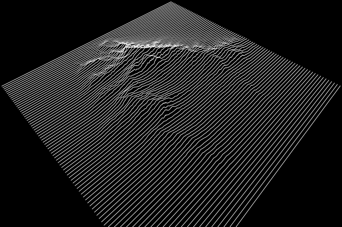 |
 |
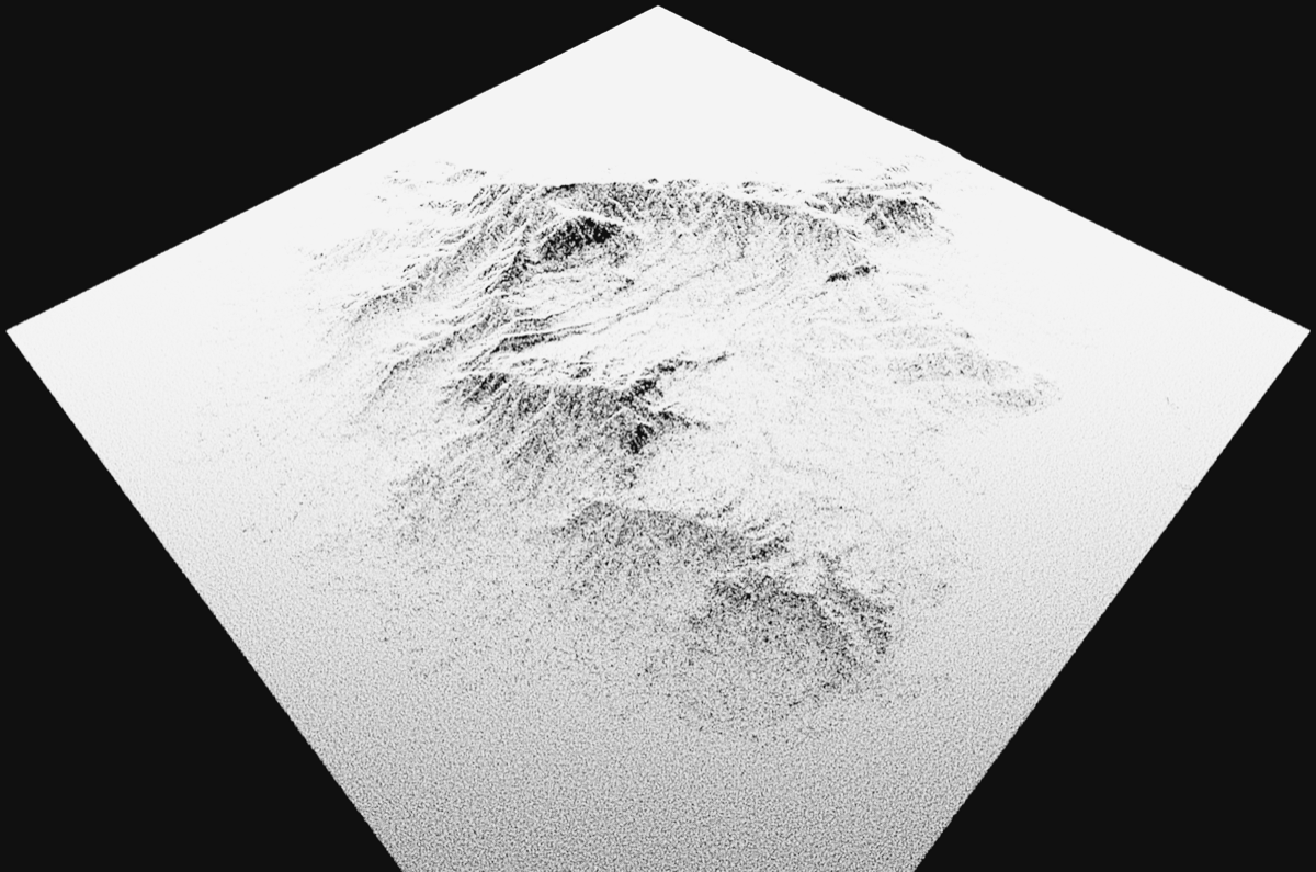 |
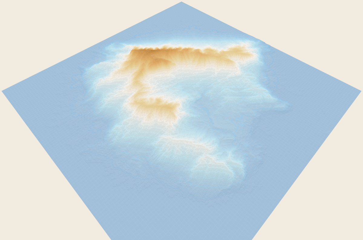
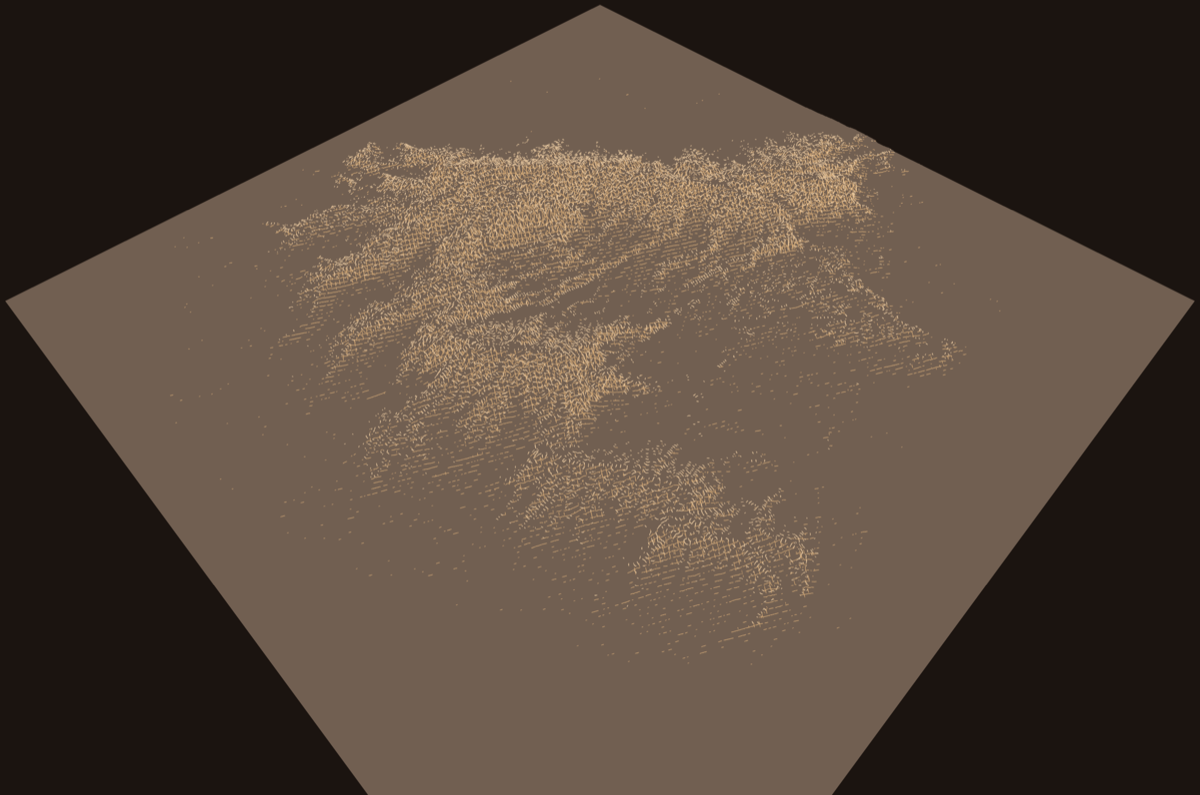
| Unknown Pleasures — stacked ridgelines | Alpine Survey — hypsometric fill, hillshade, contours | Static — slope-inverted stipple dots |
 |
 |
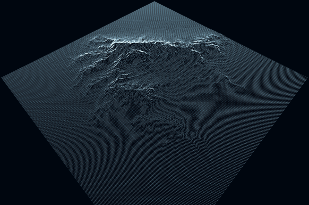 |
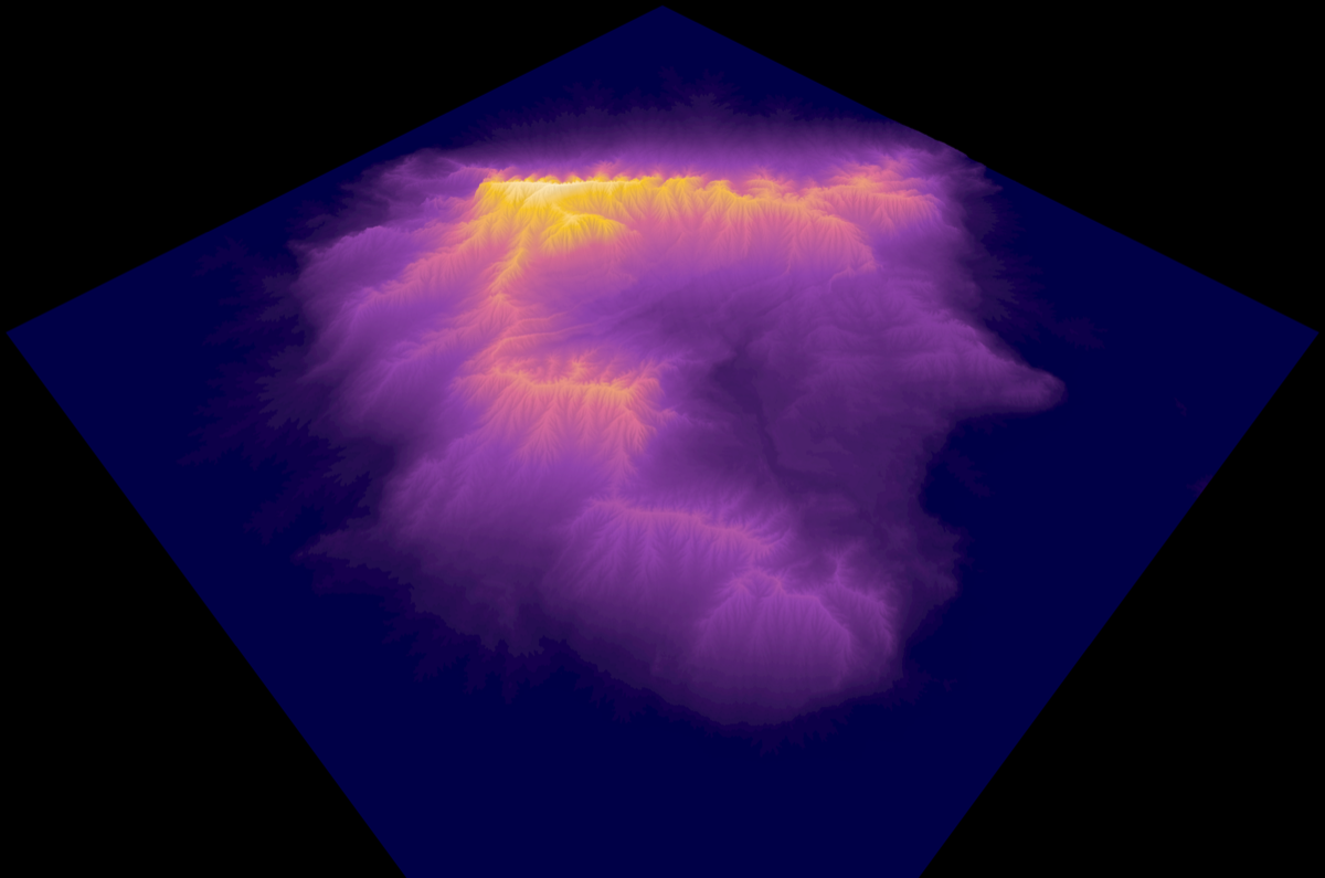
| Thermal Camera — hypsometric fill + sky-view AO | Copper Plate — curvature engraving | X-Ray — lines and crosshatch, ghost-occluded |
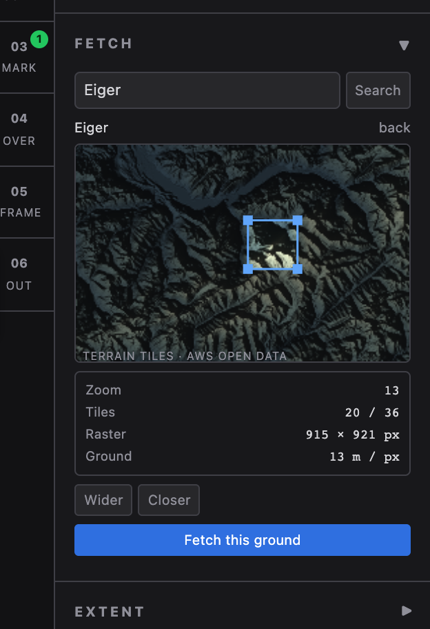 A smaller Fetch box gives a sharper raster, not a smaller file. The zoom is
always the finest that fits the 36-tile budget.
**Drag and drop.** Drop a file anywhere on the window. The app routes it by its
content, not by guess:
- A GeoTIFF becomes the terrain.
- A GPX or GeoJSON becomes an overlay.
- A cover plate becomes the land cover.
- A preset JSON, or a PNG or SVG that this app exported, restores the look.
A PNG with the app's `tEXt` chunk is a preset. A PNG without it is terrain.
**Vector layers.** OpenStreetMap data arrives as one layer per tag class, for
example *Roads · Motorway* or *Water · Stream*. Each layer has its own colour,
weight, opacity, dash and optional slope-following fill. The list is a stack:
drag a row to change what covers what. Inside a layer, each feature has a
checkbox. Rest the pointer on a feature to name it and light it up.
A point feature can carry its **name and height as labels**, in Space Mono or in
one of 49 **single-line fonts** (Hershey, EMS, Relief SingleLine, ISO 3098 and
three plotter faces). A stroke face plots each letter as centre lines, so the
label layer of the SVG is about a quarter of the size. The SVG writes real
`
A smaller Fetch box gives a sharper raster, not a smaller file. The zoom is
always the finest that fits the 36-tile budget.
**Drag and drop.** Drop a file anywhere on the window. The app routes it by its
content, not by guess:
- A GeoTIFF becomes the terrain.
- A GPX or GeoJSON becomes an overlay.
- A cover plate becomes the land cover.
- A preset JSON, or a PNG or SVG that this app exported, restores the look.
A PNG with the app's `tEXt` chunk is a preset. A PNG without it is terrain.
**Vector layers.** OpenStreetMap data arrives as one layer per tag class, for
example *Roads · Motorway* or *Water · Stream*. Each layer has its own colour,
weight, opacity, dash and optional slope-following fill. The list is a stack:
drag a row to change what covers what. Inside a layer, each feature has a
checkbox. Rest the pointer on a feature to name it and light it up.
A point feature can carry its **name and height as labels**, in Space Mono or in
one of 49 **single-line fonts** (Hershey, EMS, Relief SingleLine, ISO 3098 and
three plotter faces). A stroke face plots each letter as centre lines, so the
label layer of the SVG is about a quarter of the size. The SVG writes real
`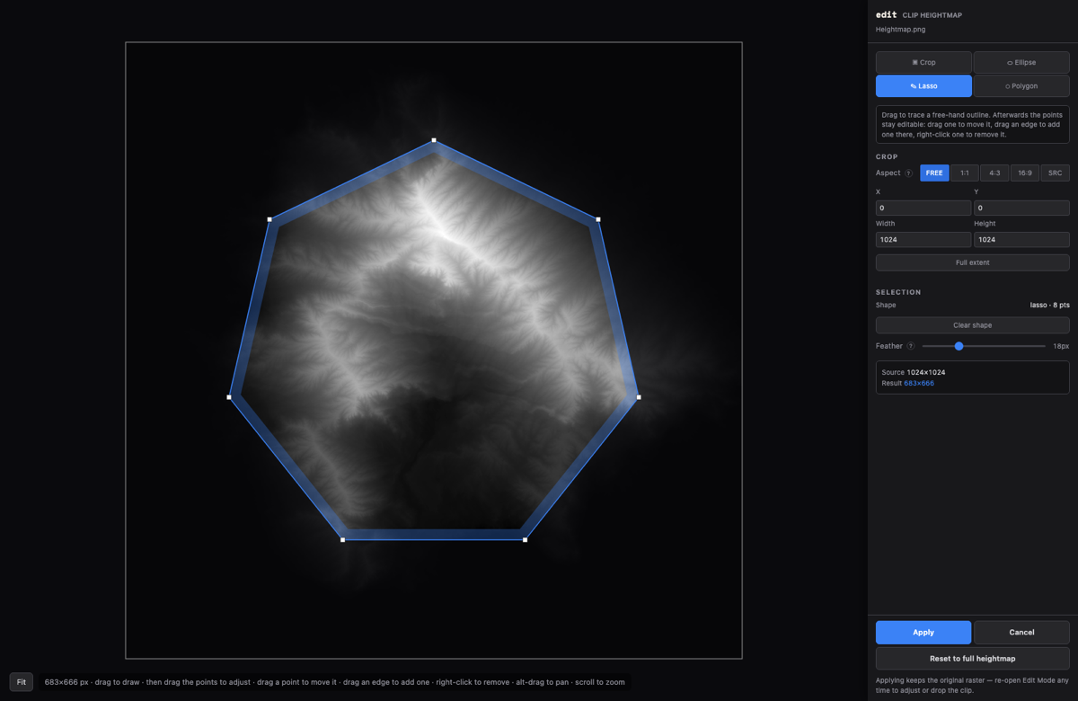 Press `E`. The viewport shows the raster flat. Crop it with a rectangle, an
ellipse, a lasso or a polygon, or clip it to a feature from a loaded layer, for
example a municipality or a lake.
- `C`, `O`, `L`, `P` and `F` pick Crop, Ellipse, Lasso, Polygon and Features.
The Features tool shows the outline before you clip.
- Drag a point to move it. Drag an edge to add a point. Right-click a point to
remove it.
- `⌘Z` undoes a change to the clip. Cancel discards the whole draft.
- *Feather* ramps the clipped edge down to the base level.
- The clip is non-destructive. Enter Edit Mode again to change it, or clear it.
Edit Mode works on a PNG, a GeoTIFF and a Soundscape. A GeoTIFF bounding box is
re-derived for the crop, so vector layers stay in place. Every draw mode stops
at the cut. → [Edit Mode](docs/Edit-Mode.md)
---
## Draw modes
Every mode runs independently, with its own colour, weight, line style (solid,
dashed, short, long or round dots) and colour: the line colour, a gradient by
height, slope or aspect, or the land cover class. Each mode also sets whether it
is an occluder, and a halo that breaks the lines behind it.
→ [Draw mode mathematics](docs/Draw-Modes.md) · [Occlusion](docs/Draw-Modes.md#occlusion)
**Duplicate this mode**, in the Copies block at the foot of a mode's section, adds a copy of the mode with
its own settings, mask and pens: for example, dense contours on forest and
sparse ones on rock. → [Copies](docs/Draw-Modes.md#copies)
| Mode | Technique |
|---|---|
| Lines | Parallel terrain ridgelines at any bearing |
| Crosshatch | Two perpendicular line sets at a set angle, with optional plus signs at the intersections as their own pen |
| Pillars | Vertical extrusion per cell (line, cuboid or cylinder), below and optionally above the ground, inked by land cover class |
| Contours | Marching Squares isolines, with optional ring closing and Chaikin smoothing |
| Hachure | Slope-directed short strokes, or Lehmann downslope strokes between contours |
| Flow Lines | Euler-integrated drainage paths |
| Stream Network | Strahler-order network, optionally weighted by flow accumulation |
| Pencil Shading | Laplacian curvature |
| Ridge Detection | Hessian eigenvalue crests |
| Valley Detection | Topographic Position Index troughs |
| Stipple Dots | Stochastic dot density from slope or elevation |
| Isophotes | Lines of constant illumination |
| Shadow Line | The shadow edge at one date, time and zone |
| Sun Hours | Isolines of hours in direct sun, over a year or one date |
| Engraving | Copperplate cross-hatch, up to 4 stacked directions |
| Curvature | Streamlines through the principal-curvature field |
| Rock & Scree | Swisstopo-style cliff hachures and scree dots |
| Bitplane | Marching squares without interpolation, with a Bayer screen |
| Sprite Blocks | The same quantiser drawn as blocks |
| Flashbulb | A point light in the scene with 1/r² falloff and a cast shadow |
| Halation | Blown highlights that bleed into the shadow beside them |
| Reticulation | Worley cell walls thinned by tone |
| Fall Line | Descent with mass: it overshoots, banks and runs out |
| Berms | Lateral load on the outside of each turn |
| Air | Spans where the ballistic path clears the surface |
| Race Line | All lines from one drop-in, the fastest inked heavier |
| Crossings | Sign changes of the detrended scanline |
| Indexed | Elevation tier by slope class, Bayer-dithered |
| Outrun | An additive halo under a near-white filament |
| Riso | Three spot inks screened at 15°, 45° and 75°, multiplied |
| Mineral | Five materials by slope and curvature, each with its own grain |
| Landforms | Ten landforms by geomorphons (peak, ridge, spur, hollow, valley …), one ink each. Every mode can also draw only on chosen landforms, or take its colour from them |
| Land cover | The classes of a loaded cover plate |
| Watershed | One flat ink per catchment |
| Single Line | One travelling-salesman tour through a weighted stipple |
| Shadow Hatch | Cross-hatching only inside cast and attached shadow |
| Roughness Mesh | Delaunay or Voronoi net, dense where the ground is rugged |
| Isochrones | Lines of equal walking time from one point (Tobler's hiking function) |
| Truchet | Quarter-arc tiles turned to follow the slope |
| Viewshed | The ground visible from one point, hatched |
| Route | The fastest walk between two points, with its time |
| Panorama | The ridges seen from one point, each where it hides the ground behind it, and the skyline |
| Bedding | Where tilted layers of rock crop out, for a dip and a dip direction, with a marker bed |
| Slope Classes | The avalanche map's bands, 30–35°, 35–40° and over 40°, one hatch and one pen each |
| Wind | Streamlines of one wind, bent along the slopes, crowded on the crests, broken in the lee |
| Runout | Where falling rock stops, by the reach angle of hazard maps, with the release zones |
| Venation | Leaf veins grown up the wet ground from the outlets (space colonization) |
| Geodesic Fan | Straight lines on the ground from one point, bent round the mountains |
| Radar | A side-looking radar's view as range ticks, with layover and radar shadow |
| Spines | The skeleton of the ground above each of a stack of levels |
| Coral | One closed line grown by differential growth until it fills the high ground |
| Glacier | Ice above a snowline, with blue contours, crevasses and moraine |
| Map Grid | A grid at a round true distance from the south-west corner, as lines or crosses, with the map sheet's edge scale in km |
| Line Printer | A SYMAP line-printer map: one glyph per character cell, from a dot to an overprinted block |
| Stems | A dotted stem from a datum to the ground at each cell, with a dot at the tip |
| Hair | A short curling stroke at each cell; seen from the side, the overlap is the tone |
| Waveform | A column of scanlines read along a line through the summit, the middle or a picked point, at any direction, mirrored or one-sided, as on a record sleeve. The line shows on the terrain while its section is open |
| Profile Sheet | A surveyor's profile sheet: parallel transects as rising profiles over a numbered station rule at every bend, with a band of cross profiles |
| Swath Profile | The mean, highest and lowest height across a strip along the plate, the envelope hatched, in metres and kilometres |
| Hypsometry | Strahler's hypsometric curve, with its histogram and the hypsometric integral |
| Aspect Rose | A rose diagram of the way the ground faces, weighted by slope, on an equal-area scale |
| Stereonet | Every slope's pole on a lower-hemisphere equal-area net, with density contours |
Indexed, Mineral, Land cover and Watershed export as closed filled paths, one
pen layer per ink. Set *Filled areas in the SVG* to Hatch (Output) and each
fill becomes hatch strokes a pen can draw, denser for darker inks.
**Occlusion.** Under *Occluder: Lines*, the default, each stroke hangs an
invisible wall down to the base, so lines hide other lines: the classic
ridgeline look. Each mode can stop being an occluder, and marks such as Hachure
start that way. Under *Occluder: Ground*, the terrain hides what is behind it,
with or without a fill. A mode's *Halo* breaks the lines behind its strokes.
*Stroke depth bias* keeps strokes on steep slopes at full width in front of the
terrain. Hidden segments can take their own colour and opacity.
**Inks as picked.** By default inks pass through a filmic tone curve and look
softer on screen. Switch this on in Terrain Style to draw and export every ink
exactly as picked, so a pen matched to a swatch matches the plot.
**Plan oblique.** A straight-down view in which each point moves up the sheet
by its height (Jenny and Patterson, 2007), so the mountains stand up while the
ground keeps its true shape and scale. It is in the Camera section, and the PNG
and SVG follow it.
**Anaglyph.** Every layer is drawn twice with a real parallax offset, for
red/cyan glasses. Filled areas take the eye's ink too, with their tone as its
weight. The SVG writes each eye as its own pen layer.
**Text layers.** Place your own words on the plate, in any label font. Each text
is its own layer and pen, and follows the ground under it.
**Presets.** 65 presets ship as thumbnails. *Surprise me* rolls a seeded look:
one to three modes, a palette and at most one overlay, with an ink that shows
against the background. It skips modes that need a file, a picked point, a date
or a georeference. ↩ and ↪ step through the last 50 seeds of the session.
**Seeds.** Stipple, Rock & Scree, Flashbulb, Halation, Reticulation, Single Line
and Roughness Mesh carry a seed. The same seed gives the same pattern.
---
## Surface overlays
- **Hillshade** with ray-marched cast shadows. Set darkness, softness and
quality. Multi-directional mode blends several azimuths.
- **Local light**, as in Swiss hand shading: the light turns at each place to
cross the ridges, so a ridge that runs along the light still has a lit and a
shaded flank.
- **Almanac sun.** Set a date, time and zone. The app computes the real solar
position from the raster's latitude and states sunrise, noon and sunset.
- **Slope shading** in true degrees, smooth or in bands, and a bivariate
**aspect map** that fades to grey on flat ground.
- **Sky-view factor** occlusion, and **openness** as grey or as a Red Relief
Image Map (slope in red).
- **Local relief** (the ground minus a blur of itself) and **curvature**
shading, for form without a light direction.
- **Texture shading** after Leland Brown: the ridge and gully network at every
scale, from a fractional Laplacian of the ground.
- **Aerial perspective**: low ground fades into haze.
- **Wetness** (the topographic wetness index) and **sunlight** (hours of direct
sun over a year or one day) as tints.
- **Water fill** at a set level, and **Tanaka** contours.
- **Hypsometric tinting** from a shared editable gradient.
- **Texture overlay** with blend modes, scale and offset.
## Terrain tools
- **Raw terrain view** shows the processed heightmap as a flat greyscale plane.
It costs no rebuild.
- **Levels** sets black and white points over a live histogram, with elevation
cuts.
- **Hydraulic erosion** runs a droplet simulation in a worker, after
[Hans Beyer's method](https://ardordeosis.github.io/implementation-of-a-method-for-hydraulic-erosion/thesis-beyer.pdf).
→ [Hydraulic erosion](docs/Hydraulic-Erosion.md)
- **Mirror** reflects the raster on X or Y.
- **Analysis** draws an elevation profile between two clicked points and marks
the cut on the terrain. The profile exports as its own SVG.
- **Hologram particles** animate a point cloud entirely in the vertex shader.
- **Murmurations** fly up to 100 000 boids over the terrain. Each bird follows
its eight nearest neighbours, as real starlings do. Birds roost on the highest
peak, ride updrafts, flee an optional predator and cast shadows. Drop an MP3
on the Particles panel and the flock reacts to it. `Space` pauses, and the SVG
export draws the frozen frame. → [Murmurations](docs/Murmurations.md)
## Soundscapes
Upload a track and it becomes terrain. A worker analyses the audio once into a
spectrogram (radix-2 FFT, Hann-windowed STFT, 75% overlap). Playback streams a
scrolling window of it into the raster slot, so every mode and exporter works
unchanged. Click the spectrogram to seek.
*Freeze Whole Track* writes the whole track as one heightmap, in five shapes:
stretched spectrogram, **Disc**, **Similarity** matrix, **Weave** on the bar
grid, and **Strata**. → [Soundscapes](docs/Soundscapes.md)
---
## Export
| Format | Notes |
|---|---|
| **SVG** | Software Z-buffer with terrain occlusion. One Inkscape layer per mode and per vector layer. Exact dash patterns. Shows progress and can be cancelled. |
| **PNG** | 4K with MSAA, trimmed to content. **PNG α** has a transparent background. |
| **STL** | Watertight mesh. A vector layer with **STL ribbon** gets a second solid for multicolour printing. |
| **Heightmap PNG** | The processed greyscale raster. |
| **WebM** | A recording of the live canvas. |
| **Profile SVG** | The elevation profile as a chart. |
Exports take the source file name: `graz.tif` gives `graz.svg`, `graz.png`,
`graz-alpha.png`, `graz.stl` and so on.
- **Every plate is a preset.** A PNG carries the parameters in a `tEXt` chunk,
an SVG in a comment. Open the file with *Preset ⬆* to restore the look. The
raster and its file name are never written.
- **Paper frame.** ISO A, US sizes, common ratios or your own, with a margin.
The SVG is cut at the frame, not clipped.
- **Scale bar and north arrow**, measured from the raster's bounding box. With a
sheet width in mm, the panel prints the map ratio.
- **Preflight** reports the stroke count, pen count, ink length, pen-up travel
and an estimated plot time.
- **Plotter order** re-orders strokes inside each pen layer. On the sample plate
it cuts pen-up travel from 52.4 m to 1.4 m. It is off by default, because
stroke order decides which ink is on top.
- **Command line.** `node scripts/erzberg.js render graz.tif -p Blueprint -o
graz.svg` renders a plate without the panel, through the same app in headless
Chrome. Draw modes, presets and any parameter are arguments.
→ [Command line](docs/CLI.md)
---
## Keyboard
| Key | Action |
|---|---|
| `E` | Enter Edit Mode |
| `Esc` | Cancel the current shape, leave Edit Mode, or cancel a profile pick |
| `Enter` | Close the current shape, or apply the clip |
| `Backspace` | Remove the last polygon vertex |
| `C` `O` `L` `P` `F` | Edit Mode tools |
| `Shift` | Constrain an ellipse to a circle |
| Right-click | Remove a point from a lasso or polygon |
| `Q` | Toggle auto-rotate |
| `Space` | Freeze the particle field |
| `\` | Show or hide the panel |
| `/` | Find a control |
| `1` – `5` | Export SVG, PNG, PNG α, STL, WebM |
| `⌘Z` / `Ctrl+Z` | Undo |
| `⌘⇧Z` / `Ctrl+Y` | Redo |
| `?` | Show this table in the app |
Shortcuts are bare keys, so browser chords pass through. Undo is the exception.
Inside a text box, `⌘Z` belongs to the browser. A slider drag is one undo step.
---
## Performance
- **On-demand rendering.** The canvas draws only when something changes.
- **Camera on the fast path.** Orbit moves the camera directly. React state
follows on a throttled tick. A production build holds 241 frames in 4 s with
p95 17.6 ms.
- **Off-thread geometry.** A long-lived worker rebuilds geometry and returns it
zero-copy, with normals and bounding spheres, so the main thread does not walk
the vertices. The worker caches the raster, so a slider move sends only
parameters.
- **Coalesced rebuilds.** Fast requests queue on a newest-wins rule.
- **Only what is seen.** Visual controls never rebuild. Normals, curtains and
the ray-march texture are built only when something uses them.
- **Supersampling** up to 2× device pixel ratio calms hairline shimmer.
---
## Tech stack
| Layer | Library |
|---|---|
| 3D engine | React Three Fiber + Three.js |
| State | Zustand (raster data) + React state (parameters), saved to `localStorage` |
| GIS | GeoTIFF.js, plus in-house GeoJSON, GPX and Overpass readers |
| Icons | Maki (CC0) |
| Fonts | Space Mono for the wordmark and labels, Overpass and Overpass Mono for the panel (all SIL OFL 1.1), self-hosted. 49 stroke faces from [oskay/svg-fonts](https://gitlab.com/oskay/svg-fonts), [Relief SingleLine](https://github.com/isdat-type/Relief-SingleLine), ISO 3098 and three plotter faces |
| Map data | OpenStreetMap through Overpass and Nominatim (ODbL) |
| Elevation | Terrain Tiles on AWS Open Data (SRTM, GMTED2010, EU-DEM, 3DEP) |
| Solar position | NOAA polynomials, in-house |
| UI | Custom panel + Tailwind CSS |
| Workers | Geometry, erosion, spectrogram |
| Audio | Web Audio + an in-house radix-2 FFT |
| Tests | Vitest (pure maths) and Playwright (headless Chrome, live dev server) |
---
## Documentation
- [Architecture: how a file becomes a picture](docs/Architecture.md)
- [Command line](docs/CLI.md)
- [Draw mode mathematics](docs/Draw-Modes.md)
- [Edit Mode](docs/Edit-Mode.md)
- [Georeferencing](docs/Georeferencing.md)
- [Hydraulic erosion](docs/Hydraulic-Erosion.md)
- [Land cover](docs/Land-Cover.md)
- [Masks and satellite imagery](docs/Masks.md)
- [Murmurations](docs/Murmurations.md)
- [Soundscapes](docs/Soundscapes.md)
- [Changelog](CHANGELOG.md)
---
## Development
```bash
npm install
npm run dev # dev server at http://localhost:5173
npm run build # production build + dist/THIRD-PARTY-NOTICES.txt
npm run lint # ESLint, correctness rules only
npm run test:unit # Vitest, the pure maths
npm run test # Playwright, both halves, headless
npm run test:light # specs that do not touch the GPU, 4 workers
npm run test:heavy # specs that do, 1 worker
HEADED=1 npm run test # with a visible window
npm run test:ui # Playwright interactive UI
npx playwright test tests/lines.spec.js # one spec
npm run update-presets # round-trip all presets through the live app
npm run thumbs # regenerate the preset thumbnails
npm run fonts:single-line # refetch and flatten the stroke faces
npm run licenses # regenerate the third-party notices
npm run logo # flatten
Press `E`. The viewport shows the raster flat. Crop it with a rectangle, an
ellipse, a lasso or a polygon, or clip it to a feature from a loaded layer, for
example a municipality or a lake.
- `C`, `O`, `L`, `P` and `F` pick Crop, Ellipse, Lasso, Polygon and Features.
The Features tool shows the outline before you clip.
- Drag a point to move it. Drag an edge to add a point. Right-click a point to
remove it.
- `⌘Z` undoes a change to the clip. Cancel discards the whole draft.
- *Feather* ramps the clipped edge down to the base level.
- The clip is non-destructive. Enter Edit Mode again to change it, or clear it.
Edit Mode works on a PNG, a GeoTIFF and a Soundscape. A GeoTIFF bounding box is
re-derived for the crop, so vector layers stay in place. Every draw mode stops
at the cut. → [Edit Mode](docs/Edit-Mode.md)
---
## Draw modes
Every mode runs independently, with its own colour, weight, line style (solid,
dashed, short, long or round dots) and colour: the line colour, a gradient by
height, slope or aspect, or the land cover class. Each mode also sets whether it
is an occluder, and a halo that breaks the lines behind it.
→ [Draw mode mathematics](docs/Draw-Modes.md) · [Occlusion](docs/Draw-Modes.md#occlusion)
**Duplicate this mode**, in the Copies block at the foot of a mode's section, adds a copy of the mode with
its own settings, mask and pens: for example, dense contours on forest and
sparse ones on rock. → [Copies](docs/Draw-Modes.md#copies)
| Mode | Technique |
|---|---|
| Lines | Parallel terrain ridgelines at any bearing |
| Crosshatch | Two perpendicular line sets at a set angle, with optional plus signs at the intersections as their own pen |
| Pillars | Vertical extrusion per cell (line, cuboid or cylinder), below and optionally above the ground, inked by land cover class |
| Contours | Marching Squares isolines, with optional ring closing and Chaikin smoothing |
| Hachure | Slope-directed short strokes, or Lehmann downslope strokes between contours |
| Flow Lines | Euler-integrated drainage paths |
| Stream Network | Strahler-order network, optionally weighted by flow accumulation |
| Pencil Shading | Laplacian curvature |
| Ridge Detection | Hessian eigenvalue crests |
| Valley Detection | Topographic Position Index troughs |
| Stipple Dots | Stochastic dot density from slope or elevation |
| Isophotes | Lines of constant illumination |
| Shadow Line | The shadow edge at one date, time and zone |
| Sun Hours | Isolines of hours in direct sun, over a year or one date |
| Engraving | Copperplate cross-hatch, up to 4 stacked directions |
| Curvature | Streamlines through the principal-curvature field |
| Rock & Scree | Swisstopo-style cliff hachures and scree dots |
| Bitplane | Marching squares without interpolation, with a Bayer screen |
| Sprite Blocks | The same quantiser drawn as blocks |
| Flashbulb | A point light in the scene with 1/r² falloff and a cast shadow |
| Halation | Blown highlights that bleed into the shadow beside them |
| Reticulation | Worley cell walls thinned by tone |
| Fall Line | Descent with mass: it overshoots, banks and runs out |
| Berms | Lateral load on the outside of each turn |
| Air | Spans where the ballistic path clears the surface |
| Race Line | All lines from one drop-in, the fastest inked heavier |
| Crossings | Sign changes of the detrended scanline |
| Indexed | Elevation tier by slope class, Bayer-dithered |
| Outrun | An additive halo under a near-white filament |
| Riso | Three spot inks screened at 15°, 45° and 75°, multiplied |
| Mineral | Five materials by slope and curvature, each with its own grain |
| Landforms | Ten landforms by geomorphons (peak, ridge, spur, hollow, valley …), one ink each. Every mode can also draw only on chosen landforms, or take its colour from them |
| Land cover | The classes of a loaded cover plate |
| Watershed | One flat ink per catchment |
| Single Line | One travelling-salesman tour through a weighted stipple |
| Shadow Hatch | Cross-hatching only inside cast and attached shadow |
| Roughness Mesh | Delaunay or Voronoi net, dense where the ground is rugged |
| Isochrones | Lines of equal walking time from one point (Tobler's hiking function) |
| Truchet | Quarter-arc tiles turned to follow the slope |
| Viewshed | The ground visible from one point, hatched |
| Route | The fastest walk between two points, with its time |
| Panorama | The ridges seen from one point, each where it hides the ground behind it, and the skyline |
| Bedding | Where tilted layers of rock crop out, for a dip and a dip direction, with a marker bed |
| Slope Classes | The avalanche map's bands, 30–35°, 35–40° and over 40°, one hatch and one pen each |
| Wind | Streamlines of one wind, bent along the slopes, crowded on the crests, broken in the lee |
| Runout | Where falling rock stops, by the reach angle of hazard maps, with the release zones |
| Venation | Leaf veins grown up the wet ground from the outlets (space colonization) |
| Geodesic Fan | Straight lines on the ground from one point, bent round the mountains |
| Radar | A side-looking radar's view as range ticks, with layover and radar shadow |
| Spines | The skeleton of the ground above each of a stack of levels |
| Coral | One closed line grown by differential growth until it fills the high ground |
| Glacier | Ice above a snowline, with blue contours, crevasses and moraine |
| Map Grid | A grid at a round true distance from the south-west corner, as lines or crosses, with the map sheet's edge scale in km |
| Line Printer | A SYMAP line-printer map: one glyph per character cell, from a dot to an overprinted block |
| Stems | A dotted stem from a datum to the ground at each cell, with a dot at the tip |
| Hair | A short curling stroke at each cell; seen from the side, the overlap is the tone |
| Waveform | A column of scanlines read along a line through the summit, the middle or a picked point, at any direction, mirrored or one-sided, as on a record sleeve. The line shows on the terrain while its section is open |
| Profile Sheet | A surveyor's profile sheet: parallel transects as rising profiles over a numbered station rule at every bend, with a band of cross profiles |
| Swath Profile | The mean, highest and lowest height across a strip along the plate, the envelope hatched, in metres and kilometres |
| Hypsometry | Strahler's hypsometric curve, with its histogram and the hypsometric integral |
| Aspect Rose | A rose diagram of the way the ground faces, weighted by slope, on an equal-area scale |
| Stereonet | Every slope's pole on a lower-hemisphere equal-area net, with density contours |
Indexed, Mineral, Land cover and Watershed export as closed filled paths, one
pen layer per ink. Set *Filled areas in the SVG* to Hatch (Output) and each
fill becomes hatch strokes a pen can draw, denser for darker inks.
**Occlusion.** Under *Occluder: Lines*, the default, each stroke hangs an
invisible wall down to the base, so lines hide other lines: the classic
ridgeline look. Each mode can stop being an occluder, and marks such as Hachure
start that way. Under *Occluder: Ground*, the terrain hides what is behind it,
with or without a fill. A mode's *Halo* breaks the lines behind its strokes.
*Stroke depth bias* keeps strokes on steep slopes at full width in front of the
terrain. Hidden segments can take their own colour and opacity.
**Inks as picked.** By default inks pass through a filmic tone curve and look
softer on screen. Switch this on in Terrain Style to draw and export every ink
exactly as picked, so a pen matched to a swatch matches the plot.
**Plan oblique.** A straight-down view in which each point moves up the sheet
by its height (Jenny and Patterson, 2007), so the mountains stand up while the
ground keeps its true shape and scale. It is in the Camera section, and the PNG
and SVG follow it.
**Anaglyph.** Every layer is drawn twice with a real parallax offset, for
red/cyan glasses. Filled areas take the eye's ink too, with their tone as its
weight. The SVG writes each eye as its own pen layer.
**Text layers.** Place your own words on the plate, in any label font. Each text
is its own layer and pen, and follows the ground under it.
**Presets.** 65 presets ship as thumbnails. *Surprise me* rolls a seeded look:
one to three modes, a palette and at most one overlay, with an ink that shows
against the background. It skips modes that need a file, a picked point, a date
or a georeference. ↩ and ↪ step through the last 50 seeds of the session.
**Seeds.** Stipple, Rock & Scree, Flashbulb, Halation, Reticulation, Single Line
and Roughness Mesh carry a seed. The same seed gives the same pattern.
---
## Surface overlays
- **Hillshade** with ray-marched cast shadows. Set darkness, softness and
quality. Multi-directional mode blends several azimuths.
- **Local light**, as in Swiss hand shading: the light turns at each place to
cross the ridges, so a ridge that runs along the light still has a lit and a
shaded flank.
- **Almanac sun.** Set a date, time and zone. The app computes the real solar
position from the raster's latitude and states sunrise, noon and sunset.
- **Slope shading** in true degrees, smooth or in bands, and a bivariate
**aspect map** that fades to grey on flat ground.
- **Sky-view factor** occlusion, and **openness** as grey or as a Red Relief
Image Map (slope in red).
- **Local relief** (the ground minus a blur of itself) and **curvature**
shading, for form without a light direction.
- **Texture shading** after Leland Brown: the ridge and gully network at every
scale, from a fractional Laplacian of the ground.
- **Aerial perspective**: low ground fades into haze.
- **Wetness** (the topographic wetness index) and **sunlight** (hours of direct
sun over a year or one day) as tints.
- **Water fill** at a set level, and **Tanaka** contours.
- **Hypsometric tinting** from a shared editable gradient.
- **Texture overlay** with blend modes, scale and offset.
## Terrain tools
- **Raw terrain view** shows the processed heightmap as a flat greyscale plane.
It costs no rebuild.
- **Levels** sets black and white points over a live histogram, with elevation
cuts.
- **Hydraulic erosion** runs a droplet simulation in a worker, after
[Hans Beyer's method](https://ardordeosis.github.io/implementation-of-a-method-for-hydraulic-erosion/thesis-beyer.pdf).
→ [Hydraulic erosion](docs/Hydraulic-Erosion.md)
- **Mirror** reflects the raster on X or Y.
- **Analysis** draws an elevation profile between two clicked points and marks
the cut on the terrain. The profile exports as its own SVG.
- **Hologram particles** animate a point cloud entirely in the vertex shader.
- **Murmurations** fly up to 100 000 boids over the terrain. Each bird follows
its eight nearest neighbours, as real starlings do. Birds roost on the highest
peak, ride updrafts, flee an optional predator and cast shadows. Drop an MP3
on the Particles panel and the flock reacts to it. `Space` pauses, and the SVG
export draws the frozen frame. → [Murmurations](docs/Murmurations.md)
## Soundscapes
Upload a track and it becomes terrain. A worker analyses the audio once into a
spectrogram (radix-2 FFT, Hann-windowed STFT, 75% overlap). Playback streams a
scrolling window of it into the raster slot, so every mode and exporter works
unchanged. Click the spectrogram to seek.
*Freeze Whole Track* writes the whole track as one heightmap, in five shapes:
stretched spectrogram, **Disc**, **Similarity** matrix, **Weave** on the bar
grid, and **Strata**. → [Soundscapes](docs/Soundscapes.md)
---
## Export
| Format | Notes |
|---|---|
| **SVG** | Software Z-buffer with terrain occlusion. One Inkscape layer per mode and per vector layer. Exact dash patterns. Shows progress and can be cancelled. |
| **PNG** | 4K with MSAA, trimmed to content. **PNG α** has a transparent background. |
| **STL** | Watertight mesh. A vector layer with **STL ribbon** gets a second solid for multicolour printing. |
| **Heightmap PNG** | The processed greyscale raster. |
| **WebM** | A recording of the live canvas. |
| **Profile SVG** | The elevation profile as a chart. |
Exports take the source file name: `graz.tif` gives `graz.svg`, `graz.png`,
`graz-alpha.png`, `graz.stl` and so on.
- **Every plate is a preset.** A PNG carries the parameters in a `tEXt` chunk,
an SVG in a comment. Open the file with *Preset ⬆* to restore the look. The
raster and its file name are never written.
- **Paper frame.** ISO A, US sizes, common ratios or your own, with a margin.
The SVG is cut at the frame, not clipped.
- **Scale bar and north arrow**, measured from the raster's bounding box. With a
sheet width in mm, the panel prints the map ratio.
- **Preflight** reports the stroke count, pen count, ink length, pen-up travel
and an estimated plot time.
- **Plotter order** re-orders strokes inside each pen layer. On the sample plate
it cuts pen-up travel from 52.4 m to 1.4 m. It is off by default, because
stroke order decides which ink is on top.
- **Command line.** `node scripts/erzberg.js render graz.tif -p Blueprint -o
graz.svg` renders a plate without the panel, through the same app in headless
Chrome. Draw modes, presets and any parameter are arguments.
→ [Command line](docs/CLI.md)
---
## Keyboard
| Key | Action |
|---|---|
| `E` | Enter Edit Mode |
| `Esc` | Cancel the current shape, leave Edit Mode, or cancel a profile pick |
| `Enter` | Close the current shape, or apply the clip |
| `Backspace` | Remove the last polygon vertex |
| `C` `O` `L` `P` `F` | Edit Mode tools |
| `Shift` | Constrain an ellipse to a circle |
| Right-click | Remove a point from a lasso or polygon |
| `Q` | Toggle auto-rotate |
| `Space` | Freeze the particle field |
| `\` | Show or hide the panel |
| `/` | Find a control |
| `1` – `5` | Export SVG, PNG, PNG α, STL, WebM |
| `⌘Z` / `Ctrl+Z` | Undo |
| `⌘⇧Z` / `Ctrl+Y` | Redo |
| `?` | Show this table in the app |
Shortcuts are bare keys, so browser chords pass through. Undo is the exception.
Inside a text box, `⌘Z` belongs to the browser. A slider drag is one undo step.
---
## Performance
- **On-demand rendering.** The canvas draws only when something changes.
- **Camera on the fast path.** Orbit moves the camera directly. React state
follows on a throttled tick. A production build holds 241 frames in 4 s with
p95 17.6 ms.
- **Off-thread geometry.** A long-lived worker rebuilds geometry and returns it
zero-copy, with normals and bounding spheres, so the main thread does not walk
the vertices. The worker caches the raster, so a slider move sends only
parameters.
- **Coalesced rebuilds.** Fast requests queue on a newest-wins rule.
- **Only what is seen.** Visual controls never rebuild. Normals, curtains and
the ray-march texture are built only when something uses them.
- **Supersampling** up to 2× device pixel ratio calms hairline shimmer.
---
## Tech stack
| Layer | Library |
|---|---|
| 3D engine | React Three Fiber + Three.js |
| State | Zustand (raster data) + React state (parameters), saved to `localStorage` |
| GIS | GeoTIFF.js, plus in-house GeoJSON, GPX and Overpass readers |
| Icons | Maki (CC0) |
| Fonts | Space Mono for the wordmark and labels, Overpass and Overpass Mono for the panel (all SIL OFL 1.1), self-hosted. 49 stroke faces from [oskay/svg-fonts](https://gitlab.com/oskay/svg-fonts), [Relief SingleLine](https://github.com/isdat-type/Relief-SingleLine), ISO 3098 and three plotter faces |
| Map data | OpenStreetMap through Overpass and Nominatim (ODbL) |
| Elevation | Terrain Tiles on AWS Open Data (SRTM, GMTED2010, EU-DEM, 3DEP) |
| Solar position | NOAA polynomials, in-house |
| UI | Custom panel + Tailwind CSS |
| Workers | Geometry, erosion, spectrogram |
| Audio | Web Audio + an in-house radix-2 FFT |
| Tests | Vitest (pure maths) and Playwright (headless Chrome, live dev server) |
---
## Documentation
- [Architecture: how a file becomes a picture](docs/Architecture.md)
- [Command line](docs/CLI.md)
- [Draw mode mathematics](docs/Draw-Modes.md)
- [Edit Mode](docs/Edit-Mode.md)
- [Georeferencing](docs/Georeferencing.md)
- [Hydraulic erosion](docs/Hydraulic-Erosion.md)
- [Land cover](docs/Land-Cover.md)
- [Masks and satellite imagery](docs/Masks.md)
- [Murmurations](docs/Murmurations.md)
- [Soundscapes](docs/Soundscapes.md)
- [Changelog](CHANGELOG.md)
---
## Development
```bash
npm install
npm run dev # dev server at http://localhost:5173
npm run build # production build + dist/THIRD-PARTY-NOTICES.txt
npm run lint # ESLint, correctness rules only
npm run test:unit # Vitest, the pure maths
npm run test # Playwright, both halves, headless
npm run test:light # specs that do not touch the GPU, 4 workers
npm run test:heavy # specs that do, 1 worker
HEADED=1 npm run test # with a visible window
npm run test:ui # Playwright interactive UI
npx playwright test tests/lines.spec.js # one spec
npm run update-presets # round-trip all presets through the live app
npm run thumbs # regenerate the preset thumbnails
npm run fonts:single-line # refetch and flatten the stroke faces
npm run licenses # regenerate the third-party notices
npm run logo # flatten