---
title: "Reshaping, cleaning and tidying data"
author: "ENS-215"
date: "3-Feb-2025"
output:
  html_document:
    df_print: paged
    theme: journal
    toc: TRUE
    toc_float: TRUE
---

```{r echo=FALSE}
knitr::opts_chunk$set(comment=NA, warning = F)

```

<br/>

In most cases, the dataset that you want to work with will not be in an ideal format/structure for conducting your analysis.  In fact getting data into a suitable format and structure is often one of the more time consuming aspects of data analysis and interpretation.  Furthermore, a single format and structure typically will not suit all of your needs -- a given format/structure might work great for one aspect of your work, but be less than ideal (or completely unsuitable) for another task.  

Thankfully, there are many tools available in R that dramatically simplify the tasks of reshaping, cleaning, and tidying datasets.  These tools will allow you to prepare your data for the analysis you want to perform and will free up more of your time to focus on the scientific analysis and interpretation.  

Today and in the upcoming classes, we will start to work with tools from the `dplyr` and `tidyr` packages that allow you to efficiently deal with your data.  

While, you've been working with real, research quality datasets in class/lab, these datasets have been relatively neat and clean (In most cases I've taken the original dataset and done some organizing/cleaning to prepare it for the class).  However in most cases you won't have someone prep the data before you get it.  Thus, the skills you will now learn are critical to your work as they will allow you to deal with data "out in the real-world" where things can get a bit more messy.  


```{r message=FALSE, warning=F}
library(tidyverse)
```

<br/>

## Tidy data

In data science, **tidy** data has a specific meaning, and refers to how the data is organized within a data table.  The definition of tidy data that we will use in this class was nicely laid out by Wickham (author of R4DS):

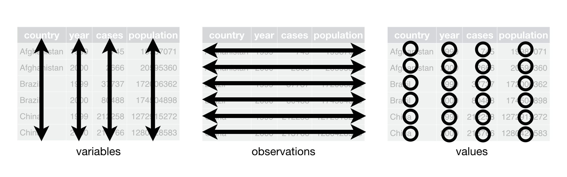
> A dataset is a collection of values, usually either numbers (if quantitative) or strings AKA text data (if qualitative). Values are organised in two ways. Every value belongs to a variable and an observation. A variable contains all values that measure the same underlying attribute (like height, temperature, duration) across units. An observation contains all values measured on the same unit (like a person, or a day, or a city) across attributes.  

>Tidy data is a standard way of mapping the meaning of a dataset to its structure. A dataset is messy or tidy depending on how rows, columns and tables are matched up with observations, variables and types. In tidy data:  

>1. Each **variable** forms a **column**  
2. Each **observation** forms a **row**  
3. Each type of observational unit forms a table.  

![_Image source: R4DS_](https://stahlm.github.io/ENS_215/Lectures/Images/tidy-1.png)

<br/>

In some cases, untidy data is more "human-readable".  Thus, you may receive data in untidy formats because it was originally formatted for human eyes to look at.  Other times you will receive untidy data, simply because the original formatter of the data wasn't thinking about (or didn't need to) these issues.  

When performing data analysis a tidy dataset is almost always much easier to work with and thus we will often convert untidy data into a tidy format (_however there are situations where an untidy dataset is useful_).  

<br/>

## Reshaping datasets

<br/>

### Reshape with `pivot_longer()`

Let's load in monthly precipitation (in inches) for Massachusetts for years 2015-2017.

```{r warning=FALSE, message=FALSE}
precip_untidy_MA <- read_csv("https://stahlm.github.io/ENS_215/Data/precip_untidy_MA.csv")
```


```{r warning=FALSE, message=FALSE, echo=FALSE}
library(kableExtra)

precip_untidy_MA %>% 
  kable() %>% 
  kable_styling(bootstrap_options = "condensed", position = "center") 

```


Take a look at the dataset  

+ How many columns are there? 
+ How many variables are there?  
+ How many rows are there?
+ How many observations are there? 

Based on what you found above, is the dataset in tidy format?  Explain what about the structure of the data allows you to know whether it is tidy or not.  

<br/> 

While the above data table is "human readable" it is not in the best format for most computing and data analysis operations due to the fact that it is untidy.  

We learned that in a tidy dataset each variable has its own column and each observation has its own row.  Our current dataset has 14 columns despite having only four variables (Year, Month, State, and precipitation in inches).  Furthermore our dataset has 3 rows, while having 36 observations (monthly observations for three years).  

Thus to make our dataset tidy, we will need to reshape the data so that we have four columns and 36 rows.  Three of the columns (Year, Month, State) are variables whose values identify the observation, while the fourth column will have the precipitation corresponding to a given observation.  


Ok, once you understand why the data isn't tidy, we'll move ahead and make it tidy.  To do this we will use the `pivot_longer()` function from the `tidyr` package.  

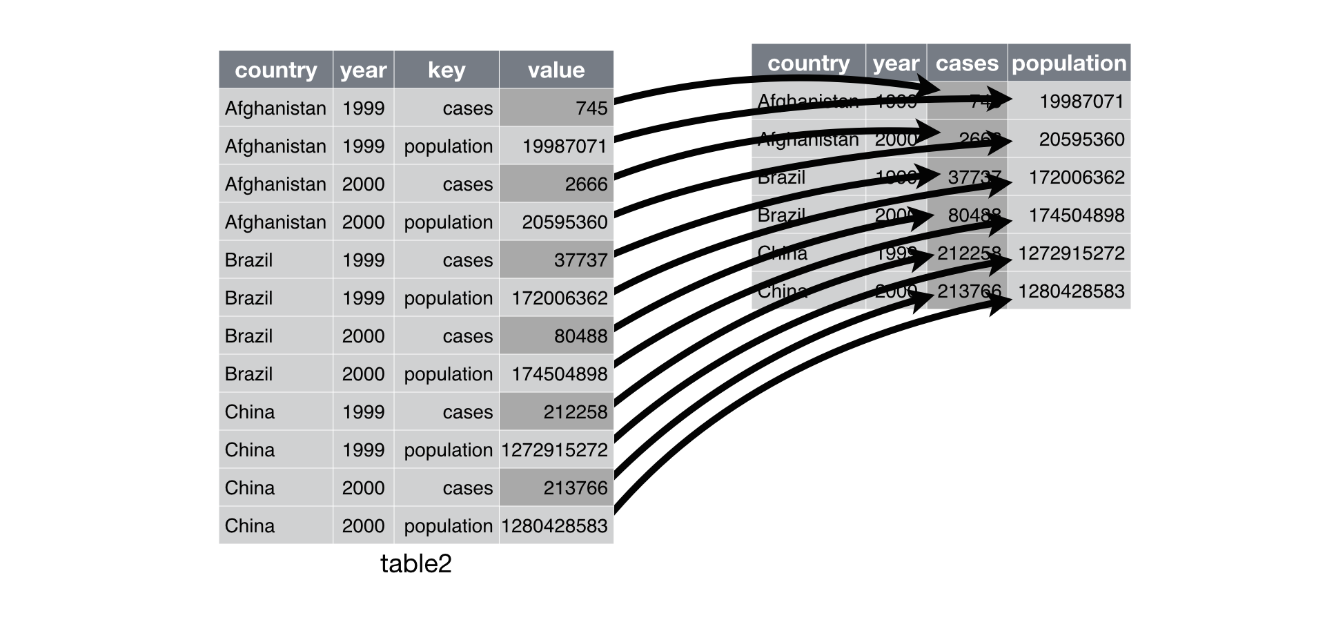
We can use the `pivot_longer` function to take the names of columns and gather them into a new column where the names are values in a variable.  For example, the above dataset has columns with month names, however these names are really values that should be in a variable (column) that has the months.  

Below is a nice illustration from the R4DS text that illustrates what `pivot_longer` does.  

![_Image source: R4DS_](https://stahlm.github.io/ENS_215/Lectures/Images/tidy-gather.png)

`pivot_longer()` takes four arguments:  

+ The dataset you would like to operate on  

+ **names_to**: This is the name of the new column that combines all column names from the original dataset (_i.e._ Jan, Feb, Mar,..., Dec) and stores them as data in this new column .  

+ **values_to**: This is the name of the new column that contains all values (_i.e._ precipitation values) associated with each variable combination (_i.e._ Jan 2015, Feb 2015,..., Dec 2017)  

+ **cols** This is a list of columns that are to be collapsed. The column can be referenced by column numbers or column names. 

In our case, the **names_to** will be called `Month`, the **values_to** will be called `Precip_inches`.  The **cols** will be the list of the columns that we want to gather (_i.e._ "Jan", "Feb",..., "Dec")  

To simplify things I am using the built in vector of month abbreviations `month.abb` in R, so that we don't have to type out a vector with the abbreviations of each month.  


```{r}
precip_tidy_MA <- precip_untidy_MA %>% 
  pivot_longer(cols = month.abb, names_to = "Month", values_to = "Precip_inches")
```


Take a look at the new data frame.  You'll see that each observation (defined by a unique State, Year, Month combination) has its own row.  Furthermore you'll see that we have one column with precipitation measurements, as opposed to the twelve columns of precip measurements that we had in untidy dataset.  

<br/>

### Reshape with `pivot_wider()`

In some cases you will encounter untidy data where there are too few columns in the original dataset, due to the fact that each variable has not been allocated its own column.  Let's load in a dataset that highlights this.  

```{r message=FALSE}
precip_temp_untidy_CA <- read_csv("https://stahlm.github.io/ENS_215/Data/CA_temp_precip_untidy.csv")

```


Take a look at the dataset and confirm that it is not in tidy format.
```{r}
precip_temp_untidy_CA
```

You can see that the `measurement_type` column specifies what kind of measurement is in the `measurement` column.  In our dataset the `measurment` column is holding values for two variables (precipitation and temperature).  Remember that a tidy dataset should have separate columns for each variable.  Thus we need to spread the values in `measurement` into two columns -- one for precipitation and one for temperature.  

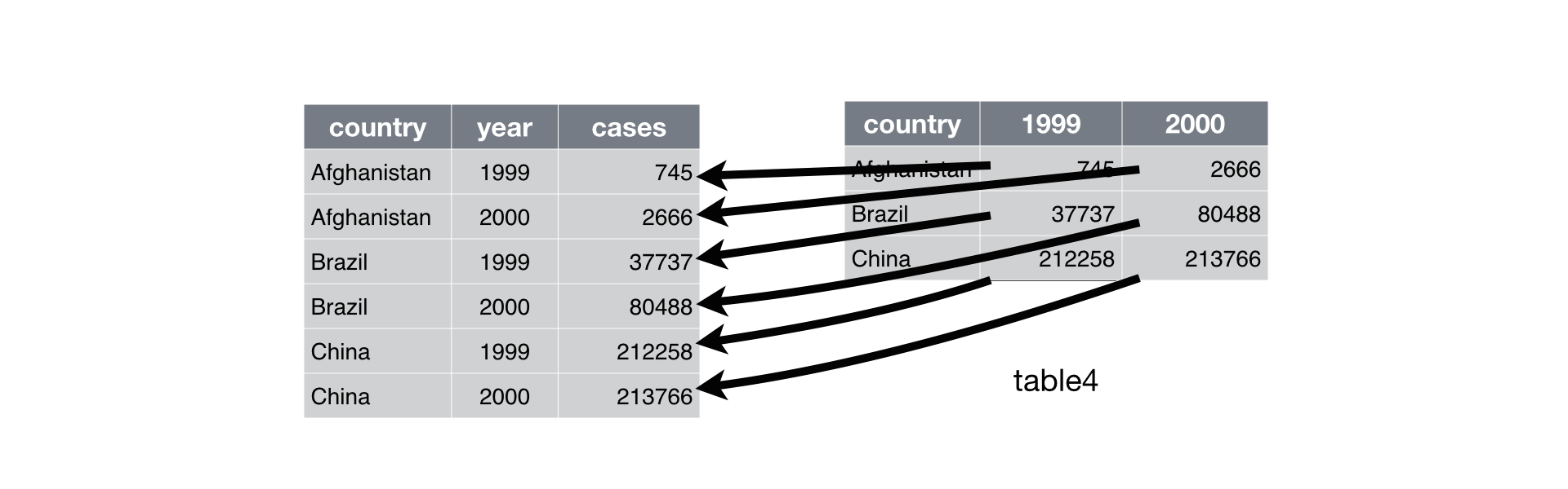
Below is a nice illustration from the R4DS text that illustrates what `pivot_wider()` does.  

![_Image source: R4DS_](https://stahlm.github.io/ENS_215/Lectures/Images/tidy-spread.png)

The `pivot_wider()` function can perform this operation.  `pivot_wider` takes three arguments:

+ The dataset to pivot wider  
+ **names_from:** The column in the original dataset that contains the names of the variables to spread into the new columns  
+ **values_from:** The column of the original dataset that contains the values that should be spread into the new columns  


Let's `pivot_wider()` our data to make it tidy.  Our **names_from** is the `measurement_type` and our **values_from** is the `measurement`

```{r}
# Your code here 
```

<br/>


```{r eval=FALSE, echo=FALSE}

precip_temp_tidy_CA <- precip_temp_untidy_CA %>% 
  pivot_wider(names_from = measurement_type, values_from = measurement)

precip_temp_tidy_CA
```

You can see that our tidy dataset has a single row for each observation (whereas the untidy data had two rows for each observation -- one for the precipitation and one for the temperature).  

<br/>

### Exercise

You've learned how to tidy data using `pivot_longer()` and `pivot_wider()`.  Let's get some more practice with these functions.  To do this let's undo our tidying.  There are situations where you might want untidy data, but the main reason we are doing this untidying here is to test your understanding of how to use `pivot_longer()` and `pivot_wider()`.  

1. Use `pivot_wider()` to untidy  `precip_tidy_MA` 
```{r eval=FALSE, echo=FALSE}

precip_tidy_MA %>%  
  pivot_wider(names_from = Month, values_from = Precip_inches)

```



2. Use `pivot_longer()` to untidy `precip_temp_tidy_CA`
```{r eval=FALSE, echo=FALSE}

precip_temp_tidy_CA %>% 
  pivot_longer(cols = c(Avg_Temp_F, Precip_inches), names_to = "Measurement_type", values_to = "Measurement")

```


<br/>

## "Cleaning" datasets
Just as the data that we come across in our work will often be untidy, so to will it often be "unclean".  By unclean, we mean that the data may have missing values or value formats that are not conducive to computing/data analysis.  Let's load in an example dataset containing information about the rivers with the highest flows. 

```{r message=FALSE}
Rivers_to_clean <- read_csv("https://stahlm.github.io/ENS_215/Data/Rivers_sep_unite.csv")
```

<br/>

There are four columns in the dataset:

+ Rank: rivers rank according to its flow (discharge)  
+ River: name of the river
+ Length_Drainage_Ratio: the ratio of the rivers length (km) to the area of the watershed (km^2^)
+ Discharge_m3_s: the average flow (discharge) in m^3^/s

Take a look at the data and you'll see that the dataset needs some cleaning.  In particular there is missing data `NA` in the `Discharge_m3_s` column and the `Length_Drainage_Ratio` is not in a very computable format.  

We'll learn a few helpful functions that allow us to quickly and easily clean up data.  

<br/>

### Remove rows with `NA`s using `drop_na()`
When you have `NA` values you may simply want to remove the rows containing the `NA`s, thus leaving you with a dataset that does not have any missing data.  This is often helpful, however you should always give thought to simply dropping observations that may have `NA`s in some of the columns as this can result in biases or oversight in your analysis.  

However, let's assume our analysis requires us to drop the rows with `NA`s.  To do this we use the `drop_na` function.  If you do not specify the columns to look in, then the `drop_na()` function will drop any rows that have `NA`s.  You can also pass the columns you would like `drop_na` to look in and it will only drop rows where the specified column(s) have `NA`s.  

```{r}
drop_na(Rivers_to_clean) # drop NAs (look at all columns)
```

<br/>

```{r}
drop_na(Rivers_to_clean, Rank) # drop NAs (look at Rank column)
```

You can see that the first example drops four rows, whereas the 2^nd^ example, which only looked in the `Rank` column didn't drop any rows, since `Rank` has no `NA` values.  

<br/>

### Deal with `NA`s using `replace_na()` and `fill()`
Sometimes we will want to replace `NA` values with a specified value.  

The `replace_na()` function allows us to replace missing data with a specified value
```{r}
replace_na(Rivers_to_clean, list(Discharge_m3_s = -9999)) # replace the missing discharge data with -9999
```

You can see that we replace the missing discharge data with another value.  In the `list()` function we can specify a list of columns and the values that we would like to replace `NA`s with in each of the columns.

<br/>

In some cases you may want to replace `NA`s by filling in the missing data with data in an adjacent row.  Since our data is ordered by rank, as a first guess, we could replace the missing discharge data with the value in the row above.  To do this type of operation we use the `fill()` function.  

<br/>

```{r}
Rivers_to_clean %>% 
  fill(Discharge_m3_s, .direction = "up")
```

You can fill from the row below (i.e. fill upwards) using `.direction = "up"`, or you can fill from the row above (i.e.) fill downwards using `.direction = "down"`.  Note that there is a period `.` before the direction.  

<br/>

### Separate values with `separate()` 
When you encounter data two values in a single cell you will typically want to separate them.  In the dataset we are working with the `Length_Drainage_Ratio` column has two values (river length and river watershed area) reported in each cell.  Let's separate these data into two separate columns.   To do this we'll use the `separate` function.  

```{r}
Rivers_to_clean <- Rivers_to_clean %>% 
  separate(col = Length_Drainage_Ratio, into = c("Length_km", "Area_km2"), sep = "/")

Rivers_to_clean 
```

You see that the `separate` function takes several arguments in addition to the dataset:  

+ col: column containing the values to separate  
+ into: a vector containing the names of the new columns to place the separated values  
+ sep: the character that indicates where the separation should be made  

<br/>

### Join values with `unite()`
In some cases you will have observations with values in two cells that you would like to combine into a single cell.  An example might be a dataset where you have the century in one column and the year in another and you would like to merge the two into a single year column.  To do this we would use the `unite` function.  

| Century 	| Year 	|
|---------	|------	|
| 20 	| 01 	|
| 20 	| 02 	|
| 20 	| 03 	|
| 20 	| 04 	|
| 20 	| 05 	|
| 20 	| 06 	|
| 20 	| 07 	|
| 20 	| 08 	|
| 20 	| 09 	|
| 20 	| 10 	|


Let's keep working with our River data though.  We can simply undo our separation that we performed earlier, just to highlight how to use the `unite` function.  

```{r}
Rivers_to_clean %>% 
  unite(Length_km, Area_km2, col = "Length_Area_Ratio", sep = "/")
```


<br/>


### Excercise
Now you've learned some important concepts regarding clean and tidy data along with some tools/techniques to help you clean and tidy your data and get it ready for analysis.  

#### **Examine the data**
Let's load in a file that has groundwater geochemistry data from Bangladesh and prepare it for analysis.  

You'll see that this data suffers from some formatting and organizational issues that will make data analysis difficult.  You'll need to clean and tidy this data.  First, load in the data

```{r warning=FALSE, message=FALSE}

Bangladesh_gw <- read_csv("https://stahlm.github.io/ENS_215/Data/BGS_DPHE_to_clean.csv")

```



<br/>

Now take a look at the first few rows of the data
```{r}
head(Bangladesh_gw)
```

You may also find it helpful to view the data by opening up the data viewer in your Environment pane.  

+ Is the data tidy?  Why or why not?
+ Do any of the columns appear to have issues with missing data?
+ Do any of the columns appear to have formatting issues?  Describe these issues?  

<br/> 

Once you've examined the data, answered the above questions, and thought carefully about the above issues you can proceed on.  

First, think about whether there may be uses for the data in this "untidy" long format?  Discuss this with your neighbor. If you come up with a reason(s), write some code that takes advantage of the untidy data.  If you can't think of any reasons, then ask me before proceeding (hint: think faceting).

```{r}
# Your code here
```


```{r echo = F, eval = F}
Bangladesh_gw %>% 
  ggplot(aes(x = CONC, y = WELL_DEPTH_m)) +
  geom_point() +
  scale_y_reverse() +
  theme_classic() +
  facet_wrap(~PARAMETER, scales = "free_x") 
```


<br/>

#### **Clean and tidy the data**
Based on your assessment above you should have found the following issues

+ There are missing values `NA`s in the `CONC` column
+ The data is NOT tidy.  The `CONC` column has values for many variables (e.g. As, Ca, Fe,...)
+ The latitude and longitude data are combined into a single column
+ The division and district data are combined into a single column  


These types of issues are very typical of many datasets that you will encounter (in fact this dataset is relatively good shape compared to most datasets).  

Now you need to remedy the above issues so that this data can be analyzed.  You should do the following:  

+ Delete the rows with `NA` values
+ Split the latitude and longitude into two columns
+ Split the Division and District into two columns
+ Tidy the data by putting each of the parameter variables (e.g. As, Fe, Ca,...) into their own column that is populated by the concentrations for that parameter.  


You will need to use the tools and concepts you learned in todays lecture to create this new, clean and tidy dataset.  

Once you've cleaned and tidyied the data, you should save it to a csv (this is a text file that you can easily open in Excel or a similar program) so that you can share the data with collaborators and the public.    

To save the data you can use the following code


```{r echo=FALSE, eval=FALSE}

BGS_data <-  Bangladesh_gw %>% 
  drop_na() %>% 
  separate(LAT_LONG, into = c("LAT","LONG"), sep = "/") %>% 
  separate(DIVISION_DISTRICT, into = c("DIVISION","DISTRICT"), sep = "-") %>% 
  pivot_wider(names_from = "PARAMETER", values_from = "CONC")

```

```{r eval = FALSE}
write_csv(BGS_data, "Bangladesh_tidy.csv")
```
 

<br/> 

### Exercise

Let's load in some USGS streamflow data for three nearby sites:  

+ Mohawk River at Cohoes (site number: 01357500)
+ Hudson River at Waterford (site number: 01335754)
+ Otsquago Creek at Fort Plain (site number: 01349000)  

  
```{r}
# We'll select only data from year 2000 onward, add a column with the month, remove any missing data which is recorded as a negative number

streamflows <- read_csv("https://stahlm.github.io/ENS_215/Data/Hud_Mow_streamflow_data.csv") %>% 
  filter(flow_cfs >= 0,
         lubridate::year(dateTime) >= 2000) %>% 
  mutate(Month = lubridate::month(dateTime),
         Year = lubridate::year(dateTime)) %>% 
  select(dateTime, Year, Month, site_no, flow_cfs)
```

<br/>

Take a look at the data to understand how it is structured.  Is the data **tidy**?  

We would now like to explore this data to better understand streamflows in the nearby watersheds.  Note that you will likely need to use the `pivot` functions some or all of the exercises below.  

1) Create two versions of a summary table that has the mean flow for each site and each year
    i) The first table should be structured as follows (see below)

```{r echo = F}
flow_table <- streamflows %>% 
  group_by(site_no, Year) %>% 
  summarize(flow_mean = round(mean(flow_cfs, na.rm = T))) 

flow_table 
  
```
  
  <br/> 
  
  ii) The other version of the table will have the exact same data, however it should be organized as follows

```{r echo = F}
flow_table %>% 
  mutate(flow_mean = round(flow_mean)) %>% 
  pivot_wider(names_from = Year, values_from = flow_mean) %>% 
  kableExtra::kable() %>% 
  kableExtra::kable_styling(bootstrap_options = c("striped", "hover", "condensed"), full_width = F)
```

<br/>

2. Create a graphic that has the time-series (e.g. flow_cfs vs. dateTime) for each of the sites.  Have each sites data on its own panel.  Think about the visualization guidelines that we've discussed and try to make this graphic as clear and easy to interpret as possible

```{r echo = F, eval = F}
streamflows %>% 
  ggplot(aes(x = dateTime, y = flow_cfs)) +
  geom_line() +
  scale_y_log10(labels = scales::trans_format('log10', scales::math_format(10^.x)) ) +
  theme_bw() +
  labs(y = "Flow (cfs)",
       x = "") +
  facet_wrap(~site_no, ncol = 1)
```

<br/>

3. Let's see how well correlated flows are in the Hudson and Mohawk Rivers.  To do this let's create a scatter plot of the Mohawk (site 01357500) and Hudson (site 01335754) flow.  This means that the flow data needs to be compared for the same days (e.g. a point on the plot would represent a given day and the observed flow in both of the rivers ).  

Think about and add the appropriate features and formatting to make this graphic easily interpretable and conform the the visualization guidelines we've discussed.  


```{r echo = F}
streamflows_wide <- streamflows %>% 
  pivot_wider(names_from = site_no, values_from = flow_cfs) 
```


```{r eval = F, echo = F}
streamflows_wide %>% 
  ggplot(aes(x = `01335754`, y = `01357500`)) +
  geom_point(alpha = 0.2) +
  geom_abline(slope = 1, intercept = 0, color = "blue", size = 1.5) +
  xlim(0,80000) +
  ylim(0,80000) +
  coord_equal(ratio = 1) +
  labs(x = "Mohawk flows (cfs)",
       y = "Hudson flows (cfs)",
       caption = "Mohawk (01357500), Hudson (01335754)") +
  theme_bw()
  
```

<br/>

4. Look back at the above streamflow data and discuss with your neighbor the general patterns, trends, features in the data.  How does streamflow in the Mohawk compare to that of the Hudson?  Are there notable seasonal features in streamflow?  Do you observe any notable events in the streamflow record?...  Perform any additional analysis that you think may help you answer this question.  




```{r  eval = F, echo=F}
streamflows <- read_csv("https://stahlm.github.io/ENS_215/Data/Hud_Mow_streamflow_data.csv") %>% 
  filter(flow_cfs >= 0,
         lubridate::year(dateTime) >= 1950) %>% 
  mutate(Month = lubridate::month(dateTime),
         Year = lubridate::year(dateTime)) %>% 
  select(dateTime, Year, Month, site_no, flow_cfs)


streamflows %>% 
  filter(site_no == "01357500") %>% 
  group_by(Year, Month) %>% 
  summarize(flow_stat = mean(flow_cfs, na.rm = T)) %>% 
  ungroup() %>% 
  mutate(Year = 1 + Year - min(Year)) %>% 
  
  ggplot(aes(x = Year, y = flow_stat)) +
  geom_point() +
  geom_smooth(method = "lm") +
  theme_bw() +
  facet_wrap(~ Month, scales = "free_y")
  
```