---
title: "Combining/joining data"
author: "ENS-215"
date: "5-Feb-2025"
output:
  html_document:
    df_print: paged
    theme: journal
    toc: TRUE
    toc_float: TRUE
---

<br/>

You've now come to see that in many cases datasets are not in the ideal format/structure for analysis.  You have learned some key concepts in cleaning (tidying) and reshaping data so that data is in the ideal format for computation and analysis.  The tools you learned were largely in the `dplyr` and `tidyr` packages.  

It is often that case that the data you need will be distributed among a number of different dataset.  Once you have a dataset(s) in good shape for analysis, you will often need to merge/join these datasets together.  

Today we will learn some important concepts related to merging/joining datasets and we will learn how to implement these concepts using tools from the `dplyr` package.  

Let's first load in the packages that we'll need for today's analysis.  


```{r message=FALSE, warning=FALSE}
library(tidyverse)
```

 <br/>

## Combining and comparing data tables
Often you will have multiple files containing data for the same project/study.  In these cases you will want to combine the multiple datasets into a single dataset.    

Now, let's learn how we do these types of operations.  

### Combine rows (observations)
You may have multiple related datasets that have the same variables (columns).  Dealing with a single, combined dataset is much easier, so in this case you want to combine rows (observations).  

Imagine you downloaded precipitation data for each of the 50 US states, with data for each state coming in its own individual files (i.e., one for each US state).  If you wanted to conduct analysis you would likely want to create a single combined dataset.  Working with a single dataset is much easier than if we had worked with 50 individual ones.  This combined dataset would have the exact same columns (variables) as each of the individual datasets, though it had many more rows (observations).  

<br/>

#### Stack data with `bind_rows`
The `bind_rows` function, takes two datasets that have the same columns (variables) and simply stacks them, one on top of the other, to create a larger dataset.

Let's load in two data files that each contain NOAA precipitation data.  The first file has monthly precip for Massachusetts from 2015-2017 and the other file has the same but for New York.  

```{r message=FALSE, warning=FALSE}
precip_MA <- read_csv("https://stahlm.github.io/ENS_215/Data/precip_MA.csv")

precip_NY <- read_csv("https://stahlm.github.io/ENS_215/Data/precip_NY.csv")
```

Take a look at each dataset to confirm that they have the same variables (columns).  

<br/>

Ok, now it will be much easier to work with these datasets in R if they are in a single data frame.  We'll do this with `bind_rows`

```{r}
precip_combined <- bind_rows(precip_MA, precip_NY)
```

Let's keep `precip_combined` as is now, since we will want to use it later on in today's exercises.  

This stacked the datasets one on top of the other.  Take a look to confirm all looks well.  

You can bind more than two datasets at a time if you want.  Simply add any additional datasets to your `bindrows()` function call.  

`bindrows()` is smart and will bind two datasets even if the columns are not in the same order.  It will intelligently bind the rows from the same column (variable) together.  

<br/>

Test this out.  Switch the ordering of the columns in one of the data frames (hint `select()` can help you do this) and then bind the two data frames to verify that the binding still works correctly.
```{r}
# Your code here
```

```{r echo=FALSE, eval=FALSE, message=FALSE}
precip_switched <- select(precip_MA, state_cd, everything())

a <- bind_rows(precip_switched, precip_NY)
```

<br/>

Since `bind_rows()` binds rows from the same column (variable) it can also deal with binding data frames that might only have some columns in common.  Try deleting (or adding) a column to one of the data frames and then bind it to the other data frame.  You'll see that missing data is dealt with by filling with `NA`
```{r}
# Your code here
```

```{r echo=FALSE, eval=FALSE, message=FALSE}
precip_switched <- select(precip_MA, -state_cd)

bind_rows(precip_switched, precip_NY)
```

<br/>

### Set operations 

#### Intersect datasets with `intersect`
![Image source: Wikipedia.org](https://stahlm.github.io/ENS_215/Lectures/Images/Venn0001.svg){width=250}

<br/>

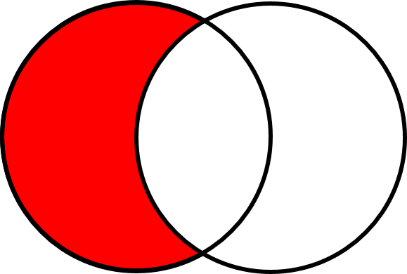
The `intersect()` function keeps the rows that appear in both of the datasets under consideration.  

There are many situations where we need to identify the rows in common between two (or more) datasets.  A very common example is where you have two datasets containing names (e.g. states, elements, species) and you want to find the names that are in both datasets.  An intersect operation allows you to do this.  

Let's consider another example.  You would like to perform analysis examining how water quality in a stream affects the health of fish.  The USGS has collected water quality samples periodically on this stream.  The EPA has collected fish tissue samples on this same stream, though their efforts were not coordinated so they didn't always sample on the same day.  You would like to only analyze data for which there were both fish and water samples collected on the same day.  

<br/>

Let's load in tables of sampling dates from each of the agencies  (EPA and USGS).  
```{r message=FALSE, warning=FALSE}
dates_EPA <- read_csv("https://stahlm.github.io/ENS_215/Data/Sampling_dates_EPA_fish_tissue.csv")
dates_USGS <- read_csv("https://stahlm.github.io/ENS_215/Data/Sampling_dates_USGS_water_quality.csv")
```

Take a look at each of the data frames.  You'll see that they each have a `Year`, `Month`, and `Day` column.  

To determine which dates they have in common we can use `intersect`
```{r}
dates_common <- intersect(dates_EPA, dates_USGS)
```
+ How many dates do we have both fish tissue and water quality sampling events?  


<br/>


#### Find set differences with `setdiff`
![](http://stahlm.github.io/ENS_215/Lectures/Images/set_diff.png){width=250}

<br/>

The difference between sets can be obtained by using the `setdiff()` function.  The `setdiff()` function returns the rows that appear in set A but not in set B, where `A` is the first set specified in `setdiff()` and `B` is the 2^nd^ set specified.  

Let's continue using our USGS and EPA sampling dates to test out the `setdiff()` function.  First let's determine the dates where there are only USGS (water quality) samples

```{r}
dates_only_USGS <- setdiff(dates_USGS, dates_EPA)
```

+ How many days are there where only the USGS samples are available?  

<br/>

Now you should determine the days when there are only EPA (fish tissue) samples 
```{r}
# Your code here
```
+ How many days are there where only the EPA samples are available?  


```{r echo=FALSE, eval=FALSE}

dates_EPA_only <- setdiff(dates_EPA, dates_USGS)

```

<br/>

#### Find the `union` of sets
![](http://stahlm.github.io/ENS_215/Lectures/Images/set_union.png){width=250} 

<br/>

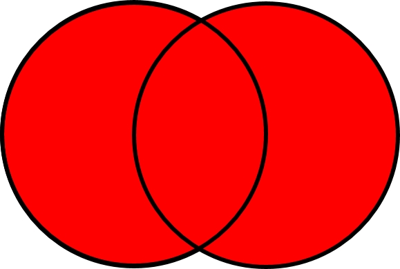
The union of sets finds the rows that appear in set A or set B (as illustrated in the venn-diagram above).  Duplicates are removed -- thus any row that appears in both A and B will only appear ONCE in the union.  

Let's take the union of the USGS and EPA sampling dates.  This will tell us how many unique dates samples were collected on.  

```{r}
dates_USGS_EPA <- union(dates_USGS, dates_EPA)
```

+ How many rows are there in the `dates_USGS_EPA` data frame?
+ Why is the number of rows less than the sum of the number of rows in `dates_USGS` and `dates_EPA`?

<br/>


### Combine columns (variables) with `bind_cols`
Bind columns is a very straightforward function.  It simply pastes two data frames side-by-side, thus making a single, larger data frame.  While `bind_cols()` is useful, you should be careful when using it as it does not do anything to ensure that observations (rows) are properly matched - thus it is up to you to make sure that the ordering of the rows makes sense before binding two data frames with `bind_cols()`  

Let's try out a quick example.  

First let's create two new data frames 
```{r}
years_USGS <- select(dates_USGS, Year) 
months_days_USGS <- select(dates_USGS, Month, Day) 
```

<br/>

Take a look at both of these data frames.  Once it makes sense to you, then let's use `bind_cols()` to join the data.  While this is a bit of an artificial example, it nonetheless highlights how you can use `bind_cols()`.

```{r}
bind_example <- bind_cols(years_USGS, months_days_USGS)

head(bind_example)
```


<br/>

### Combine datasets with `joins`

Joins allow you to combine the columns of two dataset, matching the rows by a **key**.  The **key** is a column (variable) or set of columns that contains identifying information for each row (observation).  For example if the key might be a column with a location name (e.g. US state) if we wanted to join two datasets with data for each US state.  The key also be a set of columns - for example we might want to join two dataset and match the rows by "Year", "Month", and "Day", which are contained in three columns in each dataset.  

These concepts will make much more sense as you work through the examples in the following sections.  


See [Chapter 3.7 of ModernDive](https://moderndive.com/v2/wrangling.html#joins) for a nice discussion of joins.  You can also see [Chapter 19 of R4DS](https://r4ds.hadley.nz/joins) for additional details on joining data frames.   

The diagrams below help to graphically illustrate how columns from two datasets are joined - matching up the rows according to the **key** variable.  

![_Image source: R4DS_](https://stahlm.github.io/ENS_215/Lectures/Images/join-setup.png)

<br/>
<br/>

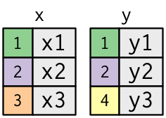
The **key** variable(s) (the numbers in the colored cells) are matched between the two datasets to be joined and then the columns are merged with the matching rows retained and aligned.  

![_Image source: R4DS_](https://stahlm.github.io/ENS_215/Lectures/Images/join-inner.png)

<br/>

There are two types of joins - inner joins and outer joins.  

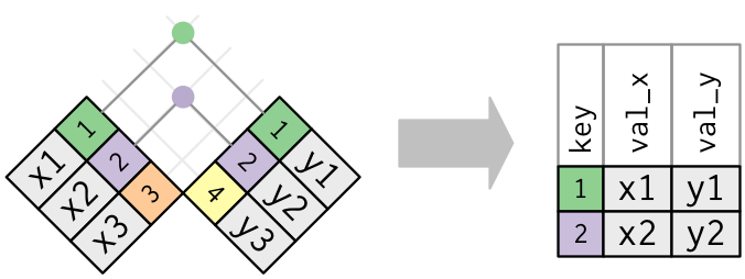
An **inner join** will match observations when their keys are equal and the output data frame contains columns from both datasets for only the observations common to both datasets.  Thus unmatched rows are not included in the output of an **inner join**  

An **outer join** differs in that it keeps observations that appear in at least one of the tables.  There are three types of outer joins:  

+ **Left join** keeps all observations (rows) in dataset `x`
+ **Right join** keeps all observations (rows) in dataset `y`
+ **Full join** keeps all observations (rows) in dataset `x` and `y`

Where `x` and `y` are the 1^st^ and 2^nd^ datasets respectively specified in the join function.  

<br/>

Let's load in NOAA temperature data that we would like to join with our NOAA precipitation data.  The NOAA temperature dataset has monthly temperature data for all the state in the US for every year from 1895 through 2017.  

```{r warning=FALSE, message=FALSE}
temperature_data <- read_csv("https://stahlm.github.io/ENS_215/Data/NOAA_State_Temp_Lab_Data.csv")
```


Let's remove the year 2016 data for New York from the temperature dataset.  We are doing this, since it will help to illustrate how unmatched observations are dealt with during joins.  

```{r}
temperature_data <- filter(temperature_data, !(Year == 2016 & state_cd == "NY")) # remove data for NY in year 2016
```


<br/>

#### Joins: `inner_join`

![_Image source: R4DS_](https://stahlm.github.io/ENS_215/Lectures/Images/join-inner.png)

<br/>

An `inner_join` (shown in the diagram above) is the simplest type of join.  Let's join our precipitation and temperature data so that we can can precip and temp data for each observation.  


First let's take a look at the first few rows of each dataset.  I've highlighted the **key** variables (columns) in yellow. 
```{r eval = FALSE}
head(precip_combined)
head(temperature_data)
```

```{r echo=FALSE, message=FALSE, warning=FALSE}
library(kableExtra)
head(precip_combined) %>% 
  kable() %>% 
  kable_styling(bootstrap_options = "condensed", position = "center") %>% 
  column_spec(column = c(1,2,4), background = "yellow") %>% 
  column_spec(column = c(3), background = "lightgrey") 

head(temperature_data) %>% 
  kable() %>% 
  kable_styling(bootstrap_options = "condensed", position = "center") %>% 
  column_spec(column = c(1,2,4), background = "yellow") %>% 
  column_spec(column = c(3), background = "lightgrey") 


```

<br/>

Now let's join the temperature and precipitation data using an `inner_join()`
```{r}
climate_data <- inner_join(precip_combined, temperature_data)
```

In the message above you see that `inner_join()`, joined the datasets by the "Year", "Month", "state_cd" columns (i.e. it used the values in these columns to match rows (_observations_) ).  You are able to explicitly specify the columns you would like to join by, simply by passing `by = c("Column name 1", "Column name 2",...)` as an argument in the `inner_join` function (or any of the other join functions).  However, the join functions in `tidyr` are smart and will join by all of the common columns (variables) unless you specify otherwise.  

<br/>

The first few rows of the joined table looks like this
```{r echo = FALSE}
head(climate_data)  %>% 
  kable() %>% 
  kable_styling(bootstrap_options = "condensed", position = "center")
```

<br/>

Ok now, take a closer look at the joined dataset `climate_data` and make sure you understand what is going on.  

+ What years does `climate_data` have observations for Massachusetts? Does this make sense to you?
+ What years does `climate_data` have observations for New York?  Does this make sense to you?

<br/>

#### Joins: `left_join`

![_Image source: R4DS_](https://stahlm.github.io/ENS_215/Lectures/Images/join-left.png)

<br/>

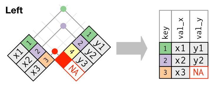
Now let's perform a `left_join` to add variables (columns) from `temperature_data` to `precip_combined`.  The `left_join` will only add observations from `temperature_data` that match observations in `precip_combined`.  In this case, the observations are matched according to the `Year`, `Month`, and `state_cd` in each table.  

```{r}
climate_data <- left_join(precip_combined, temperature_data)
```

+ Do any of the columns have missing data (i.e. `NA`s)?  Does this make sense?  


The `left_join` is the most commonly used **outer join** operation and should be your default outer join choice unless you have a compelling reason to use another join.  However, there are other joins available and we'll introduce these below so that you are aware of them.  


<br/>

##### Exercise 
Let's use `left_join` to join a dataset containing information about the region the states are in to the our dataset `climate_data`.  

First you should load in the dataset with the region data.  
```{r message=FALSE}
regions_data <- read_csv("https://stahlm.github.io/ENS_215/Data/state_regions.csv")
```

Take a look at the data to make sure everything looks ok.  

Now, you should join this data to your `climate_data` so that you have regions associated with each observation in the `climate_data`.  Note you may have to make some slight modifications to one of the datasets prior to joining them.  

```{r echo=FALSE, message=FALSE}
regions_data <- mutate(regions_data, state_cd = State_abb)
a <- left_join(climate_data, regions_data)
```

Once you've joined the data take a look and make sure you understand exactly what happened.  

<br/>


#### Joins: `right_join`
 
![_Image source: R4DS_](https://stahlm.github.io/ENS_215/Lectures/Images/join-right.png)

<br/>

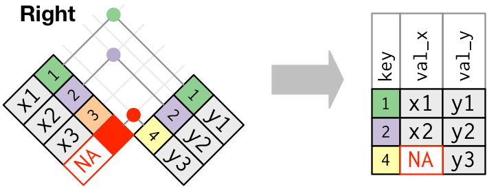
The `right_join` is conceptually similar to `left_join` except it matches in the opposite direction as `left_join`.  

Test out `right_join` on your `precip_combined` and `temperature_data`.  Examine the joined dataset and make sure you understand what happened.  Try the join twice (switching the order of the datasets in the function calls) and make sure it is clear what is happening?  

Is one of your `right_joins` equivalent to your `left_join` performed earlier on these datasets?

```{r}
# Your code here
```


```{r eval=FALSE, echo=FALSE, message=FALSE}
right_join(precip_combined, temperature_data)
right_join(temperature_data, precip_combined)
```

 
<br/>


#### Joins: `full_join`

![_Image source: R4DS_](https://stahlm.github.io/ENS_215/Lectures/Images/join-full.png)

<br/>

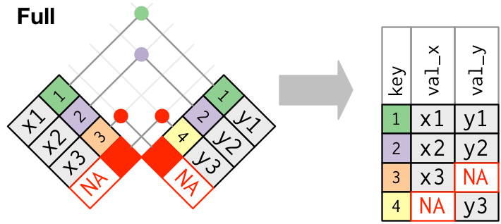
The `full_join` function joins the two datasets, keeping all values and all rows.  

Test out `full_join` on your `precip_combined` and `temperature_data`.  Examine the joined dataset and make sure you understand what happened.

```{r}
# Your code here 
```


```{r eval=FALSE, echo=FALSE, message=FALSE}

full_join(precip_combined, temperature_data)
full_join(temperature_data, precip_combined)

```

+ Does the order of the datasets in the `full_join()` function call make a difference in terms of the content of your joined dataset?  

<br/>



#### Exercise 

1. Load in the `gapminder` data and the dams data from lab 3.  Then add the population and per capita GDP to the dams data (using the 2007 gapminder data).  

Once you've joined these dataset, try some additional exploratory analysis of the enhanced dams data that now has population and per capita GDP data. 

The dams data and gapminder data are here
```{r eval = FALSE}
library(gapminder) 

my_gap <- gapminder
dams_data <- read_csv("https://stahlm.github.io/ENS_215/Data/Dams_FAO_SelectCols_LabData.csv")
```

```{r eval=FALSE, echo=FALSE, message=FALSE, warning=FALSE}
dams_data <- rename(dams_data, country = Country)

my_gap <- filter(my_gap, year == 2007) %>% 
  select(-lifeExp, -continent, -year)

dams_enhanced <- left_join(dams_data, my_gap)
```

<br/>

2. Practice additional joins and merges with the datasets in this lesson or with datasets in other lessons or labs.  

***