{
"cells": [
{
"cell_type": "markdown",
"metadata": {},
"source": [
"# Chapter2\n",
"D3.js in Actionの2章の勉強ノートです。\n"
]
},
{
"cell_type": "code",
"execution_count": 1,
"metadata": {
"collapsed": false
},
"outputs": [
{
"name": "stdout",
"output_type": "stream",
"text": [
"loaded nvd3 IPython extension\n",
"run nvd3.ipynb.initialize_javascript() to set up the notebook\n",
"help(nvd3.ipynb.initialize_javascript) for options\n"
]
},
{
"data": {
"text/html": [
""
],
"text/plain": [
""
]
},
"metadata": {},
"output_type": "display_data"
},
{
"data": {
"application/javascript": [
"$.getScript(\"https://cdnjs.cloudflare.com/ajax/libs/nvd3/1.7.0/nv.d3.min.js\")"
],
"text/plain": [
""
]
},
"metadata": {},
"output_type": "display_data"
},
{
"data": {
"application/javascript": [
"$.getScript(\"https://cdnjs.cloudflare.com/ajax/libs/d3/3.5.5/d3.min.js\", function() {\n",
" $.getScript(\"https://cdnjs.cloudflare.com/ajax/libs/nvd3/1.7.0/nv.d3.min.js\", function() {})});"
],
"text/plain": [
""
]
},
"metadata": {},
"output_type": "display_data"
},
{
"data": {
"text/html": [
""
],
"text/plain": [
""
]
},
"metadata": {},
"output_type": "display_data"
},
{
"data": {
"text/html": [
""
],
"text/plain": [
""
]
},
"metadata": {},
"output_type": "display_data"
}
],
"source": [
"%load_ext sage\n",
"from IPython.core.display import HTML\n",
"from string import Template\n",
"import json\n",
"import nvd3\n",
"nvd3.ipynb.initialize_javascript(use_remote=True)"
]
},
{
"cell_type": "markdown",
"metadata": {},
"source": [
"## データの読み込み\n",
"D3では様々なデータをサポートしています。\n",
"- TEXT: d3.text()\n",
"- XML: d3.xml()\n",
"- CSV: d3.csv()\n",
"- JSON: d3.json()\n",
"- HTML: d3.html()\n",
"\n",
"pythonとのインタフェースを取ることを考えると、一般的に構造を保持できるJSONとCSVがデータの受け渡しに使われるます。\n",
"\n",
"例として以下のようなcities.csvを読み込んでみましょう。"
]
},
{
"cell_type": "code",
"execution_count": 2,
"metadata": {
"collapsed": false
},
"outputs": [
{
"name": "stdout",
"output_type": "stream",
"text": [
"\"label\",\"population\",\"country\",\"x\",\"y\"\r\n",
"\"San Francisco\", 750000,\"USA\",37,-122\r\n",
"\"Fresno\", 500000,\"USA\",36,-119\r\n",
"\"Lahore\",12500000,\"Pakistan\",31,74\r\n",
"\"Karachi\",13000000,\"Pakistan\",24,67\r\n",
"\"Rome\",2500000,\"Italy\",41,12\r\n",
"\"Naples\",1000000,\"Italy\",40,14\r\n",
"\"Rio\",12300000,\"Brazil\",-22,-43\r\n",
"\"Sao Paolo\",12300000,\"Brazil\",-23,-46"
]
}
],
"source": [
"!cat data/cities.csv"
]
},
{
"cell_type": "markdown",
"metadata": {},
"source": [
"読み込まれたデータは、function(error, data)形式のコールバックで与えられます。\n",
"このコールバックの中で実行したい処理を記述する方式になります。"
]
},
{
"cell_type": "code",
"execution_count": 3,
"metadata": {
"collapsed": false
},
"outputs": [
{
"data": {
"application/javascript": [
"d3.csv(\"data/cities.csv\",function(error,data) {console.log(error,data)});"
],
"text/plain": [
""
]
},
"metadata": {},
"output_type": "display_data"
}
],
"source": [
"%%javascript\n",
"d3.csv(\"data/cities.csv\",function(error,data) {console.log(error,data)});"
]
},
{
"cell_type": "markdown",
"metadata": {
"collapsed": true
},
"source": [
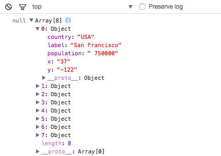
"javascriptのコンソールに以下のようにデータの内容が出力されます。\n",
"\n",
"\n"
]
},
{
"cell_type": "markdown",
"metadata": {},
"source": [
"これを見るとCSVのデータがヘッダのカラム名をキーとする辞書の配列として渡されていることがわかります。"
]
},
{
"cell_type": "markdown",
"metadata": {},
"source": [
"## Pythonデータの受け渡し\n",
"jupyterの計算結果をD3に渡す方法を以下に紹介します。\n",
"\n",
"jsonとTemplateライブラリを使用します。"
]
},
{
"cell_type": "code",
"execution_count": 5,
"metadata": {
"collapsed": true
},
"outputs": [],
"source": [
"from string import Template\n",
"import json\n",
"import pandas as pd"
]
},
{
"cell_type": "markdown",
"metadata": {},
"source": [
"pandasを使ってcities.csvを読み込み、データフレームdfにセットします。"
]
},
{
"cell_type": "code",
"execution_count": 6,
"metadata": {
"collapsed": false
},
"outputs": [
{
"data": {
"text/html": [
"\n",
"
\n",
" \n",
" \n",
" | \n",
" label | \n",
" population | \n",
" country | \n",
" x | \n",
" y | \n",
"
\n",
" \n",
" \n",
" \n",
" | 0 | \n",
" San Francisco | \n",
" 750000 | \n",
" USA | \n",
" 37 | \n",
" -122 | \n",
"
\n",
" \n",
" | 1 | \n",
" Fresno | \n",
" 500000 | \n",
" USA | \n",
" 36 | \n",
" -119 | \n",
"
\n",
" \n",
" | 2 | \n",
" Lahore | \n",
" 12500000 | \n",
" Pakistan | \n",
" 31 | \n",
" 74 | \n",
"
\n",
" \n",
" | 3 | \n",
" Karachi | \n",
" 13000000 | \n",
" Pakistan | \n",
" 24 | \n",
" 67 | \n",
"
\n",
" \n",
" | 4 | \n",
" Rome | \n",
" 2500000 | \n",
" Italy | \n",
" 41 | \n",
" 12 | \n",
"
\n",
" \n",
"
\n",
"
\n",
"
a
\n",
"
b
\n",
"
c
\n",
"
d
\n",
"
\n",
"
a
\n",
"
b
\n",
"
c
\n",
"
d
\n",
"
\n",
" \n",
"
"
],
"text/plain": [
""
]
},
"metadata": {},
"output_type": "display_data"
}
],
"source": [
"%%HTML\n",
"\n",
" \n",
"
"
]
},
{
"cell_type": "code",
"execution_count": 20,
"metadata": {
"collapsed": false
},
"outputs": [
{
"data": {
"application/javascript": [
"d3.select('#ex4').select(\"svg\")\n",
" .selectAll(\"rect\")\n",
" .data([15, 50, 22, 8, 100, 10])\n",
" .enter()\n",
" .append(\"rect\")\n",
" .attr(\"width\", 10)\n",
" .attr(\"height\", function(d) {return d;})\n",
" .style(\"fill\", \"blue\")\n",
" .style(\"stroke\", \"red\")\n",
" .style(\"stroke-width\", \"1px\")\n",
" .style(\"opacity\", .25)\n",
" .attr(\"x\", function(d, i) {return i * 10})\n",
" .attr(\"y\", function(d) {return 100 - d;});"
],
"text/plain": [
""
]
},
"metadata": {},
"output_type": "display_data"
}
],
"source": [
"%%javascript\n",
"d3.select('#ex4').select(\"svg\")\n",
" .selectAll(\"rect\")\n",
" .data([15, 50, 22, 8, 100, 10])\n",
" .enter()\n",
" .append(\"rect\")\n",
" .attr(\"width\", 10)\n",
" .attr(\"height\", function(d) {return d;})\n",
" .style(\"fill\", \"blue\")\n",
" .style(\"stroke\", \"red\")\n",
" .style(\"stroke-width\", \"1px\")\n",
" .style(\"opacity\", .25)\n",
" .attr(\"x\", function(d, i) {return i * 10})\n",
" .attr(\"y\", function(d) {return 100 - d;});"
]
},
{
"cell_type": "markdown",
"metadata": {
"collapsed": true
},
"source": [
"## CSVデータから棒グラフを作る\n",
"2章のメインテーマは、CSVファイルから棒グラフを作成することです。\n",
"\n",
"例題にしたがって、cities.csvから棒グラフを作ってみます。"
]
},
{
"cell_type": "code",
"execution_count": 21,
"metadata": {
"collapsed": false
},
"outputs": [
{
"data": {
"text/html": [
"\n",
" \n",
"
"
],
"text/plain": [
""
]
},
"metadata": {},
"output_type": "display_data"
}
],
"source": [
"%%HTML\n",
"\n",
" \n",
"
"
]
},
{
"cell_type": "code",
"execution_count": 22,
"metadata": {
"collapsed": false
},
"outputs": [
{
"data": {
"application/javascript": [
"// dataフォルダのcities.csvを読み込み、dataViz関数を呼び出す\n",
"d3.csv(\"data/cities.csv\",function(error,data) {dataViz(data);});\n",
"function dataViz(incomingData) {\n",
" var maxPopulation = d3.max(incomingData, function(el) {\n",
" // 人口のデータを文字列から数値に変換\n",
" return parseInt(el.population);}\n",
" );\n",
" // 人口の最大値を0-230の範囲にスケーリングするyScaleを作成\n",
" var yScale = d3.scale.linear().domain([0,maxPopulation]).range([0,230]);\n",
" // 棒グラフの作成\n",
" d3.select('#ex5').select(\"svg\").attr(\"style\",\"height: 240px; width: 300px;\");\n",
" d3.select(\"#ex5 svg\")\n",
" .selectAll(\"rect\")\n",
" .data(incomingData)\n",
" .enter()\n",
" .append(\"rect\")\n",
" .attr(\"width\", 25)\n",
" .attr(\"height\", function(d) {return yScale(parseInt(d.population));})\n",
" .attr(\"x\", function(d,i) {return i * 30;})\n",
" .attr(\"y\", function(d) {return 240 - yScale(parseInt(d.population));})\n",
" .style(\"fill\", \"blue\")\n",
" .style(\"stroke\", \"red\")\n",
" .style(\"stroke-width\", \"1px\")\n",
" .style(\"opacity\", .25);\n",
"}"
],
"text/plain": [
""
]
},
"metadata": {},
"output_type": "display_data"
}
],
"source": [
"%%javascript\n",
"// dataフォルダのcities.csvを読み込み、dataViz関数を呼び出す\n",
"d3.csv(\"data/cities.csv\",function(error,data) {dataViz(data);});\n",
"function dataViz(incomingData) {\n",
" var maxPopulation = d3.max(incomingData, function(el) {\n",
" // 人口のデータを文字列から数値に変換\n",
" return parseInt(el.population);}\n",
" );\n",
" // 人口の最大値を0-230の範囲にスケーリングするyScaleを作成\n",
" var yScale = d3.scale.linear().domain([0,maxPopulation]).range([0,230]);\n",
" // 棒グラフの作成\n",
" d3.select('#ex5').select(\"svg\").attr(\"style\",\"height: 240px; width: 300px;\");\n",
" d3.select(\"#ex5 svg\")\n",
" .selectAll(\"rect\")\n",
" .data(incomingData)\n",
" .enter()\n",
" .append(\"rect\")\n",
" .attr(\"width\", 25)\n",
" .attr(\"height\", function(d) {return yScale(parseInt(d.population));})\n",
" .attr(\"x\", function(d,i) {return i * 30;})\n",
" .attr(\"y\", function(d) {return 240 - yScale(parseInt(d.population));})\n",
" .style(\"fill\", \"blue\")\n",
" .style(\"stroke\", \"red\")\n",
" .style(\"stroke-width\", \"1px\")\n",
" .style(\"opacity\", .25);\n",
"}"
]
},
{
"cell_type": "code",
"execution_count": null,
"metadata": {
"collapsed": true
},
"outputs": [],
"source": []
}
],
"metadata": {
"kernelspec": {
"display_name": "Python 2",
"language": "python",
"name": "python2"
},
"language_info": {
"codemirror_mode": {
"name": "ipython",
"version": 2
},
"file_extension": ".py",
"mimetype": "text/x-python",
"name": "python",
"nbconvert_exporter": "python",
"pygments_lexer": "ipython2",
"version": "2.7.10"
}
},
"nbformat": 4,
"nbformat_minor": 0
}