{
"cells": [
{
"cell_type": "markdown",
"metadata": {
"slideshow": {
"slide_type": "slide"
}
},
"source": [
"#  CS 236756 - Technion - Intro to Machine Learning\n",
"---\n",
"#### Tal Daniel\n",
"\n",
"## Tutorial 03 - Linear Algebra & SVD\n",
"---\n"
]
},
{
"cell_type": "markdown",
"metadata": {
"slideshow": {
"slide_type": "subslide"
}
},
"source": [
"###
CS 236756 - Technion - Intro to Machine Learning\n",
"---\n",
"#### Tal Daniel\n",
"\n",
"## Tutorial 03 - Linear Algebra & SVD\n",
"---\n"
]
},
{
"cell_type": "markdown",
"metadata": {
"slideshow": {
"slide_type": "subslide"
}
},
"source": [
"###  Agenda\n",
"---\n",
"* [Linear Algebra Refresher](#-Linear-Algebra-Refresher)\n",
"* [Eigen Values and Vectors Decomposition](#-Eigenvalues-and-Eigenvectors)\n",
"* [Singular Value Decomposition (SVD)](#-Singular-Value-Decomposition-(SVD))\n",
"* [Recommended Videos](#-Recommended-Videos)\n",
"* [Credits](#-Credits)"
]
},
{
"cell_type": "markdown",
"metadata": {
"slideshow": {
"slide_type": "subslide"
}
},
"source": [
"####
Agenda\n",
"---\n",
"* [Linear Algebra Refresher](#-Linear-Algebra-Refresher)\n",
"* [Eigen Values and Vectors Decomposition](#-Eigenvalues-and-Eigenvectors)\n",
"* [Singular Value Decomposition (SVD)](#-Singular-Value-Decomposition-(SVD))\n",
"* [Recommended Videos](#-Recommended-Videos)\n",
"* [Credits](#-Credits)"
]
},
{
"cell_type": "markdown",
"metadata": {
"slideshow": {
"slide_type": "subslide"
}
},
"source": [
"####  Useful Resource\n",
"---\n",
"\n",
" The Matrix Cookbook\n",
""
]
},
{
"cell_type": "code",
"execution_count": 1,
"metadata": {
"slideshow": {
"slide_type": "skip"
}
},
"outputs": [],
"source": [
"# imports for the tutorial\n",
"import numpy as np\n",
"import pandas as pd\n",
"import matplotlib.pyplot as plt\n",
"%matplotlib notebook"
]
},
{
"cell_type": "markdown",
"metadata": {
"slideshow": {
"slide_type": "slide"
}
},
"source": [
"##
Useful Resource\n",
"---\n",
"\n",
" The Matrix Cookbook\n",
""
]
},
{
"cell_type": "code",
"execution_count": 1,
"metadata": {
"slideshow": {
"slide_type": "skip"
}
},
"outputs": [],
"source": [
"# imports for the tutorial\n",
"import numpy as np\n",
"import pandas as pd\n",
"import matplotlib.pyplot as plt\n",
"%matplotlib notebook"
]
},
{
"cell_type": "markdown",
"metadata": {
"slideshow": {
"slide_type": "slide"
}
},
"source": [
"##  Linear Algebra Refresher\n",
"---\n",
"###
Linear Algebra Refresher\n",
"---\n",
"###  Vectors\n",
"---\n",
"* Geometric object that has both a magnitude and direction\n",
" * $ x = \\begin{bmatrix} x_{1} \\\\ x_{2} \\\\ \\vdots \\\\ x_{n} \\end{bmatrix} = (x_1, x_2, ..., x_n)^{T} \\in \\mathcal{R}^n$\n",
"* Magnitude of a vector: $||x|| = \\sqrt{x^{T}x} = \\sqrt{x_1^2 +x_2^2 +... +x_n^2}$\n",
"* **Cardinality** of a vector - the number of non zero elements"
]
},
{
"cell_type": "code",
"execution_count": 2,
"metadata": {
"slideshow": {
"slide_type": "subslide"
}
},
"outputs": [
{
"name": "stdout",
"output_type": "stream",
"text": [
"v:\n",
"[[ 16]\n",
" [ 0]\n",
" [ 19]\n",
" [-16]\n",
" [ -9]\n",
" [ 10]]\n",
"v^T:\n",
"[[ 16 0 19 -16 -9 10]]\n"
]
}
],
"source": [
"# let's see some vectors\n",
"v = np.random.randint(low=-20, high=20, size=(6, 1))\n",
"print(\"v:\")\n",
"print(v)\n",
"print(\"v^T:\")\n",
"print(v.T)"
]
},
{
"cell_type": "code",
"execution_count": 3,
"metadata": {
"slideshow": {
"slide_type": "subslide"
}
},
"outputs": [
{
"name": "stdout",
"output_type": "stream",
"text": [
"magnitude of v:\n",
"32.46536616149585\n",
"cardinality- non zero elements:\n",
"5\n"
]
}
],
"source": [
"print(\"magnitude of v:\")\n",
"print(np.sqrt(np.sum(np.square(v))))\n",
"print(\"cardinality- non zero elements:\")\n",
"print(np.sum(v != 0))"
]
},
{
"cell_type": "markdown",
"metadata": {
"slideshow": {
"slide_type": "slide"
}
},
"source": [
"###
Vectors\n",
"---\n",
"* Geometric object that has both a magnitude and direction\n",
" * $ x = \\begin{bmatrix} x_{1} \\\\ x_{2} \\\\ \\vdots \\\\ x_{n} \\end{bmatrix} = (x_1, x_2, ..., x_n)^{T} \\in \\mathcal{R}^n$\n",
"* Magnitude of a vector: $||x|| = \\sqrt{x^{T}x} = \\sqrt{x_1^2 +x_2^2 +... +x_n^2}$\n",
"* **Cardinality** of a vector - the number of non zero elements"
]
},
{
"cell_type": "code",
"execution_count": 2,
"metadata": {
"slideshow": {
"slide_type": "subslide"
}
},
"outputs": [
{
"name": "stdout",
"output_type": "stream",
"text": [
"v:\n",
"[[ 16]\n",
" [ 0]\n",
" [ 19]\n",
" [-16]\n",
" [ -9]\n",
" [ 10]]\n",
"v^T:\n",
"[[ 16 0 19 -16 -9 10]]\n"
]
}
],
"source": [
"# let's see some vectors\n",
"v = np.random.randint(low=-20, high=20, size=(6, 1))\n",
"print(\"v:\")\n",
"print(v)\n",
"print(\"v^T:\")\n",
"print(v.T)"
]
},
{
"cell_type": "code",
"execution_count": 3,
"metadata": {
"slideshow": {
"slide_type": "subslide"
}
},
"outputs": [
{
"name": "stdout",
"output_type": "stream",
"text": [
"magnitude of v:\n",
"32.46536616149585\n",
"cardinality- non zero elements:\n",
"5\n"
]
}
],
"source": [
"print(\"magnitude of v:\")\n",
"print(np.sqrt(np.sum(np.square(v))))\n",
"print(\"cardinality- non zero elements:\")\n",
"print(np.sum(v != 0))"
]
},
{
"cell_type": "markdown",
"metadata": {
"slideshow": {
"slide_type": "slide"
}
},
"source": [
"###  Inner Product Space\n",
"---\n",
"* A mapping $\\langle \\cdot, \\cdot \\rangle : V \\times V \\rightarrow F$ that satisfies:\n",
" * Conjucate Symmetry: $\\langle x, y \\rangle = \\overline{\\langle y, x \\rangle} $\n",
" * Linearity in the First Argument: \n",
" * $\\langle a \\cdot x, y \\rangle = a \\cdot \\langle x, y \\rangle$\n",
" * $\\langle x + z, y \\rangle = \\langle x, y \\rangle + \\langle z, y \\rangle$\n",
" * Positive-definiteness: \n",
" * $\\langle x, x \\rangle \\geq 0$\n",
" * $\\langle x, x \\rangle = 0 \\rightarrow x=0$"
]
},
{
"cell_type": "markdown",
"metadata": {
"slideshow": {
"slide_type": "subslide"
}
},
"source": [
"\n",
"* Common Inner Products:\n",
" * Real Vector: $\\langle x, y \\rangle = x^{T} y$\n",
" * Real Matrix: $\\langle A, B \\rangle = \\textit{trace}(AB^{T})$\n",
" * Random Variables: $\\langle x, y \\rangle = \\mathbb{E}[x \\cdot y]$\n"
]
},
{
"cell_type": "markdown",
"metadata": {
"slideshow": {
"slide_type": "subslide"
}
},
"source": [
"* Properties of **Dot Product**:\n",
" * Distributiveness: \n",
" * $(a + b)\\cdot c = a \\cdot c + b \\cdot c$\n",
" * $a \\cdot (b+c) = a\\cdot b + a\\cdot c$\n",
" * Linearity: $(\\lambda a)\\cdot b= a \\cdot (\\lambda b) = \\lambda(a \\cdot b)$\n",
" * Symmetry: $a \\cdot b= b\\cdot a$\n",
" * Non-Negativity: $\\forall a \\neq 0, a\\cdot a >0 , a \\cdot a =0 \\iff a=0$"
]
},
{
"cell_type": "code",
"execution_count": 4,
"metadata": {
"slideshow": {
"slide_type": "subslide"
}
},
"outputs": [
{
"name": "stdout",
"output_type": "stream",
"text": [
"a:\n",
"[[1.]\n",
" [1.]\n",
" [1.]\n",
" [1.]\n",
" [1.]]\n",
"b:\n",
"[[ 3]\n",
" [-4]\n",
" [ 5]\n",
" [ 8]\n",
" [-4]]\n",
"a.T.dot(b)=\n",
"[[8.]]\n",
"the same as a.T @ b:\n",
"[[8.]]\n"
]
}
],
"source": [
"# let's see some dot products\n",
"a = np.ones((5,1))\n",
"b = np.random.randint(low=-10, high=10, size=(5,1))\n",
"print(\"a:\")\n",
"print(a)\n",
"print(\"b:\")\n",
"print(b)\n",
"print(\"a.T.dot(b)=\")\n",
"print(a.T.dot(b))\n",
"print(\"the same as a.T @ b:\")\n",
"print(a.T @ b)"
]
},
{
"cell_type": "code",
"execution_count": 5,
"metadata": {
"slideshow": {
"slide_type": "subslide"
}
},
"outputs": [
{
"name": "stdout",
"output_type": "stream",
"text": [
"a + 0.5=\n",
"[[1.5]\n",
" [1.5]\n",
" [1.5]\n",
" [1.5]\n",
" [1.5]]\n",
"(a + 2 * a).T @ b\n",
"[[24.]]\n",
"the same as a.T @ b + (2 * a).T @ b\n",
"[[24.]]\n"
]
}
],
"source": [
"print(\"a + 0.5=\")\n",
"print(a + 0.5)\n",
"print(\"(a + 2 * a).T @ b\")\n",
"print((a + 2 * a).T @ b)\n",
"print(\"the same as a.T @ b + (2 * a).T @ b\")\n",
"print(a.T @ b + (2 * a).T @ b)"
]
},
{
"cell_type": "markdown",
"metadata": {
"slideshow": {
"slide_type": "slide"
}
},
"source": [
"###
Inner Product Space\n",
"---\n",
"* A mapping $\\langle \\cdot, \\cdot \\rangle : V \\times V \\rightarrow F$ that satisfies:\n",
" * Conjucate Symmetry: $\\langle x, y \\rangle = \\overline{\\langle y, x \\rangle} $\n",
" * Linearity in the First Argument: \n",
" * $\\langle a \\cdot x, y \\rangle = a \\cdot \\langle x, y \\rangle$\n",
" * $\\langle x + z, y \\rangle = \\langle x, y \\rangle + \\langle z, y \\rangle$\n",
" * Positive-definiteness: \n",
" * $\\langle x, x \\rangle \\geq 0$\n",
" * $\\langle x, x \\rangle = 0 \\rightarrow x=0$"
]
},
{
"cell_type": "markdown",
"metadata": {
"slideshow": {
"slide_type": "subslide"
}
},
"source": [
"\n",
"* Common Inner Products:\n",
" * Real Vector: $\\langle x, y \\rangle = x^{T} y$\n",
" * Real Matrix: $\\langle A, B \\rangle = \\textit{trace}(AB^{T})$\n",
" * Random Variables: $\\langle x, y \\rangle = \\mathbb{E}[x \\cdot y]$\n"
]
},
{
"cell_type": "markdown",
"metadata": {
"slideshow": {
"slide_type": "subslide"
}
},
"source": [
"* Properties of **Dot Product**:\n",
" * Distributiveness: \n",
" * $(a + b)\\cdot c = a \\cdot c + b \\cdot c$\n",
" * $a \\cdot (b+c) = a\\cdot b + a\\cdot c$\n",
" * Linearity: $(\\lambda a)\\cdot b= a \\cdot (\\lambda b) = \\lambda(a \\cdot b)$\n",
" * Symmetry: $a \\cdot b= b\\cdot a$\n",
" * Non-Negativity: $\\forall a \\neq 0, a\\cdot a >0 , a \\cdot a =0 \\iff a=0$"
]
},
{
"cell_type": "code",
"execution_count": 4,
"metadata": {
"slideshow": {
"slide_type": "subslide"
}
},
"outputs": [
{
"name": "stdout",
"output_type": "stream",
"text": [
"a:\n",
"[[1.]\n",
" [1.]\n",
" [1.]\n",
" [1.]\n",
" [1.]]\n",
"b:\n",
"[[ 3]\n",
" [-4]\n",
" [ 5]\n",
" [ 8]\n",
" [-4]]\n",
"a.T.dot(b)=\n",
"[[8.]]\n",
"the same as a.T @ b:\n",
"[[8.]]\n"
]
}
],
"source": [
"# let's see some dot products\n",
"a = np.ones((5,1))\n",
"b = np.random.randint(low=-10, high=10, size=(5,1))\n",
"print(\"a:\")\n",
"print(a)\n",
"print(\"b:\")\n",
"print(b)\n",
"print(\"a.T.dot(b)=\")\n",
"print(a.T.dot(b))\n",
"print(\"the same as a.T @ b:\")\n",
"print(a.T @ b)"
]
},
{
"cell_type": "code",
"execution_count": 5,
"metadata": {
"slideshow": {
"slide_type": "subslide"
}
},
"outputs": [
{
"name": "stdout",
"output_type": "stream",
"text": [
"a + 0.5=\n",
"[[1.5]\n",
" [1.5]\n",
" [1.5]\n",
" [1.5]\n",
" [1.5]]\n",
"(a + 2 * a).T @ b\n",
"[[24.]]\n",
"the same as a.T @ b + (2 * a).T @ b\n",
"[[24.]]\n"
]
}
],
"source": [
"print(\"a + 0.5=\")\n",
"print(a + 0.5)\n",
"print(\"(a + 2 * a).T @ b\")\n",
"print((a + 2 * a).T @ b)\n",
"print(\"the same as a.T @ b + (2 * a).T @ b\")\n",
"print(a.T @ b + (2 * a).T @ b)"
]
},
{
"cell_type": "markdown",
"metadata": {
"slideshow": {
"slide_type": "slide"
}
},
"source": [
"###  Outer Product\n",
"---\n",
"* Let:\n",
" * $a = (a_1, a_2, ..., a_n)^{T}$\n",
" * $b = (b_1, b_2, ..., b_n)^{T}$\n",
"* The outer product $ab^{T}$: $$ ab^{T} = \\begin{bmatrix} a_{1} \\\\ a_{2} \\\\ \\vdots \\\\ a_{n} \\end{bmatrix} [b_1, b_2, ..., b_n] = \\begin{pmatrix} a_1 b_1 & a_1 b_2 & \\cdots & a_1 b_n \\\\ a_2 b_1 & a_2 b_2 & \\cdots & a_2 b_n \\\\ \\vdots & \\vdots & \\ddots & \\vdots \\\\ a_n b_1 & a_n b_2 & \\cdots & a_n b_n \\end{pmatrix} $$"
]
},
{
"cell_type": "code",
"execution_count": 6,
"metadata": {
"slideshow": {
"slide_type": "subslide"
}
},
"outputs": [
{
"name": "stdout",
"output_type": "stream",
"text": [
"a:\n",
"[[0.68496376]\n",
" [0.51514789]\n",
" [0.97263803]\n",
" [0.47948046]\n",
" [0.97063678]]\n",
"b:\n",
"[[0.16180323]\n",
" [0.64818973]\n",
" [0.00683339]\n",
" [0.5219497 ]\n",
" [0.02569252]]\n"
]
}
],
"source": [
"# outer product\n",
"a = np.random.random(size=(5,1))\n",
"print(\"a:\")\n",
"print(a)\n",
"b = np.random.random(size=(5,1))\n",
"print(\"b:\")\n",
"print(b)"
]
},
{
"cell_type": "code",
"execution_count": 7,
"metadata": {
"slideshow": {
"slide_type": "subslide"
}
},
"outputs": [
{
"name": "stdout",
"output_type": "stream",
"text": [
"outer product: a @ b.T = \n",
"[[0.11082935 0.44398648 0.00468062 0.35751663 0.01759844]\n",
" [0.08335259 0.33391357 0.00352021 0.26888128 0.01323545]\n",
" [0.15737597 0.63045398 0.00664641 0.50766812 0.02498952]\n",
" [0.07758149 0.31079431 0.00327648 0.25026468 0.01231906]\n",
" [0.15705217 0.62915679 0.00663274 0.50662357 0.0249381 ]]\n"
]
}
],
"source": [
"ab_t = a @ b.T\n",
"print(\"outer product: a @ b.T = \")\n",
"print(ab_t)"
]
},
{
"cell_type": "markdown",
"metadata": {
"slideshow": {
"slide_type": "slide"
}
},
"source": [
"###
Outer Product\n",
"---\n",
"* Let:\n",
" * $a = (a_1, a_2, ..., a_n)^{T}$\n",
" * $b = (b_1, b_2, ..., b_n)^{T}$\n",
"* The outer product $ab^{T}$: $$ ab^{T} = \\begin{bmatrix} a_{1} \\\\ a_{2} \\\\ \\vdots \\\\ a_{n} \\end{bmatrix} [b_1, b_2, ..., b_n] = \\begin{pmatrix} a_1 b_1 & a_1 b_2 & \\cdots & a_1 b_n \\\\ a_2 b_1 & a_2 b_2 & \\cdots & a_2 b_n \\\\ \\vdots & \\vdots & \\ddots & \\vdots \\\\ a_n b_1 & a_n b_2 & \\cdots & a_n b_n \\end{pmatrix} $$"
]
},
{
"cell_type": "code",
"execution_count": 6,
"metadata": {
"slideshow": {
"slide_type": "subslide"
}
},
"outputs": [
{
"name": "stdout",
"output_type": "stream",
"text": [
"a:\n",
"[[0.68496376]\n",
" [0.51514789]\n",
" [0.97263803]\n",
" [0.47948046]\n",
" [0.97063678]]\n",
"b:\n",
"[[0.16180323]\n",
" [0.64818973]\n",
" [0.00683339]\n",
" [0.5219497 ]\n",
" [0.02569252]]\n"
]
}
],
"source": [
"# outer product\n",
"a = np.random.random(size=(5,1))\n",
"print(\"a:\")\n",
"print(a)\n",
"b = np.random.random(size=(5,1))\n",
"print(\"b:\")\n",
"print(b)"
]
},
{
"cell_type": "code",
"execution_count": 7,
"metadata": {
"slideshow": {
"slide_type": "subslide"
}
},
"outputs": [
{
"name": "stdout",
"output_type": "stream",
"text": [
"outer product: a @ b.T = \n",
"[[0.11082935 0.44398648 0.00468062 0.35751663 0.01759844]\n",
" [0.08335259 0.33391357 0.00352021 0.26888128 0.01323545]\n",
" [0.15737597 0.63045398 0.00664641 0.50766812 0.02498952]\n",
" [0.07758149 0.31079431 0.00327648 0.25026468 0.01231906]\n",
" [0.15705217 0.62915679 0.00663274 0.50662357 0.0249381 ]]\n"
]
}
],
"source": [
"ab_t = a @ b.T\n",
"print(\"outer product: a @ b.T = \")\n",
"print(ab_t)"
]
},
{
"cell_type": "markdown",
"metadata": {
"slideshow": {
"slide_type": "slide"
}
},
"source": [
"###  Vector Norms\n",
"---\n",
"* A norm on a vector sapce $\\Omega$ is a function $f: \\Omega \\rightarrow \\mathcal{R}$ with the following properties:\n",
" * Positive Scalability: $f(ax) = |a|f(x)$\n",
" * Triangle Inequality: $f(x+y) \\leq f(x) + f(y)$\n",
" * If $f(x) = 0 \\rightarrow x = 0$\n",
"* $l_1$ norm: $||x||_1 = \\sum_{i=1}^n |x_i| $"
]
},
{
"cell_type": "markdown",
"metadata": {
"slideshow": {
"slide_type": "subslide"
}
},
"source": [
"\n",
"* $l_2$ norm: $||x||_2 = \\sqrt{\\sum_{i=1}^n |x_i|^2} $\n",
" * For **Vectors**: $||x||_2^2 = x^{T}x$\n",
" * $l_2$-distance: $||x -y||_2^2 = (x-y)^{T}(x-y)= ||x||_2^2 -2x^{T}y + ||y||_2^2$\n",
"* $l_p$ norm: $||x||_p = (\\sum_{i=1}^n |x_i|^p)^{\\frac{1}{p}} $\n",
"* $l_{\\infty}$ norm: $||x||_{\\infty} = \\max{(|x_1|, |x_2|, ..., |x_n|)} $"
]
},
{
"cell_type": "markdown",
"metadata": {
"slideshow": {
"slide_type": "subslide"
}
},
"source": [
"
Vector Norms\n",
"---\n",
"* A norm on a vector sapce $\\Omega$ is a function $f: \\Omega \\rightarrow \\mathcal{R}$ with the following properties:\n",
" * Positive Scalability: $f(ax) = |a|f(x)$\n",
" * Triangle Inequality: $f(x+y) \\leq f(x) + f(y)$\n",
" * If $f(x) = 0 \\rightarrow x = 0$\n",
"* $l_1$ norm: $||x||_1 = \\sum_{i=1}^n |x_i| $"
]
},
{
"cell_type": "markdown",
"metadata": {
"slideshow": {
"slide_type": "subslide"
}
},
"source": [
"\n",
"* $l_2$ norm: $||x||_2 = \\sqrt{\\sum_{i=1}^n |x_i|^2} $\n",
" * For **Vectors**: $||x||_2^2 = x^{T}x$\n",
" * $l_2$-distance: $||x -y||_2^2 = (x-y)^{T}(x-y)= ||x||_2^2 -2x^{T}y + ||y||_2^2$\n",
"* $l_p$ norm: $||x||_p = (\\sum_{i=1}^n |x_i|^p)^{\\frac{1}{p}} $\n",
"* $l_{\\infty}$ norm: $||x||_{\\infty} = \\max{(|x_1|, |x_2|, ..., |x_n|)} $"
]
},
{
"cell_type": "markdown",
"metadata": {
"slideshow": {
"slide_type": "subslide"
}
},
"source": [
" "
]
},
{
"cell_type": "code",
"execution_count": 8,
"metadata": {
"slideshow": {
"slide_type": "subslide"
}
},
"outputs": [
{
"name": "stdout",
"output_type": "stream",
"text": [
"a:\n",
"[[0.20110422]\n",
" [0.3103417 ]\n",
" [0.25755954]\n",
" [0.84291866]\n",
" [0.00855558]]\n",
"l-1 norm: \n",
"1.6204796988041368\n",
"l-2 norm: \n",
"0.9558644554276373\n",
"l-infinity norm:\n",
"0.8429186563888088\n"
]
}
],
"source": [
"# norms and distance\n",
"a = np.random.random(size=(5,1))\n",
"print(\"a:\")\n",
"print(a)\n",
"print(\"l-1 norm: \")\n",
"print(np.sum(abs(a)))\n",
"print(\"l-2 norm: \")\n",
"print(np.sqrt(np.sum(np.square(a))))\n",
"print(\"l-infinity norm:\")\n",
"print(np.max(abs(a)))"
]
},
{
"cell_type": "code",
"execution_count": 9,
"metadata": {
"slideshow": {
"slide_type": "subslide"
}
},
"outputs": [
{
"name": "stdout",
"output_type": "stream",
"text": [
"b:\n",
"[[0.59011591]\n",
" [0.77681828]\n",
" [0.31464032]\n",
" [0.78600795]\n",
" [0.85952156]]\n",
"l-2 distance between a and b:\n",
"[[1.04860414]]\n"
]
}
],
"source": [
"b = np.random.random(size=(5,1))\n",
"print(\"b:\")\n",
"print(b)\n",
"print(\"l-2 distance between a and b:\")\n",
"print(np.sqrt((a - b).T @ (a - b)))"
]
},
{
"cell_type": "markdown",
"metadata": {
"slideshow": {
"slide_type": "slide"
}
},
"source": [
"###
"
]
},
{
"cell_type": "code",
"execution_count": 8,
"metadata": {
"slideshow": {
"slide_type": "subslide"
}
},
"outputs": [
{
"name": "stdout",
"output_type": "stream",
"text": [
"a:\n",
"[[0.20110422]\n",
" [0.3103417 ]\n",
" [0.25755954]\n",
" [0.84291866]\n",
" [0.00855558]]\n",
"l-1 norm: \n",
"1.6204796988041368\n",
"l-2 norm: \n",
"0.9558644554276373\n",
"l-infinity norm:\n",
"0.8429186563888088\n"
]
}
],
"source": [
"# norms and distance\n",
"a = np.random.random(size=(5,1))\n",
"print(\"a:\")\n",
"print(a)\n",
"print(\"l-1 norm: \")\n",
"print(np.sum(abs(a)))\n",
"print(\"l-2 norm: \")\n",
"print(np.sqrt(np.sum(np.square(a))))\n",
"print(\"l-infinity norm:\")\n",
"print(np.max(abs(a)))"
]
},
{
"cell_type": "code",
"execution_count": 9,
"metadata": {
"slideshow": {
"slide_type": "subslide"
}
},
"outputs": [
{
"name": "stdout",
"output_type": "stream",
"text": [
"b:\n",
"[[0.59011591]\n",
" [0.77681828]\n",
" [0.31464032]\n",
" [0.78600795]\n",
" [0.85952156]]\n",
"l-2 distance between a and b:\n",
"[[1.04860414]]\n"
]
}
],
"source": [
"b = np.random.random(size=(5,1))\n",
"print(\"b:\")\n",
"print(b)\n",
"print(\"l-2 distance between a and b:\")\n",
"print(np.sqrt((a - b).T @ (a - b)))"
]
},
{
"cell_type": "markdown",
"metadata": {
"slideshow": {
"slide_type": "slide"
}
},
"source": [
"###  Linear Dependency\n",
"---\n",
"* Given a set of vectors $X =\\{x_1, x_2, ..., x_n \\}$, a **linear combination** of vectors is written as:\n",
"$$ ax = a_1 x_1 + a_2 x_2 + ... +a_n x_n $$\n",
"* $x_i \\in X$ is **linearly dependent** if it can be written as linear combination of $X \\setminus \\{x_i\\}$"
]
},
{
"cell_type": "markdown",
"metadata": {
"slideshow": {
"slide_type": "subslide"
}
},
"source": [
"
Linear Dependency\n",
"---\n",
"* Given a set of vectors $X =\\{x_1, x_2, ..., x_n \\}$, a **linear combination** of vectors is written as:\n",
"$$ ax = a_1 x_1 + a_2 x_2 + ... +a_n x_n $$\n",
"* $x_i \\in X$ is **linearly dependent** if it can be written as linear combination of $X \\setminus \\{x_i\\}$"
]
},
{
"cell_type": "markdown",
"metadata": {
"slideshow": {
"slide_type": "subslide"
}
},
"source": [
" "
]
},
{
"cell_type": "markdown",
"metadata": {
"slideshow": {
"slide_type": "slide"
}
},
"source": [
"###
"
]
},
{
"cell_type": "markdown",
"metadata": {
"slideshow": {
"slide_type": "slide"
}
},
"source": [
"###  Basis\n",
"---\n",
"* A basis is a **linearly independent** set of vectors that spans the \"whole sapce\"\n",
"* Every vector in the space can be written as a linear combination of vectors in the basis\n",
" * For example, **the standard basis (unit vectors)**: $\\{e_i \\in \\mathcal{R}^n | e_i =(0, 0, ..., 0, 1,0, ..., 0)^{T}\\}$ \n",
" * $x^{T} = (3 ,2 ,5)^{T} = 3(1,0,0)^{T}+2(0,1,0)^{T}+5(0,0,1)^{T} = 3e_1^T +2e_2^T +5e_3^T$"
]
},
{
"cell_type": "markdown",
"metadata": {
"slideshow": {
"slide_type": "subslide"
}
},
"source": [
"* **Projection** of a vector: $x\\cdot e_i = x^T e_i = e_i^T x$\n",
"* The basis vectors suffice:\n",
" * Orthogonal - $e_i^T e_j = 0$\n",
" * Normalized - $e_i^T e_i = 1$\n",
" * Orthogonal + Normalized = Orthonormal\n",
" * If $A$ is **orthogonal** then:\n",
" * $A$ is a square matrix\n",
" * The columns of $A$ are **orthonormal** vectors\n",
" * $A^TA = AA^T = I \\rightarrow A^T= A^{-1}$"
]
},
{
"cell_type": "markdown",
"metadata": {
"slideshow": {
"slide_type": "subslide"
}
},
"source": [
"* **Change of Basis** - suppose that we have a basis not necessarily orthonormal $B=\\{b_1, b_2, ..., b_n\\}, b_i \\in \\mathcal{R}^m $\n",
" * Vector in the **new** basis is represented with a **matrix-vector** multiplication\n",
" * The Identity matrix $I$ maps a vector to itself\n",
" * Basis change can be decomposed to: **rotation** matrix and **scale** matrix\n",
" * Using an **orthonormal** basis means only a **rotation** around the origin\n",
" * **Gram-Schmidt Orthonormaliztion Process**: Link\n",
" "
]
},
{
"cell_type": "markdown",
"metadata": {
"slideshow": {
"slide_type": "subslide"
}
},
"source": [
"
Basis\n",
"---\n",
"* A basis is a **linearly independent** set of vectors that spans the \"whole sapce\"\n",
"* Every vector in the space can be written as a linear combination of vectors in the basis\n",
" * For example, **the standard basis (unit vectors)**: $\\{e_i \\in \\mathcal{R}^n | e_i =(0, 0, ..., 0, 1,0, ..., 0)^{T}\\}$ \n",
" * $x^{T} = (3 ,2 ,5)^{T} = 3(1,0,0)^{T}+2(0,1,0)^{T}+5(0,0,1)^{T} = 3e_1^T +2e_2^T +5e_3^T$"
]
},
{
"cell_type": "markdown",
"metadata": {
"slideshow": {
"slide_type": "subslide"
}
},
"source": [
"* **Projection** of a vector: $x\\cdot e_i = x^T e_i = e_i^T x$\n",
"* The basis vectors suffice:\n",
" * Orthogonal - $e_i^T e_j = 0$\n",
" * Normalized - $e_i^T e_i = 1$\n",
" * Orthogonal + Normalized = Orthonormal\n",
" * If $A$ is **orthogonal** then:\n",
" * $A$ is a square matrix\n",
" * The columns of $A$ are **orthonormal** vectors\n",
" * $A^TA = AA^T = I \\rightarrow A^T= A^{-1}$"
]
},
{
"cell_type": "markdown",
"metadata": {
"slideshow": {
"slide_type": "subslide"
}
},
"source": [
"* **Change of Basis** - suppose that we have a basis not necessarily orthonormal $B=\\{b_1, b_2, ..., b_n\\}, b_i \\in \\mathcal{R}^m $\n",
" * Vector in the **new** basis is represented with a **matrix-vector** multiplication\n",
" * The Identity matrix $I$ maps a vector to itself\n",
" * Basis change can be decomposed to: **rotation** matrix and **scale** matrix\n",
" * Using an **orthonormal** basis means only a **rotation** around the origin\n",
" * **Gram-Schmidt Orthonormaliztion Process**: Link\n",
" "
]
},
{
"cell_type": "markdown",
"metadata": {
"slideshow": {
"slide_type": "subslide"
}
},
"source": [
" \n",
" By Lucas V. Barbosa - Own work, Public Domain, Link"
]
},
{
"cell_type": "code",
"execution_count": 6,
"metadata": {
"slideshow": {
"slide_type": "skip"
}
},
"outputs": [
{
"name": "stdout",
"output_type": "stream",
"text": [
"V:\n",
"[[3. 2.]\n",
" [1. 2.]]\n",
"U:\n",
"[[0.9486833 0.70710678]\n",
" [0.31622777 0.70710678]]\n"
]
}
],
"source": [
"# Gram-Schmidt Algorithm\n",
"def gram_schmidt(V):\n",
" \"\"\"\n",
" Implements Gram-Schmidt Orthonormaliztion Process.\n",
" Parameters:\n",
" V - matrix such that each column is a vector in the original basis\n",
" Returns:\n",
" U - matrix with orthonormal vectors as columns\n",
" \"\"\"\n",
" n, k = np.array(V, dtype=np.float).shape # get dimensions\n",
" # initialize U matrix\n",
" U = np.zeros_like(V, dtype=np.float)\n",
" U[:,0] = V[:,0] / np.sqrt(V[:,0].T @ V[:,0])\n",
" for i in range(1, k):\n",
" U[:,i] = V[:,i]\n",
" for j in range(i - 1):\n",
" U[:,i] = U[:,i] - ((U[:,i].T @ U[:,j]) / (U[:,j].T @ U[:,j])) * U[:, j]\n",
" # normalize\n",
" U[:,i] = U[:,i] / np.sqrt(U[:,i].T @ U[:,i])\n",
" return U\n",
"\n",
"v1 = [3.0, 1.0]\n",
"v2 = [2.0, 2.0]\n",
"v = np.stack((v1, v2), axis=1)\n",
"print(\"V:\")\n",
"print(v)\n",
"U = gram_schmidt(v)\n",
"print(\"U:\")\n",
"print(U) "
]
},
{
"cell_type": "markdown",
"metadata": {
"slideshow": {
"slide_type": "slide"
}
},
"source": [
"###
\n",
" By Lucas V. Barbosa - Own work, Public Domain, Link"
]
},
{
"cell_type": "code",
"execution_count": 6,
"metadata": {
"slideshow": {
"slide_type": "skip"
}
},
"outputs": [
{
"name": "stdout",
"output_type": "stream",
"text": [
"V:\n",
"[[3. 2.]\n",
" [1. 2.]]\n",
"U:\n",
"[[0.9486833 0.70710678]\n",
" [0.31622777 0.70710678]]\n"
]
}
],
"source": [
"# Gram-Schmidt Algorithm\n",
"def gram_schmidt(V):\n",
" \"\"\"\n",
" Implements Gram-Schmidt Orthonormaliztion Process.\n",
" Parameters:\n",
" V - matrix such that each column is a vector in the original basis\n",
" Returns:\n",
" U - matrix with orthonormal vectors as columns\n",
" \"\"\"\n",
" n, k = np.array(V, dtype=np.float).shape # get dimensions\n",
" # initialize U matrix\n",
" U = np.zeros_like(V, dtype=np.float)\n",
" U[:,0] = V[:,0] / np.sqrt(V[:,0].T @ V[:,0])\n",
" for i in range(1, k):\n",
" U[:,i] = V[:,i]\n",
" for j in range(i - 1):\n",
" U[:,i] = U[:,i] - ((U[:,i].T @ U[:,j]) / (U[:,j].T @ U[:,j])) * U[:, j]\n",
" # normalize\n",
" U[:,i] = U[:,i] / np.sqrt(U[:,i].T @ U[:,i])\n",
" return U\n",
"\n",
"v1 = [3.0, 1.0]\n",
"v2 = [2.0, 2.0]\n",
"v = np.stack((v1, v2), axis=1)\n",
"print(\"V:\")\n",
"print(v)\n",
"U = gram_schmidt(v)\n",
"print(\"U:\")\n",
"print(U) "
]
},
{
"cell_type": "markdown",
"metadata": {
"slideshow": {
"slide_type": "slide"
}
},
"source": [
"###  Matrix Operations\n",
"---\n",
"* Addition\n",
" * Commutative: $A + B = B +A$\n",
" * Associative: $(A+B) + C = A + (B+C)$\n",
"* Multiplication - **PAY ATTENTION TO DIMENSTIONS**\n",
" * Associative: $A(BC) = (AB)C$\n",
" * Distributive: $A(B+C) = AB + AC$\n",
" * Non-comutative (**!**): $AB \\neq BA$"
]
},
{
"cell_type": "markdown",
"metadata": {
"slideshow": {
"slide_type": "subslide"
}
},
"source": [
"* Transpose\n",
" * $(A^{T})_{ij}$\n",
" * $(A^{T})^T = A$\n",
" * $(AB)^{T} = B^{T}A^{T}$\n",
"* Inverse - **MAKE SURE CONDITIONS APPLY**\n",
" * **Positive Semi-definite (PSD)** - Matrix $M$ is called *PSD* if for every non-zero column vector $z$, the scalar $z^T M z \\geq 0$\n",
" * **Every positive definite matrix is invertible** and its inverse is also positive definite\n",
" * $(A^{-1})^{-1} = A$\n",
" * $(AB)^{-1} = B^{-1} A^{-1}$\n",
" * $(A^T)^{-1} = A^{-T}$\n",
" * Inverse of 2x2 matrix: see tutorial 1"
]
},
{
"cell_type": "code",
"execution_count": 10,
"metadata": {
"slideshow": {
"slide_type": "subslide"
}
},
"outputs": [
{
"name": "stdout",
"output_type": "stream",
"text": [
"A:\n",
"[[0.56274722 0.57692677 0.31759767 0.9135175 0.39388189]\n",
" [0.3260898 0.73720574 0.3526661 0.02961814 0.16645483]\n",
" [0.01740472 0.24892669 0.4684225 0.60255541 0.11491183]\n",
" [0.60243149 0.97287256 0.72073364 0.33608398 0.94720029]\n",
" [0.3300669 0.15559865 0.27349031 0.41204091 0.83342534]]\n",
"inverse of A:\n",
"[[ 21.57251296 -108.00106195 -17.70755954 87.22168674 -85.31216784]\n",
" [ -14.53515995 78.79387459 11.54867247 -62.74719293 60.8531958 ]\n",
" [ 14.80752023 -84.10430348 -11.05067623 68.39955569 -66.41395368]\n",
" [ -4.51707378 27.97302751 4.82828719 -23.33701698 22.40506618]\n",
" [ -8.45572468 41.8310235 6.09595381 -33.73598262 34.3423877 ]]\n"
]
}
],
"source": [
"# inverse\n",
"A = np.random.rand(5, 5)\n",
"print(\"A:\")\n",
"print(A)\n",
"print(\"inverse of A:\")\n",
"print(np.linalg.inv(A))"
]
},
{
"cell_type": "markdown",
"metadata": {
"slideshow": {
"slide_type": "slide"
}
},
"source": [
"###
Matrix Operations\n",
"---\n",
"* Addition\n",
" * Commutative: $A + B = B +A$\n",
" * Associative: $(A+B) + C = A + (B+C)$\n",
"* Multiplication - **PAY ATTENTION TO DIMENSTIONS**\n",
" * Associative: $A(BC) = (AB)C$\n",
" * Distributive: $A(B+C) = AB + AC$\n",
" * Non-comutative (**!**): $AB \\neq BA$"
]
},
{
"cell_type": "markdown",
"metadata": {
"slideshow": {
"slide_type": "subslide"
}
},
"source": [
"* Transpose\n",
" * $(A^{T})_{ij}$\n",
" * $(A^{T})^T = A$\n",
" * $(AB)^{T} = B^{T}A^{T}$\n",
"* Inverse - **MAKE SURE CONDITIONS APPLY**\n",
" * **Positive Semi-definite (PSD)** - Matrix $M$ is called *PSD* if for every non-zero column vector $z$, the scalar $z^T M z \\geq 0$\n",
" * **Every positive definite matrix is invertible** and its inverse is also positive definite\n",
" * $(A^{-1})^{-1} = A$\n",
" * $(AB)^{-1} = B^{-1} A^{-1}$\n",
" * $(A^T)^{-1} = A^{-T}$\n",
" * Inverse of 2x2 matrix: see tutorial 1"
]
},
{
"cell_type": "code",
"execution_count": 10,
"metadata": {
"slideshow": {
"slide_type": "subslide"
}
},
"outputs": [
{
"name": "stdout",
"output_type": "stream",
"text": [
"A:\n",
"[[0.56274722 0.57692677 0.31759767 0.9135175 0.39388189]\n",
" [0.3260898 0.73720574 0.3526661 0.02961814 0.16645483]\n",
" [0.01740472 0.24892669 0.4684225 0.60255541 0.11491183]\n",
" [0.60243149 0.97287256 0.72073364 0.33608398 0.94720029]\n",
" [0.3300669 0.15559865 0.27349031 0.41204091 0.83342534]]\n",
"inverse of A:\n",
"[[ 21.57251296 -108.00106195 -17.70755954 87.22168674 -85.31216784]\n",
" [ -14.53515995 78.79387459 11.54867247 -62.74719293 60.8531958 ]\n",
" [ 14.80752023 -84.10430348 -11.05067623 68.39955569 -66.41395368]\n",
" [ -4.51707378 27.97302751 4.82828719 -23.33701698 22.40506618]\n",
" [ -8.45572468 41.8310235 6.09595381 -33.73598262 34.3423877 ]]\n"
]
}
],
"source": [
"# inverse\n",
"A = np.random.rand(5, 5)\n",
"print(\"A:\")\n",
"print(A)\n",
"print(\"inverse of A:\")\n",
"print(np.linalg.inv(A))"
]
},
{
"cell_type": "markdown",
"metadata": {
"slideshow": {
"slide_type": "slide"
}
},
"source": [
"###  Matrix Rank\n",
"---\n",
"* The rank of a matrix is the **maximal number of linearly independent** columns or rows of a matrix\n",
"* $ A \\in \\mathcal{R}^{m \\times n} \\rightarrow \\textit{rank}(A) \\leq \\min(m,n)$\n",
"* $\\textit{rank}(A) = \\textit{rank}(A^T)$\n",
"* $\\textit{rank}(A^T A) = \\textit{rank}(A)$\n",
"* $\\textit{rank}(A + B) \\leq \\textit{rank}(A) + \\textit{rank}(B)$\n",
"* $\\textit{rank}(AB) \\leq \\min(\\textit{rank}(A), \\textit{rank}(B))$\n",
"* A is **full rank** if $\\textit{rank}(A) = \\min(m,n)$\n",
"* **Singular Matrix** - has dependent rows (and at least one zero eigen-value)"
]
},
{
"cell_type": "code",
"execution_count": 11,
"metadata": {
"slideshow": {
"slide_type": "subslide"
}
},
"outputs": [
{
"name": "stdout",
"output_type": "stream",
"text": [
"A:\n",
"[[0 3 3 3 1]\n",
" [1 1 1 3 3]\n",
" [1 1 2 2 0]\n",
" [2 0 3 1 2]\n",
" [3 1 2 1 1]]\n",
"rank(A):\n",
"5\n"
]
}
],
"source": [
"A = np.random.randint(low=0, high=4, size=(5,5))\n",
"print(\"A:\")\n",
"print(A)\n",
"print(\"rank(A):\")\n",
"print(np.linalg.matrix_rank(A))"
]
},
{
"cell_type": "markdown",
"metadata": {
"slideshow": {
"slide_type": "slide"
}
},
"source": [
"###
Matrix Rank\n",
"---\n",
"* The rank of a matrix is the **maximal number of linearly independent** columns or rows of a matrix\n",
"* $ A \\in \\mathcal{R}^{m \\times n} \\rightarrow \\textit{rank}(A) \\leq \\min(m,n)$\n",
"* $\\textit{rank}(A) = \\textit{rank}(A^T)$\n",
"* $\\textit{rank}(A^T A) = \\textit{rank}(A)$\n",
"* $\\textit{rank}(A + B) \\leq \\textit{rank}(A) + \\textit{rank}(B)$\n",
"* $\\textit{rank}(AB) \\leq \\min(\\textit{rank}(A), \\textit{rank}(B))$\n",
"* A is **full rank** if $\\textit{rank}(A) = \\min(m,n)$\n",
"* **Singular Matrix** - has dependent rows (and at least one zero eigen-value)"
]
},
{
"cell_type": "code",
"execution_count": 11,
"metadata": {
"slideshow": {
"slide_type": "subslide"
}
},
"outputs": [
{
"name": "stdout",
"output_type": "stream",
"text": [
"A:\n",
"[[0 3 3 3 1]\n",
" [1 1 1 3 3]\n",
" [1 1 2 2 0]\n",
" [2 0 3 1 2]\n",
" [3 1 2 1 1]]\n",
"rank(A):\n",
"5\n"
]
}
],
"source": [
"A = np.random.randint(low=0, high=4, size=(5,5))\n",
"print(\"A:\")\n",
"print(A)\n",
"print(\"rank(A):\")\n",
"print(np.linalg.matrix_rank(A))"
]
},
{
"cell_type": "markdown",
"metadata": {
"slideshow": {
"slide_type": "slide"
}
},
"source": [
"###  Range & Nullspace\n",
"---\n",
"* **Range** (of a matrix) - the span of the columns of the matrix, denoted by the set: $$\\mathcal{R}(A) = \\{y|y= Ax\\} $$\n",
"* **Nullspace** (of a matrix) - the set of vectors that when multiplied by the matrix result in 0, given by the set: $$\\mathcal{N}(A) = \\{x|Ax=0\\} $$"
]
},
{
"cell_type": "markdown",
"metadata": {
"slideshow": {
"slide_type": "slide"
}
},
"source": [
"### Determinant\n",
"---\n",
"Let $A = \\begin{pmatrix}x_1 & y_1 & z_1 \\\\ x_2 & y_2 & z_2 \\\\ x_3 & y_3 & z_3 \\end{pmatrix} $, a **square matrix**, then:\n",
"$$det(A) = |A| = \\begin{vmatrix} x_1 & y_1 & z_1 \\\\ x_2 & y_2 & z_2 \\\\ x_3 & y_3 & z_3 \\end{vmatrix} = x_1 \\begin{vmatrix} y_1 & z_2 \\\\ y_3 & z_3 \\end{vmatrix} -x_2 \\begin{vmatrix} y_1 & z_1 \\\\ y_3 & z_3 \\end{vmatrix} +x_3\\begin{vmatrix} y_1 & z_1\\\\ y_2 & z_2 \\end{vmatrix}$$
Range & Nullspace\n",
"---\n",
"* **Range** (of a matrix) - the span of the columns of the matrix, denoted by the set: $$\\mathcal{R}(A) = \\{y|y= Ax\\} $$\n",
"* **Nullspace** (of a matrix) - the set of vectors that when multiplied by the matrix result in 0, given by the set: $$\\mathcal{N}(A) = \\{x|Ax=0\\} $$"
]
},
{
"cell_type": "markdown",
"metadata": {
"slideshow": {
"slide_type": "slide"
}
},
"source": [
"### Determinant\n",
"---\n",
"Let $A = \\begin{pmatrix}x_1 & y_1 & z_1 \\\\ x_2 & y_2 & z_2 \\\\ x_3 & y_3 & z_3 \\end{pmatrix} $, a **square matrix**, then:\n",
"$$det(A) = |A| = \\begin{vmatrix} x_1 & y_1 & z_1 \\\\ x_2 & y_2 & z_2 \\\\ x_3 & y_3 & z_3 \\end{vmatrix} = x_1 \\begin{vmatrix} y_1 & z_2 \\\\ y_3 & z_3 \\end{vmatrix} -x_2 \\begin{vmatrix} y_1 & z_1 \\\\ y_3 & z_3 \\end{vmatrix} +x_3\\begin{vmatrix} y_1 & z_1\\\\ y_2 & z_2 \\end{vmatrix}$$
$$ = x_1 (y_2z_3 - z_2 y_3) -x_2(y_1z_3 - z_1y_3) +x_3(y_1z_2 - z_1 y_2) $$\n",
"* $det(A) = 0 \\iff A$ is **singular** (at least one eigen-value is zero)\n",
"* If $A$ is diagonal, then $det(A)$ is the prodcut of the diagonal elements (the eigen-values)\n",
"* $det(AB) = det(A)det(B)$\n",
"* $det(A^{-1}) = det(A)^{-1}$\n",
"* $det(\\lambda A) = \\lambda^n det(A)$"
]
},
{
"cell_type": "code",
"execution_count": 12,
"metadata": {
"slideshow": {
"slide_type": "subslide"
}
},
"outputs": [
{
"name": "stdout",
"output_type": "stream",
"text": [
"A:\n",
"[[-0.11682683 -0.60007878 0.20168493 -0.41938087 -1.44710738]\n",
" [-0.77820688 0.97102027 -0.95386608 -0.81321839 0.83334389]\n",
" [-1.44149225 -0.44278972 -0.07846115 0.59192462 0.21563895]\n",
" [-0.75701366 -1.49163516 -0.2865721 -0.46047925 -0.01296227]\n",
" [ 1.250518 1.20554034 -0.14421321 0.44739448 -0.14740781]]\n",
"det(A):\n",
"3.073911389887483\n"
]
}
],
"source": [
"# determinant\n",
"A = np.random.randn(5,5)\n",
"print(\"A:\")\n",
"print(A)\n",
"print(\"det(A):\")\n",
"print(np.linalg.det(A))"
]
},
{
"cell_type": "markdown",
"metadata": {
"slideshow": {
"slide_type": "slide"
}
},
"source": [
"##  Solve Linear Equation Analytically\n",
"---\n",
"* Definitions:\n",
" * $A \\in \\mathcal{R}^{n \\times n}$\n",
" * $x, b \\in \\mathcal{R}^{n \\times 1}$\n",
"* The problem: find the solution of $Ax = b$\n",
"* Solution: if $A$ is PSD (and thus invertible), then $x = A^{-1} b$\n",
"* What if $A \\in \\mathcal{R}^{m \\times n}$, $x \\in \\mathcal{R}^{n \\times 1}$, $b \\in \\mathcal{R}^{m \\times 1}$ ?\n",
" * $A$ is no longer invertible!\n",
"* The problem redefined: find $x$ that minimzes the distance from $Ax$ to $b$, or more formally: $$ \\underset{x}{\\mathrm{argmin}} ||Ax - b ||_2^2$$ (also called **least-squares** solution)"
]
},
{
"cell_type": "markdown",
"metadata": {
"slideshow": {
"slide_type": "subslide"
}
},
"source": [
"###
Solve Linear Equation Analytically\n",
"---\n",
"* Definitions:\n",
" * $A \\in \\mathcal{R}^{n \\times n}$\n",
" * $x, b \\in \\mathcal{R}^{n \\times 1}$\n",
"* The problem: find the solution of $Ax = b$\n",
"* Solution: if $A$ is PSD (and thus invertible), then $x = A^{-1} b$\n",
"* What if $A \\in \\mathcal{R}^{m \\times n}$, $x \\in \\mathcal{R}^{n \\times 1}$, $b \\in \\mathcal{R}^{m \\times 1}$ ?\n",
" * $A$ is no longer invertible!\n",
"* The problem redefined: find $x$ that minimzes the distance from $Ax$ to $b$, or more formally: $$ \\underset{x}{\\mathrm{argmin}} ||Ax - b ||_2^2$$ (also called **least-squares** solution)"
]
},
{
"cell_type": "markdown",
"metadata": {
"slideshow": {
"slide_type": "subslide"
}
},
"source": [
"###  Reminder (Tutorial 01) - Vector & Matrix Derivatives\n",
"---\n",
"* $\\nabla_x Ax = A^{T}$\n",
"* $\\nabla_x x^{T} A x = (A + A^{T}) x$ \n",
"* $\\frac{\\partial}{\\partial A} \\ln |A| = A^{-T}$\n",
"* $\\frac{\\partial}{\\partial A} Tr[AB] = B^{T}$"
]
},
{
"cell_type": "markdown",
"metadata": {
"slideshow": {
"slide_type": "subslide"
}
},
"source": [
"###
Reminder (Tutorial 01) - Vector & Matrix Derivatives\n",
"---\n",
"* $\\nabla_x Ax = A^{T}$\n",
"* $\\nabla_x x^{T} A x = (A + A^{T}) x$ \n",
"* $\\frac{\\partial}{\\partial A} \\ln |A| = A^{-T}$\n",
"* $\\frac{\\partial}{\\partial A} Tr[AB] = B^{T}$"
]
},
{
"cell_type": "markdown",
"metadata": {
"slideshow": {
"slide_type": "subslide"
}
},
"source": [
"###  Exercise 1 - Least-Squares Solution\n",
"---\n",
"Given $A \\in \\mathcal{R}^{m \\times n}$, $x \\in \\mathcal{R}^{n \\times 1}$, $b \\in \\mathcal{R}^{m \\times 1}$\n",
"\n",
"Find $x$ that minimizes the distance from $Ax$ to $b$, or more formally: $$ \\underset{x}{\\mathrm{argmin}} ||Ax - b ||_2^2$$"
]
},
{
"cell_type": "markdown",
"metadata": {
"slideshow": {
"slide_type": "subslide"
}
},
"source": [
"###
Exercise 1 - Least-Squares Solution\n",
"---\n",
"Given $A \\in \\mathcal{R}^{m \\times n}$, $x \\in \\mathcal{R}^{n \\times 1}$, $b \\in \\mathcal{R}^{m \\times 1}$\n",
"\n",
"Find $x$ that minimizes the distance from $Ax$ to $b$, or more formally: $$ \\underset{x}{\\mathrm{argmin}} ||Ax - b ||_2^2$$"
]
},
{
"cell_type": "markdown",
"metadata": {
"slideshow": {
"slide_type": "subslide"
}
},
"source": [
"###  Solution 1\n",
"---\n",
"$$ ||Ax - b ||_2^2 = (Ax-b)^T (Ax-b) = x^TA^TAx -x^TA^Tb-b^TAx +b^Tb $$\n",
"$$\\frac{\\partial ||Ax - b ||_2^2}{\\partial x} = 2A^TAx-2A^Tb = 0 \\rightarrow x = (A^TA)^{-1}A^Tb $$"
]
},
{
"cell_type": "code",
"execution_count": 13,
"metadata": {
"slideshow": {
"slide_type": "subslide"
}
},
"outputs": [
{
"name": "stdout",
"output_type": "stream",
"text": [
"A:\n",
"[[ 3 2 8 9]\n",
" [-3 -5 -5 2]\n",
" [ 0 5 7 5]\n",
" [ 1 -3 6 -5]\n",
" [ 1 1 8 6]]\n",
"b:\n",
"[[-2]\n",
" [-7]\n",
" [-3]\n",
" [-3]\n",
" [ 0]]\n"
]
}
],
"source": [
"# Least Squares Solution\n",
"m = 5\n",
"n = 4\n",
"A = np.random.randint(low=-5, high=10, size=(m,n))\n",
"b = np.random.randint(low=-10, high=3, size=(m,1))\n",
"print(\"A:\")\n",
"print(A)\n",
"print(\"b:\")\n",
"print(b)"
]
},
{
"cell_type": "code",
"execution_count": 14,
"metadata": {
"slideshow": {
"slide_type": "subslide"
}
},
"outputs": [
{
"name": "stdout",
"output_type": "stream",
"text": [
"Least Squares solution for x:\n",
"[[ 1.54495052]\n",
" [ 0.65381817]\n",
" [-0.47872248]\n",
" [-0.27042109]]\n"
]
}
],
"source": [
"print(\"Least Squares solution for x:\")\n",
"x = np.linalg.inv(A.T @ A) @ A.T @ b\n",
"print(x)"
]
},
{
"cell_type": "markdown",
"metadata": {
"slideshow": {
"slide_type": "slide"
}
},
"source": [
"##
Solution 1\n",
"---\n",
"$$ ||Ax - b ||_2^2 = (Ax-b)^T (Ax-b) = x^TA^TAx -x^TA^Tb-b^TAx +b^Tb $$\n",
"$$\\frac{\\partial ||Ax - b ||_2^2}{\\partial x} = 2A^TAx-2A^Tb = 0 \\rightarrow x = (A^TA)^{-1}A^Tb $$"
]
},
{
"cell_type": "code",
"execution_count": 13,
"metadata": {
"slideshow": {
"slide_type": "subslide"
}
},
"outputs": [
{
"name": "stdout",
"output_type": "stream",
"text": [
"A:\n",
"[[ 3 2 8 9]\n",
" [-3 -5 -5 2]\n",
" [ 0 5 7 5]\n",
" [ 1 -3 6 -5]\n",
" [ 1 1 8 6]]\n",
"b:\n",
"[[-2]\n",
" [-7]\n",
" [-3]\n",
" [-3]\n",
" [ 0]]\n"
]
}
],
"source": [
"# Least Squares Solution\n",
"m = 5\n",
"n = 4\n",
"A = np.random.randint(low=-5, high=10, size=(m,n))\n",
"b = np.random.randint(low=-10, high=3, size=(m,1))\n",
"print(\"A:\")\n",
"print(A)\n",
"print(\"b:\")\n",
"print(b)"
]
},
{
"cell_type": "code",
"execution_count": 14,
"metadata": {
"slideshow": {
"slide_type": "subslide"
}
},
"outputs": [
{
"name": "stdout",
"output_type": "stream",
"text": [
"Least Squares solution for x:\n",
"[[ 1.54495052]\n",
" [ 0.65381817]\n",
" [-0.47872248]\n",
" [-0.27042109]]\n"
]
}
],
"source": [
"print(\"Least Squares solution for x:\")\n",
"x = np.linalg.inv(A.T @ A) @ A.T @ b\n",
"print(x)"
]
},
{
"cell_type": "markdown",
"metadata": {
"slideshow": {
"slide_type": "slide"
}
},
"source": [
"##  Solve Linear Equation Non-Analytically\n",
"---\n",
"###
Solve Linear Equation Non-Analytically\n",
"---\n",
"###  Eigenvalues and Eigenvectors\n",
"---\n",
"* Definition: Matrix $A$ with **Eigenvalue** $\\lambda \\in \\mathbb{C}$ and **Eigenvector** $x \\in \\mathbb{C}^n$ if $$Ax=\\lambda x, x \\neq 0 $$\n",
"* Finding eigenvalues and eigenvectors\n",
" * Find eigenvalues by finding the roots of the polynomial generated by: $$det(\\lambda I -A) = |\\lambda I -A| =0 $$\n",
" * For each eigenvalue $\\lambda$, find its corresponding eigenvector $x$ by solving: $$ Ax = \\lambda x$$"
]
},
{
"cell_type": "markdown",
"metadata": {
"slideshow": {
"slide_type": "subslide"
}
},
"source": [
"* Example: $M = \\begin{pmatrix} 2 & 1 \\\\ 1 & 2 \\end{pmatrix} \\rightarrow |\\lambda I -M| = \\begin{vmatrix} 2 - \\lambda & 1 \\\\ 1 & 2 - \\lambda \\end{vmatrix} = 3 - 4 \\lambda + \\lambda^2 \\rightarrow \\lambda_{1,2} = 1, 3 \\rightarrow x_{\\lambda = 1}= \\begin{bmatrix} 1 \\\\ -1 \\end{bmatrix} , x_{\\lambda=3} = \\begin{bmatrix} 1 \\\\ 1 \\end{bmatrix}$\n",
" \n",
"* Eigenvalues Properties\n",
" * $det(\\Lambda) = |\\Lambda| = \\prod_{i=1}^n \\lambda_i$\n",
" * $\\textit{rank}(A) = \\sum_{i=1}^n \\mathbb{1}_{\\lambda_i \\neq 0}$\n",
" * Eigenvalues of a **diagonal** matrix are the diagonal entries\n",
" * A (square) matrix is said to be **diagonalizable** if it can be rewritten as: $A = X \\Lambda X^{-1}$\n",
"* Eigenvalues of **Symmetric Matrices**:\n",
" * Eigenvalues are **real**\n",
" * Eigenvectors of **real symmetric** matrices are orthonormal"
]
},
{
"cell_type": "code",
"execution_count": 15,
"metadata": {},
"outputs": [
{
"name": "stdout",
"output_type": "stream",
"text": [
"A:\n",
"[[-4 -9 7 8 1]\n",
" [ 6 -8 -5 -3 -9]\n",
" [ 0 9 -6 0 3]\n",
" [ 8 2 -6 0 -6]\n",
" [ 3 3 2 4 -1]]\n"
]
}
],
"source": [
"# eigenvalues and eigenvectors\n",
"A = np.random.randint(low=-10, high=10, size=(5,5))\n",
"eig, vec = np.linalg.eig(A)\n",
"print(\"A:\")\n",
"print(A)"
]
},
{
"cell_type": "code",
"execution_count": 16,
"metadata": {
"slideshow": {
"slide_type": "subslide"
}
},
"outputs": [
{
"name": "stdout",
"output_type": "stream",
"text": [
"eigenvalues:\n",
"[-9.29854727+11.14091902j -9.29854727-11.14091902j\n",
" 3.93378061 +0.j -3.01573245 +0.j\n",
" -1.32095361 +0.j ]\n",
"eigenvectors:\n",
"[[ 0.2627824 -0.45749602j 0.2627824 +0.45749602j -0.68051908+0.j\n",
" 0.33207203+0.j 0.54461743+0.j ]\n",
" [-0.57285962+0.j -0.57285962-0.j 0.20089578+0.j\n",
" -0.39152492+0.j -0.32875482+0.j ]\n",
" [ 0.13729842+0.38931395j 0.13729842-0.38931395j 0.00207705+0.j\n",
" -0.45532511+0.j -0.15673315+0.j ]\n",
" [-0.31676371+0.31808551j -0.31676371-0.31808551j -0.3762196 +0.j\n",
" -0.09140478+0.j -0.14305208+0.j ]\n",
" [ 0.12184535+0.08182002j 0.12184535-0.08182002j -0.59580967+0.j\n",
" 0.72163745+0.j 0.74181059+0.j ]]\n"
]
}
],
"source": [
"print(\"eigenvalues:\")\n",
"print(eig)\n",
"print(\"eigenvectors:\")\n",
"print(vec)"
]
},
{
"cell_type": "markdown",
"metadata": {
"slideshow": {
"slide_type": "slide"
}
},
"source": [
"##
Eigenvalues and Eigenvectors\n",
"---\n",
"* Definition: Matrix $A$ with **Eigenvalue** $\\lambda \\in \\mathbb{C}$ and **Eigenvector** $x \\in \\mathbb{C}^n$ if $$Ax=\\lambda x, x \\neq 0 $$\n",
"* Finding eigenvalues and eigenvectors\n",
" * Find eigenvalues by finding the roots of the polynomial generated by: $$det(\\lambda I -A) = |\\lambda I -A| =0 $$\n",
" * For each eigenvalue $\\lambda$, find its corresponding eigenvector $x$ by solving: $$ Ax = \\lambda x$$"
]
},
{
"cell_type": "markdown",
"metadata": {
"slideshow": {
"slide_type": "subslide"
}
},
"source": [
"* Example: $M = \\begin{pmatrix} 2 & 1 \\\\ 1 & 2 \\end{pmatrix} \\rightarrow |\\lambda I -M| = \\begin{vmatrix} 2 - \\lambda & 1 \\\\ 1 & 2 - \\lambda \\end{vmatrix} = 3 - 4 \\lambda + \\lambda^2 \\rightarrow \\lambda_{1,2} = 1, 3 \\rightarrow x_{\\lambda = 1}= \\begin{bmatrix} 1 \\\\ -1 \\end{bmatrix} , x_{\\lambda=3} = \\begin{bmatrix} 1 \\\\ 1 \\end{bmatrix}$\n",
" \n",
"* Eigenvalues Properties\n",
" * $det(\\Lambda) = |\\Lambda| = \\prod_{i=1}^n \\lambda_i$\n",
" * $\\textit{rank}(A) = \\sum_{i=1}^n \\mathbb{1}_{\\lambda_i \\neq 0}$\n",
" * Eigenvalues of a **diagonal** matrix are the diagonal entries\n",
" * A (square) matrix is said to be **diagonalizable** if it can be rewritten as: $A = X \\Lambda X^{-1}$\n",
"* Eigenvalues of **Symmetric Matrices**:\n",
" * Eigenvalues are **real**\n",
" * Eigenvectors of **real symmetric** matrices are orthonormal"
]
},
{
"cell_type": "code",
"execution_count": 15,
"metadata": {},
"outputs": [
{
"name": "stdout",
"output_type": "stream",
"text": [
"A:\n",
"[[-4 -9 7 8 1]\n",
" [ 6 -8 -5 -3 -9]\n",
" [ 0 9 -6 0 3]\n",
" [ 8 2 -6 0 -6]\n",
" [ 3 3 2 4 -1]]\n"
]
}
],
"source": [
"# eigenvalues and eigenvectors\n",
"A = np.random.randint(low=-10, high=10, size=(5,5))\n",
"eig, vec = np.linalg.eig(A)\n",
"print(\"A:\")\n",
"print(A)"
]
},
{
"cell_type": "code",
"execution_count": 16,
"metadata": {
"slideshow": {
"slide_type": "subslide"
}
},
"outputs": [
{
"name": "stdout",
"output_type": "stream",
"text": [
"eigenvalues:\n",
"[-9.29854727+11.14091902j -9.29854727-11.14091902j\n",
" 3.93378061 +0.j -3.01573245 +0.j\n",
" -1.32095361 +0.j ]\n",
"eigenvectors:\n",
"[[ 0.2627824 -0.45749602j 0.2627824 +0.45749602j -0.68051908+0.j\n",
" 0.33207203+0.j 0.54461743+0.j ]\n",
" [-0.57285962+0.j -0.57285962-0.j 0.20089578+0.j\n",
" -0.39152492+0.j -0.32875482+0.j ]\n",
" [ 0.13729842+0.38931395j 0.13729842-0.38931395j 0.00207705+0.j\n",
" -0.45532511+0.j -0.15673315+0.j ]\n",
" [-0.31676371+0.31808551j -0.31676371-0.31808551j -0.3762196 +0.j\n",
" -0.09140478+0.j -0.14305208+0.j ]\n",
" [ 0.12184535+0.08182002j 0.12184535-0.08182002j -0.59580967+0.j\n",
" 0.72163745+0.j 0.74181059+0.j ]]\n"
]
}
],
"source": [
"print(\"eigenvalues:\")\n",
"print(eig)\n",
"print(\"eigenvectors:\")\n",
"print(vec)"
]
},
{
"cell_type": "markdown",
"metadata": {
"slideshow": {
"slide_type": "slide"
}
},
"source": [
"##  Eigen Decomposition\n",
"---\n",
"* **Eigen-decomposition** (also **spectral decomposition**) - factorization of a matrix into a canonical form, that is, the matrix is represented in terms of its **eigenvalues and eigenvectors**.\n",
"* **Only** diagonalizable matrices can be factorized\n",
"* Formally:\n",
" * Denote $\\Lambda$ as a matrix with eigenvalues on the diagonal\n",
" * Denote $Q$ as a matrix where the columns are the eigenvectors\n",
" * Let $A$ be a square $n \\times n$ matrix with $N$ linearly **independent** columns. Then $A$ can factorized as: $$A = Q \\Lambda Q^{-1} $$"
]
},
{
"cell_type": "markdown",
"metadata": {
"slideshow": {
"slide_type": "slide"
}
},
"source": [
"#
Eigen Decomposition\n",
"---\n",
"* **Eigen-decomposition** (also **spectral decomposition**) - factorization of a matrix into a canonical form, that is, the matrix is represented in terms of its **eigenvalues and eigenvectors**.\n",
"* **Only** diagonalizable matrices can be factorized\n",
"* Formally:\n",
" * Denote $\\Lambda$ as a matrix with eigenvalues on the diagonal\n",
" * Denote $Q$ as a matrix where the columns are the eigenvectors\n",
" * Let $A$ be a square $n \\times n$ matrix with $N$ linearly **independent** columns. Then $A$ can factorized as: $$A = Q \\Lambda Q^{-1} $$"
]
},
{
"cell_type": "markdown",
"metadata": {
"slideshow": {
"slide_type": "slide"
}
},
"source": [
"#  What If A Is Non-Square?"
]
},
{
"cell_type": "markdown",
"metadata": {
"slideshow": {
"slide_type": "slide"
}
},
"source": [
"##
What If A Is Non-Square?"
]
},
{
"cell_type": "markdown",
"metadata": {
"slideshow": {
"slide_type": "slide"
}
},
"source": [
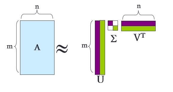
"##  Singular Value Decomposition (SVD)\n",
"---\n",
"* In linear algebra, the singular-value decomposition (SVD) is a factorization of a real or complex matrix. It is the generalization of the eigendecomposition of a positive semidefinite normal matrix (for example, a symmetric matrix with positive eigenvalues) to any $ m\\times n$ matrix via an extension of the polar decomposition.\n",
"* Definition: $$ A_{[m \\times n]} = U_{[m \\times r]} \\Sigma_{[r \\times r]} (V_{[n \\times r]})^T $$"
]
},
{
"cell_type": "markdown",
"metadata": {
"slideshow": {
"slide_type": "subslide"
}
},
"source": [
"* $A$ - Input Data matrix\n",
" * $m \\times n$ matrix (e.g. $m$ documents and $n$ terms that can appear in each document)\n",
"* $U$ - Left Singular vectors\n",
" * $m \\times r$ matrix (e.g. $m$ documents and $r$ concepts)\n",
" * $U = eig(AA^T)$"
]
},
{
"cell_type": "markdown",
"metadata": {
"slideshow": {
"slide_type": "subslide"
}
},
"source": [
"* $\\Sigma$ - Singular values\n",
" * $r \\times r$ **diagonal** matrix (strength of each 'concept')\n",
" * $r$ represnts the **rank** of matrix $A$\n",
" * $\\Sigma = diag\\left(\\sqrt{eigenvalues(A^TA)}\\right)$\n",
" * **Singular Values** definition: the singular values of a matrix $X \\in \\mathbb{R}^{M \\times N}$ are the *square root* of the **eigenvalues** of the matrix $X^TX \\in \\mathbb{R}^{N \\times N}$. If $X \\in \\mathbb{R}^{N \\times N}$ already, then the singular values are the eigenvalues.\n",
"* $V$ - Right Singular vectors\n",
" * $n \\times r$ matrix (e.g. $n$ terms and $r$ concepts)\n",
" * $V = eig(A^TA)$"
]
},
{
"cell_type": "markdown",
"metadata": {
"slideshow": {
"slide_type": "subslide"
}
},
"source": [
"* Illustration:\n",
"
Singular Value Decomposition (SVD)\n",
"---\n",
"* In linear algebra, the singular-value decomposition (SVD) is a factorization of a real or complex matrix. It is the generalization of the eigendecomposition of a positive semidefinite normal matrix (for example, a symmetric matrix with positive eigenvalues) to any $ m\\times n$ matrix via an extension of the polar decomposition.\n",
"* Definition: $$ A_{[m \\times n]} = U_{[m \\times r]} \\Sigma_{[r \\times r]} (V_{[n \\times r]})^T $$"
]
},
{
"cell_type": "markdown",
"metadata": {
"slideshow": {
"slide_type": "subslide"
}
},
"source": [
"* $A$ - Input Data matrix\n",
" * $m \\times n$ matrix (e.g. $m$ documents and $n$ terms that can appear in each document)\n",
"* $U$ - Left Singular vectors\n",
" * $m \\times r$ matrix (e.g. $m$ documents and $r$ concepts)\n",
" * $U = eig(AA^T)$"
]
},
{
"cell_type": "markdown",
"metadata": {
"slideshow": {
"slide_type": "subslide"
}
},
"source": [
"* $\\Sigma$ - Singular values\n",
" * $r \\times r$ **diagonal** matrix (strength of each 'concept')\n",
" * $r$ represnts the **rank** of matrix $A$\n",
" * $\\Sigma = diag\\left(\\sqrt{eigenvalues(A^TA)}\\right)$\n",
" * **Singular Values** definition: the singular values of a matrix $X \\in \\mathbb{R}^{M \\times N}$ are the *square root* of the **eigenvalues** of the matrix $X^TX \\in \\mathbb{R}^{N \\times N}$. If $X \\in \\mathbb{R}^{N \\times N}$ already, then the singular values are the eigenvalues.\n",
"* $V$ - Right Singular vectors\n",
" * $n \\times r$ matrix (e.g. $n$ terms and $r$ concepts)\n",
" * $V = eig(A^TA)$"
]
},
{
"cell_type": "markdown",
"metadata": {
"slideshow": {
"slide_type": "subslide"
}
},
"source": [
"* Illustration:\n",
"  \n",
" First, we see the unit disc in blue together with the two canonical unit vectors. We then see the action of M, which distorts the disk to an ellipse. The SVD decomposes M into three simple transformations: an initial rotation $V^{*}$, a scaling $\\Sigma$ along the coordinate axes, and a final rotation $U$. The lengths $\\sigma_1$ and $\\sigma_2$ of the semi-axes of the ellipse are the singular values of $M$, namely $\\Sigma_{1,1}$ and $\\Sigma_{2,2}$.\n",
" \n",
"* By Kieff - Own work, Public Domain, Link"
]
},
{
"cell_type": "markdown",
"metadata": {
"slideshow": {
"slide_type": "subslide"
}
},
"source": [
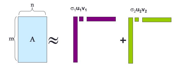
"* Another way to look at SVD: $$ A \\approx U\\Sigma V^T = \\sum_i \\sigma_i u_i \\circ v_i^T $$ \n",
"
\n",
" First, we see the unit disc in blue together with the two canonical unit vectors. We then see the action of M, which distorts the disk to an ellipse. The SVD decomposes M into three simple transformations: an initial rotation $V^{*}$, a scaling $\\Sigma$ along the coordinate axes, and a final rotation $U$. The lengths $\\sigma_1$ and $\\sigma_2$ of the semi-axes of the ellipse are the singular values of $M$, namely $\\Sigma_{1,1}$ and $\\Sigma_{2,2}$.\n",
" \n",
"* By Kieff - Own work, Public Domain, Link"
]
},
{
"cell_type": "markdown",
"metadata": {
"slideshow": {
"slide_type": "subslide"
}
},
"source": [
"* Another way to look at SVD: $$ A \\approx U\\Sigma V^T = \\sum_i \\sigma_i u_i \\circ v_i^T $$ \n",
" 
 "
]
},
{
"cell_type": "markdown",
"metadata": {
"slideshow": {
"slide_type": "subslide"
}
},
"source": [
"* **SVD Properties**\n",
" * It is **always** possible to decompose a **real** matrix $A$ to $A = U\\Sigma V^T$ where\n",
" * $U, \\Sigma, V$ are **uniuqe**\n",
" * $U, V$ are column **orthonormal**\n",
" * $U^T U = I, V^T V = I$\n",
" * $\\Sigma$ is **diagonal**\n",
" * Entries (the singular values) are positive and **sorted** in decreasing order ($\\sigma_1 \\geq \\sigma_2 \\geq ... \\geq 0$)\n",
" * Proof of uniqueness"
]
},
{
"cell_type": "markdown",
"metadata": {
"slideshow": {
"slide_type": "subslide"
}
},
"source": [
"
"
]
},
{
"cell_type": "markdown",
"metadata": {
"slideshow": {
"slide_type": "subslide"
}
},
"source": [
"* **SVD Properties**\n",
" * It is **always** possible to decompose a **real** matrix $A$ to $A = U\\Sigma V^T$ where\n",
" * $U, \\Sigma, V$ are **uniuqe**\n",
" * $U, V$ are column **orthonormal**\n",
" * $U^T U = I, V^T V = I$\n",
" * $\\Sigma$ is **diagonal**\n",
" * Entries (the singular values) are positive and **sorted** in decreasing order ($\\sigma_1 \\geq \\sigma_2 \\geq ... \\geq 0$)\n",
" * Proof of uniqueness"
]
},
{
"cell_type": "markdown",
"metadata": {
"slideshow": {
"slide_type": "subslide"
}
},
"source": [
" \n",
"\n",
"* Image Source"
]
},
{
"cell_type": "markdown",
"metadata": {
"slideshow": {
"slide_type": "slide"
}
},
"source": [
"###
\n",
"\n",
"* Image Source"
]
},
{
"cell_type": "markdown",
"metadata": {
"slideshow": {
"slide_type": "slide"
}
},
"source": [
"###  SVD Example - Users-to-Movies\n",
"---\n",
"We are given a dataset of user's rating (1 to 5) for several movies of 3 genres (concepts) and we wish to use SVD to decompose to the following components:\n",
"* User-to-Concept - which genres the users prefer: $U$ matrix\n",
"* Concepts - what is the strength of each genre in the dataset: $\\Sigma$ - strength of each concept (the singular values)\n",
"* Movie-to-Concept - for each movie, what genres are the most dominant: $V$ matrix"
]
},
{
"cell_type": "code",
"execution_count": 17,
"metadata": {
"slideshow": {
"slide_type": "subslide"
}
},
"outputs": [
{
"name": "stdout",
"output_type": "stream",
"text": [
"User-to-Movies matrix:\n"
]
},
{
"data": {
"text/html": [
"
SVD Example - Users-to-Movies\n",
"---\n",
"We are given a dataset of user's rating (1 to 5) for several movies of 3 genres (concepts) and we wish to use SVD to decompose to the following components:\n",
"* User-to-Concept - which genres the users prefer: $U$ matrix\n",
"* Concepts - what is the strength of each genre in the dataset: $\\Sigma$ - strength of each concept (the singular values)\n",
"* Movie-to-Concept - for each movie, what genres are the most dominant: $V$ matrix"
]
},
{
"cell_type": "code",
"execution_count": 17,
"metadata": {
"slideshow": {
"slide_type": "subslide"
}
},
"outputs": [
{
"name": "stdout",
"output_type": "stream",
"text": [
"User-to-Movies matrix:\n"
]
},
{
"data": {
"text/html": [
"\n",
"\n",
"
\n",
" \n",
" \n",
" | \n",
" Matrix | \n",
" Alien | \n",
" Serenity | \n",
" Casablanca | \n",
" Amelie | \n",
"
\n",
" \n",
" \n",
" \n",
" | User 1 | \n",
" 1 | \n",
" 1 | \n",
" 1 | \n",
" 0 | \n",
" 0 | \n",
"
\n",
" \n",
" | User 2 | \n",
" 3 | \n",
" 3 | \n",
" 3 | \n",
" 0 | \n",
" 0 | \n",
"
\n",
" \n",
" | User 3 | \n",
" 4 | \n",
" 4 | \n",
" 4 | \n",
" 0 | \n",
" 0 | \n",
"
\n",
" \n",
" | User 4 | \n",
" 5 | \n",
" 5 | \n",
" 5 | \n",
" 0 | \n",
" 0 | \n",
"
\n",
" \n",
" | User 5 | \n",
" 0 | \n",
" 2 | \n",
" 0 | \n",
" 4 | \n",
" 4 | \n",
"
\n",
" \n",
" | User 6 | \n",
" 0 | \n",
" 0 | \n",
" 0 | \n",
" 5 | \n",
" 5 | \n",
"
\n",
" \n",
" | User 7 | \n",
" 0 | \n",
" 1 | \n",
" 0 | \n",
" 2 | \n",
" 2 | \n",
"
\n",
" \n",
"
\n",
"
\n",
"\n",
"
\n",
" \n",
" \n",
" | \n",
" Matrix | \n",
" Alien | \n",
" Serenity | \n",
" Casablanca | \n",
" Amelie | \n",
"
\n",
" \n",
" \n",
" \n",
" | User 1 | \n",
" 1.0 | \n",
" 1.0 | \n",
" 1.0 | \n",
" 0.0 | \n",
" 0.0 | \n",
"
\n",
" \n",
" | User 2 | \n",
" 3.0 | \n",
" 3.0 | \n",
" 3.0 | \n",
" -0.0 | \n",
" -0.0 | \n",
"
\n",
" \n",
" | User 3 | \n",
" 4.0 | \n",
" 4.0 | \n",
" 4.0 | \n",
" 0.0 | \n",
" -0.0 | \n",
"
\n",
" \n",
" | User 4 | \n",
" 5.0 | \n",
" 5.0 | \n",
" 5.0 | \n",
" -0.0 | \n",
" -0.0 | \n",
"
\n",
" \n",
" | User 5 | \n",
" 0.0 | \n",
" 2.0 | \n",
" -0.0 | \n",
" 4.0 | \n",
" 4.0 | \n",
"
\n",
" \n",
" | User 6 | \n",
" 0.0 | \n",
" 0.0 | \n",
" -0.0 | \n",
" 5.0 | \n",
" 5.0 | \n",
"
\n",
" \n",
" | User 7 | \n",
" 0.0 | \n",
" 1.0 | \n",
" -0.0 | \n",
" 2.0 | \n",
" 2.0 | \n",
"
\n",
" \n",
"
\n",
"
 "
]
},
{
"cell_type": "markdown",
"metadata": {
"slideshow": {
"slide_type": "slide"
}
},
"source": [
"###
"
]
},
{
"cell_type": "markdown",
"metadata": {
"slideshow": {
"slide_type": "slide"
}
},
"source": [
"###  Recommended Videos\n",
"---\n",
"####
Recommended Videos\n",
"---\n",
"####  Warning!\n",
"* These videos do not replace the lectures and tutorials.\n",
"* Please use these to get a better understanding of the material, and not as an alternative to the written material.\n",
"\n",
"#### Video By Subject\n",
"* Basic Linear Algebra - Mathematics for Machine Learning full Course || Linear Algebra || Part-1\n",
"* SVD - Lecture 47 — Singular Value Decomposition | Stanford University\n"
]
},
{
"cell_type": "markdown",
"metadata": {
"slideshow": {
"slide_type": "skip"
}
},
"source": [
"##
Warning!\n",
"* These videos do not replace the lectures and tutorials.\n",
"* Please use these to get a better understanding of the material, and not as an alternative to the written material.\n",
"\n",
"#### Video By Subject\n",
"* Basic Linear Algebra - Mathematics for Machine Learning full Course || Linear Algebra || Part-1\n",
"* SVD - Lecture 47 — Singular Value Decomposition | Stanford University\n"
]
},
{
"cell_type": "markdown",
"metadata": {
"slideshow": {
"slide_type": "skip"
}
},
"source": [
"##  Credits\n",
"---\n",
"* Inspired by slides by Elad Osherov and slides from MMDS\n",
"* Icons from Icon8.com - https://icons8.com\n",
"* Datasets from Kaggle - https://www.kaggle.com/"
]
}
],
"metadata": {
"kernelspec": {
"display_name": "Python 3",
"language": "python",
"name": "python3"
},
"language_info": {
"codemirror_mode": {
"name": "ipython",
"version": 3
},
"file_extension": ".py",
"mimetype": "text/x-python",
"name": "python",
"nbconvert_exporter": "python",
"pygments_lexer": "ipython3",
"version": "3.6.9"
}
},
"nbformat": 4,
"nbformat_minor": 2
}
Credits\n",
"---\n",
"* Inspired by slides by Elad Osherov and slides from MMDS\n",
"* Icons from Icon8.com - https://icons8.com\n",
"* Datasets from Kaggle - https://www.kaggle.com/"
]
}
],
"metadata": {
"kernelspec": {
"display_name": "Python 3",
"language": "python",
"name": "python3"
},
"language_info": {
"codemirror_mode": {
"name": "ipython",
"version": 3
},
"file_extension": ".py",
"mimetype": "text/x-python",
"name": "python",
"nbconvert_exporter": "python",
"pygments_lexer": "ipython3",
"version": "3.6.9"
}
},
"nbformat": 4,
"nbformat_minor": 2
}
\")