 CS 236756 - Technion - Intro to Machine Learning\n",
"---\n",
"#### Tal Daniel\n",
"\n",
"\n",
"## Tutorial 06 - Decision Trees\n",
"---"
]
},
{
"cell_type": "markdown",
"metadata": {
"slideshow": {
"slide_type": "slide"
}
},
"source": [
"###
CS 236756 - Technion - Intro to Machine Learning\n",
"---\n",
"#### Tal Daniel\n",
"\n",
"\n",
"## Tutorial 06 - Decision Trees\n",
"---"
]
},
{
"cell_type": "markdown",
"metadata": {
"slideshow": {
"slide_type": "slide"
}
},
"source": [
"###  Agenda\n",
"---\n",
"\n",
"* [Motivation](#-Motivation)\n",
"* [How Decision Trees Work](#-Considerations-for-Building-a-Tree)\n",
"* [Decision Boundries](#-Decision-Boundries-(Also-for-Regression-Tasks) )\n",
"* [Impurity Metrics](#-Impurity-&-Impurity-Metrics)\n",
" * [Entropy](#Entropy)\n",
" * [Gini](#Gini-Index)\n",
"* [Relation Mutual Information (Information Gain)](#Relation-Mutual-Information-(Information-Gain) )\n",
"* [Prunning & Regularization](#-Prunning-&-Regularization-Hyperparameters)\n",
"* [Example on the Titanic Dataset](#-Example---Titanic-Dataset)\n",
"* [Random Forest](#-Random-Forest)\n",
"* [Recommended Videos](#-Recommended-Videos)\n",
"* [Credits](#-Credits)"
]
},
{
"cell_type": "code",
"execution_count": 1,
"metadata": {
"slideshow": {
"slide_type": "skip"
}
},
"outputs": [],
"source": [
"# imports for the tutorial\n",
"import numpy as np\n",
"import pandas as pd\n",
"import re # regex\n",
"from sklearn.tree import DecisionTreeClassifier\n",
"import matplotlib.pyplot as plt\n",
"%matplotlib notebook"
]
},
{
"cell_type": "markdown",
"metadata": {
"slideshow": {
"slide_type": "slide"
}
},
"source": [
"##
Agenda\n",
"---\n",
"\n",
"* [Motivation](#-Motivation)\n",
"* [How Decision Trees Work](#-Considerations-for-Building-a-Tree)\n",
"* [Decision Boundries](#-Decision-Boundries-(Also-for-Regression-Tasks) )\n",
"* [Impurity Metrics](#-Impurity-&-Impurity-Metrics)\n",
" * [Entropy](#Entropy)\n",
" * [Gini](#Gini-Index)\n",
"* [Relation Mutual Information (Information Gain)](#Relation-Mutual-Information-(Information-Gain) )\n",
"* [Prunning & Regularization](#-Prunning-&-Regularization-Hyperparameters)\n",
"* [Example on the Titanic Dataset](#-Example---Titanic-Dataset)\n",
"* [Random Forest](#-Random-Forest)\n",
"* [Recommended Videos](#-Recommended-Videos)\n",
"* [Credits](#-Credits)"
]
},
{
"cell_type": "code",
"execution_count": 1,
"metadata": {
"slideshow": {
"slide_type": "skip"
}
},
"outputs": [],
"source": [
"# imports for the tutorial\n",
"import numpy as np\n",
"import pandas as pd\n",
"import re # regex\n",
"from sklearn.tree import DecisionTreeClassifier\n",
"import matplotlib.pyplot as plt\n",
"%matplotlib notebook"
]
},
{
"cell_type": "markdown",
"metadata": {
"slideshow": {
"slide_type": "slide"
}
},
"source": [
"##  Motivation\n",
"---\n",
"* Decision Trees are ML algorithms that can perform **both** classification and regression tasks, and even multioutput tasks.\n",
"* They are very powerful algorithms, capable of fitting complex datasets.\n",
"* They are a fundamental component of **Random Forests**, which are amongst the most powerful ML algorithms today. \n",
"* Decision Trees require **very little data** preparation - they do not require **feature scaling or centering**."
]
},
{
"cell_type": "markdown",
"metadata": {
"slideshow": {
"slide_type": "slide"
}
},
"source": [
"###
Motivation\n",
"---\n",
"* Decision Trees are ML algorithms that can perform **both** classification and regression tasks, and even multioutput tasks.\n",
"* They are very powerful algorithms, capable of fitting complex datasets.\n",
"* They are a fundamental component of **Random Forests**, which are amongst the most powerful ML algorithms today. \n",
"* Decision Trees require **very little data** preparation - they do not require **feature scaling or centering**."
]
},
{
"cell_type": "markdown",
"metadata": {
"slideshow": {
"slide_type": "slide"
}
},
"source": [
"###  Examples\n",
"---\n",
"
Examples\n",
"---\n",
" "
]
},
{
"cell_type": "markdown",
"metadata": {
"slideshow": {
"slide_type": "subslide"
}
},
"source": [
"**20 Questions** - one player is chosen to be the answerer. That person chooses a subject (object) but does not reveal this to the others. All other players are questioners. They each take turns asking a question which can be answered with a simple \"Yes\" or \"No.\"\n",
"* *Features* - different properties of a character we ask about\n",
"* *Label* - the identity of the character\n",
"* *Training Set* - the characters you have encountered in your life\n",
"* *Test/Inference* - play \"20 Questions\"\n",
"* A good strategy:\n",
" * Eliminate as many options as possible\n",
" * Simple questions\n",
" * Consider more likely characters (Leibniz isn't who most people think of, but in the Technion, this might not be the case...)\n",
"* Note: this game is a special case of classification where *each sample is its own class*"
]
},
{
"cell_type": "markdown",
"metadata": {
"slideshow": {
"slide_type": "slide"
}
},
"source": [
"###
"
]
},
{
"cell_type": "markdown",
"metadata": {
"slideshow": {
"slide_type": "subslide"
}
},
"source": [
"**20 Questions** - one player is chosen to be the answerer. That person chooses a subject (object) but does not reveal this to the others. All other players are questioners. They each take turns asking a question which can be answered with a simple \"Yes\" or \"No.\"\n",
"* *Features* - different properties of a character we ask about\n",
"* *Label* - the identity of the character\n",
"* *Training Set* - the characters you have encountered in your life\n",
"* *Test/Inference* - play \"20 Questions\"\n",
"* A good strategy:\n",
" * Eliminate as many options as possible\n",
" * Simple questions\n",
" * Consider more likely characters (Leibniz isn't who most people think of, but in the Technion, this might not be the case...)\n",
"* Note: this game is a special case of classification where *each sample is its own class*"
]
},
{
"cell_type": "markdown",
"metadata": {
"slideshow": {
"slide_type": "slide"
}
},
"source": [
"###  Decision Tree Visualization\n",
"---\n",
"
Decision Tree Visualization\n",
"---\n",
" "
]
},
{
"cell_type": "markdown",
"metadata": {},
"source": [
"###
"
]
},
{
"cell_type": "markdown",
"metadata": {},
"source": [
"###  Considerations for Building a Tree\n",
"---\n",
"#### **Binary** or **Multi-Valued**\n",
"* Each split can be into 2 nodes or more than 2 nodes. Binary trees are easier to work with.\n",
"* Every *Polythetic* tree can be represented by an equivalent *Monothetic* tree.\n",
"* For example, the following tree can be transformed to the tree in the previous section:
Considerations for Building a Tree\n",
"---\n",
"#### **Binary** or **Multi-Valued**\n",
"* Each split can be into 2 nodes or more than 2 nodes. Binary trees are easier to work with.\n",
"* Every *Polythetic* tree can be represented by an equivalent *Monothetic* tree.\n",
"* For example, the following tree can be transformed to the tree in the previous section: 
 Decision Boundaries (Also for Regression Tasks)\n",
"---\n",
"* In regression problems, the data is continuous, and boundaries have to be set such that the input falls within a certain range.\n",
"* These decision boundaries can easily drawn on a graph as in the following example:
Decision Boundaries (Also for Regression Tasks)\n",
"---\n",
"* In regression problems, the data is continuous, and boundaries have to be set such that the input falls within a certain range.\n",
"* These decision boundaries can easily drawn on a graph as in the following example:  "
]
},
{
"cell_type": "markdown",
"metadata": {
"slideshow": {
"slide_type": "subslide"
}
},
"source": [
"####
"
]
},
{
"cell_type": "markdown",
"metadata": {
"slideshow": {
"slide_type": "subslide"
}
},
"source": [
"####  Decision Trees for Regression Tasks\n",
"---\n",
"* In this tutorial we deal with classification tasks, where the input can be continuous features, but what if we want to complete a regression task, that is, output a value and not a class?\n",
"\n",
"* Decision Trees are also capable of performing these tasks. We will not get into it, but the idea is the same. \n",
"* Instead of predicting a class, the tree predicts a value which is determined by the mean of the values in that branch.\n",
"* The CART algorithm is almost the same except for instead of minimizing the impurity, the MSE is minimized. \n",
"* You can read more about it on Scikit-Learn's documentation, under `DecisionTreeRegressor`."
]
},
{
"cell_type": "markdown",
"metadata": {
"slideshow": {
"slide_type": "slide"
}
},
"source": [
"###
Decision Trees for Regression Tasks\n",
"---\n",
"* In this tutorial we deal with classification tasks, where the input can be continuous features, but what if we want to complete a regression task, that is, output a value and not a class?\n",
"\n",
"* Decision Trees are also capable of performing these tasks. We will not get into it, but the idea is the same. \n",
"* Instead of predicting a class, the tree predicts a value which is determined by the mean of the values in that branch.\n",
"* The CART algorithm is almost the same except for instead of minimizing the impurity, the MSE is minimized. \n",
"* You can read more about it on Scikit-Learn's documentation, under `DecisionTreeRegressor`."
]
},
{
"cell_type": "markdown",
"metadata": {
"slideshow": {
"slide_type": "slide"
}
},
"source": [
"###  Estimating Class Probabilities (Class Conditional Probabality)\n",
"---\n",
"* A Decision Tree can also estimate the probability that an instance belongs to a particular class $k$\n",
" * First, it traverses the tree to find the leaf node for this instance\n",
" * Then, it returns the ratio of *training* instances of class $k$ in this node\n",
" * In Scikit-Learn (after training) - `tree_clf.predict_proba([list of samples])`\n",
"* The class-conditional probabilities $P(c|D)$ are estimated by fitting a categorical MLE: $$ p_i = P(c|D) = \\frac{1}{|D|} \\sum_{i \\in D} \\mathbb{1}(y_i =c) $$\n",
" * $c$ - class\n",
" * $D$ - Data\n",
" * Reminder - **Categorical Distribution** is a generalization of Bernoulli to multiple classes"
]
},
{
"cell_type": "markdown",
"metadata": {
"slideshow": {
"slide_type": "slide"
}
},
"source": [
"##
Estimating Class Probabilities (Class Conditional Probabality)\n",
"---\n",
"* A Decision Tree can also estimate the probability that an instance belongs to a particular class $k$\n",
" * First, it traverses the tree to find the leaf node for this instance\n",
" * Then, it returns the ratio of *training* instances of class $k$ in this node\n",
" * In Scikit-Learn (after training) - `tree_clf.predict_proba([list of samples])`\n",
"* The class-conditional probabilities $P(c|D)$ are estimated by fitting a categorical MLE: $$ p_i = P(c|D) = \\frac{1}{|D|} \\sum_{i \\in D} \\mathbb{1}(y_i =c) $$\n",
" * $c$ - class\n",
" * $D$ - Data\n",
" * Reminder - **Categorical Distribution** is a generalization of Bernoulli to multiple classes"
]
},
{
"cell_type": "markdown",
"metadata": {
"slideshow": {
"slide_type": "slide"
}
},
"source": [
"##  Impurity & Impurity Metrics\n",
"---\n",
"* **Simplicity** is the leading principle in the tree building process\n",
"* Therefore, we seek an attribute $A$ at each node $S$ that makes the immediate descendents as \"pure\" as possible.\n",
"* At each node $S$, the vector $P=(p_1, p_2, ..., p_k)$, represents the probability (ratio) of samples belonging to class $i$\n",
" * **Impurity** of node $S$ - $\\phi(P) \\geq 0$\n",
" * $\\phi(P)=0$ if all samples have the same label\n",
" * That is, a node is \"pure\" if all training instances it applies to belong to the same class\n",
" * $\\phi(P)$ is *maximized* for **uniform distribution**\n",
" * $\\phi(P)$ is **symmetric** w.r.t. $P$\n",
" * $\\phi(P)$ is *smooth*, that is, differentiable everywhere"
]
},
{
"cell_type": "markdown",
"metadata": {
"slideshow": {
"slide_type": "slide"
}
},
"source": [
"###
Impurity & Impurity Metrics\n",
"---\n",
"* **Simplicity** is the leading principle in the tree building process\n",
"* Therefore, we seek an attribute $A$ at each node $S$ that makes the immediate descendents as \"pure\" as possible.\n",
"* At each node $S$, the vector $P=(p_1, p_2, ..., p_k)$, represents the probability (ratio) of samples belonging to class $i$\n",
" * **Impurity** of node $S$ - $\\phi(P) \\geq 0$\n",
" * $\\phi(P)=0$ if all samples have the same label\n",
" * That is, a node is \"pure\" if all training instances it applies to belong to the same class\n",
" * $\\phi(P)$ is *maximized* for **uniform distribution**\n",
" * $\\phi(P)$ is **symmetric** w.r.t. $P$\n",
" * $\\phi(P)$ is *smooth*, that is, differentiable everywhere"
]
},
{
"cell_type": "markdown",
"metadata": {
"slideshow": {
"slide_type": "slide"
}
},
"source": [
"###  Impurity Metrics\n",
"---\n",
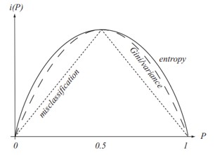
"#### Entropy\n",
"---\n",
"* The concept of entropy originates in thermodynamics as a measure of *molecular disorder*. Entropy approaches 0 when molecules are still and well ordered.\n",
"* Later, it was introduced in the *information theory* domain, where the average information content of a message is measured (a reduction in entropy is called **information gain**). When all messages are identical, the entropy is zero.\n",
"* In Machine Learning, it is used as an impurity measure - a set's entropy is 0 when it contains instances of only one class.\n",
"* Given a system whose exact description is *unknown*, its entropy is defined as **the amount of information needed to exactly specify the state of the system**\n",
" * If the system has $k$ states, we would need $\\log k$ bits to represent them"
]
},
{
"cell_type": "markdown",
"metadata": {
"slideshow": {
"slide_type": "subslide"
}
},
"source": [
"* Denote $p_{i, k}$ as the ratio of class $k$ instances among the training instances in the $i^{th}$ node, the entropy is: $$ H_i = \\sum_{k=1}^n p_{i,k} \\log\\frac{1}{p_{i,k}} = - \\sum_{k=1}^n p_{i,k} \\log p_{i,k} $$\n",
"*
Impurity Metrics\n",
"---\n",
"#### Entropy\n",
"---\n",
"* The concept of entropy originates in thermodynamics as a measure of *molecular disorder*. Entropy approaches 0 when molecules are still and well ordered.\n",
"* Later, it was introduced in the *information theory* domain, where the average information content of a message is measured (a reduction in entropy is called **information gain**). When all messages are identical, the entropy is zero.\n",
"* In Machine Learning, it is used as an impurity measure - a set's entropy is 0 when it contains instances of only one class.\n",
"* Given a system whose exact description is *unknown*, its entropy is defined as **the amount of information needed to exactly specify the state of the system**\n",
" * If the system has $k$ states, we would need $\\log k$ bits to represent them"
]
},
{
"cell_type": "markdown",
"metadata": {
"slideshow": {
"slide_type": "subslide"
}
},
"source": [
"* Denote $p_{i, k}$ as the ratio of class $k$ instances among the training instances in the $i^{th}$ node, the entropy is: $$ H_i = \\sum_{k=1}^n p_{i,k} \\log\\frac{1}{p_{i,k}} = - \\sum_{k=1}^n p_{i,k} \\log p_{i,k} $$\n",
"*  "
]
},
{
"cell_type": "markdown",
"metadata": {
"slideshow": {
"slide_type": "subslide"
}
},
"source": [
"#### Gini Index\n",
"---\n",
"* Gini is another common measure for impurity which can be intepreted as a *variance impurity*\n",
"* Denote $p_{i, k}$ as the ratio of class $k$ instances among the training instances in the $i^{th}$ node, the GiniIndex is: $$ G_i(P) = \\sum_{k=1}^n p_{i,k} (1-p_{i,k}) = 1 - \\sum_{k=1}^n p_{i,k}^2 $$\n",
" * Reminder: given $X \\sim Bern(p) \\rightarrow Var(X) = p \\cdot (1-p)$\n",
"* This is the expected error rate at node $N$ if the category label is selected randomly from class distribution present at $N$\n",
"\n",
"
"
]
},
{
"cell_type": "markdown",
"metadata": {
"slideshow": {
"slide_type": "subslide"
}
},
"source": [
"#### Gini Index\n",
"---\n",
"* Gini is another common measure for impurity which can be intepreted as a *variance impurity*\n",
"* Denote $p_{i, k}$ as the ratio of class $k$ instances among the training instances in the $i^{th}$ node, the GiniIndex is: $$ G_i(P) = \\sum_{k=1}^n p_{i,k} (1-p_{i,k}) = 1 - \\sum_{k=1}^n p_{i,k}^2 $$\n",
" * Reminder: given $X \\sim Bern(p) \\rightarrow Var(X) = p \\cdot (1-p)$\n",
"* This is the expected error rate at node $N$ if the category label is selected randomly from class distribution present at $N$\n",
"\n",
" "
]
},
{
"cell_type": "markdown",
"metadata": {
"slideshow": {
"slide_type": "slide"
}
},
"source": [
"#### Gini vs. Entropy\n",
"---\n",
"* Scikit-Learn's default is **Gini**, but by changing the call to `criterion=\"entropy\"`, the Entropy will be used to build the tree\n",
"* Most of the time, **both** lead to similar trees.\n",
"* **Gini** is (slightly) faster to compute\n",
"* However, sometimes they are different as Gini tends to isloate the most frequent class in its own branch of the tree, while Entropy tends to produce slightly more *balanced* trees"
]
},
{
"cell_type": "markdown",
"metadata": {
"slideshow": {
"slide_type": "slide"
}
},
"source": [
"##
"
]
},
{
"cell_type": "markdown",
"metadata": {
"slideshow": {
"slide_type": "slide"
}
},
"source": [
"#### Gini vs. Entropy\n",
"---\n",
"* Scikit-Learn's default is **Gini**, but by changing the call to `criterion=\"entropy\"`, the Entropy will be used to build the tree\n",
"* Most of the time, **both** lead to similar trees.\n",
"* **Gini** is (slightly) faster to compute\n",
"* However, sometimes they are different as Gini tends to isloate the most frequent class in its own branch of the tree, while Entropy tends to produce slightly more *balanced* trees"
]
},
{
"cell_type": "markdown",
"metadata": {
"slideshow": {
"slide_type": "slide"
}
},
"source": [
"##  Choosing the Features/Attributes for the Splits\n",
"---\n",
"* Choose the one that most decreases impurity (and thus, increases purity)\n",
"* Given node $S$ with probabilities $P$ and discrete attribute $A$, the **impurity drop** is defined as: $$ \\Delta \\phi(S,A) = \\phi(S) - \\sum_{v \\in \\textit{Values}(A)} p_v \\phi(S_v) $$\n",
" * For the **Binary** case: $$ \\Delta \\phi(S,A) = \\phi(S) - p_L \\phi(S_L) - (1 - p_L) \\phi(S_R) $$\n",
"* For the *Entropy* measure, this measure is called **Information Gain (IG)** (or Mutual Information - MI): $$ IG(P) = H(P) - \\sum_{v \\in \\textit{Values}(A)} p_aH(p_a)$$\n",
"* For *Gini*, the measure is called **Gini Gain**"
]
},
{
"cell_type": "markdown",
"metadata": {
"slideshow": {
"slide_type": "subslide"
}
},
"source": [
"* We wish to **maximize** the information gain on the impurity drop, which is equivalent to **minimizing** the right expression.\n",
"* Denote a single feature as $k$ and a threshold value as $t_k$ (for example, height $\\leq 30 $ cm) ,**the CART algorithm cost function** (which we wish to minimize): $$ J(k, t_k) = \\frac{m_{left}}{m}G_{left} + \\frac{m_{right}}{m}G_{right} = p_LG_{left} + p_R G_{right} $$ where $G_{left/right}$ is the measure of impurity of the left/right subset and $m_{left/right}$ is the number of instances in the left/right subset.\n",
"* The tree building algorithm (CART) is *greedy*, it greedily searches for an optimum split at the top level, then repeats the process at each level. It does not check whether or not the split will lead to the lowest possible impurity several levels down. A greedy algorithm usually produces reasonably good solutions, but they are not guaranteed to be optimal. "
]
},
{
"cell_type": "markdown",
"metadata": {
"slideshow": {
"slide_type": "slide"
}
},
"source": [
"###
Choosing the Features/Attributes for the Splits\n",
"---\n",
"* Choose the one that most decreases impurity (and thus, increases purity)\n",
"* Given node $S$ with probabilities $P$ and discrete attribute $A$, the **impurity drop** is defined as: $$ \\Delta \\phi(S,A) = \\phi(S) - \\sum_{v \\in \\textit{Values}(A)} p_v \\phi(S_v) $$\n",
" * For the **Binary** case: $$ \\Delta \\phi(S,A) = \\phi(S) - p_L \\phi(S_L) - (1 - p_L) \\phi(S_R) $$\n",
"* For the *Entropy* measure, this measure is called **Information Gain (IG)** (or Mutual Information - MI): $$ IG(P) = H(P) - \\sum_{v \\in \\textit{Values}(A)} p_aH(p_a)$$\n",
"* For *Gini*, the measure is called **Gini Gain**"
]
},
{
"cell_type": "markdown",
"metadata": {
"slideshow": {
"slide_type": "subslide"
}
},
"source": [
"* We wish to **maximize** the information gain on the impurity drop, which is equivalent to **minimizing** the right expression.\n",
"* Denote a single feature as $k$ and a threshold value as $t_k$ (for example, height $\\leq 30 $ cm) ,**the CART algorithm cost function** (which we wish to minimize): $$ J(k, t_k) = \\frac{m_{left}}{m}G_{left} + \\frac{m_{right}}{m}G_{right} = p_LG_{left} + p_R G_{right} $$ where $G_{left/right}$ is the measure of impurity of the left/right subset and $m_{left/right}$ is the number of instances in the left/right subset.\n",
"* The tree building algorithm (CART) is *greedy*, it greedily searches for an optimum split at the top level, then repeats the process at each level. It does not check whether or not the split will lead to the lowest possible impurity several levels down. A greedy algorithm usually produces reasonably good solutions, but they are not guaranteed to be optimal. "
]
},
{
"cell_type": "markdown",
"metadata": {
"slideshow": {
"slide_type": "slide"
}
},
"source": [
"###  Relation to Mutual Information (Information Gain)\n",
"---\n",
"\n",
"* **Mutual Information (MI)** calculates the statistical dependence between two variables and is the name given to information gain when applied to variable selection.\n",
"* MI is calculated between two variables and measures the reduction in uncertainty for one variable given a known value of the other variable.\n",
"* The mutual information between two random variables X and Y can be stated formally as follows: $$ I(X;Y) = H(X) - H(X \\mid Y) $$\n",
" * $I(X ; Y)$ is the mutual information for $X$ and $Y$, $H(X)$ is the entropy for $X$ and $H(X \\mid Y)$ is the conditional entropy for $X$ given $Y$. \n",
" * The result has the units of *bits*.\n",
"* MI is always **larger than or equal to zero**, where the larger the value, the greater the relationship between the two variables. If the calculated result is zero, then the variables are **independent**."
]
},
{
"cell_type": "markdown",
"metadata": {
"slideshow": {
"slide_type": "subslide"
}
},
"source": [
"* Mutual Information and Information Gain are the same thing, although the context or usage of the measure often gives rise to the different names. For example:\n",
" * Effect of Transforms to a Dataset (Decision Trees): Information Gain.\n",
" * Dependence Between Variables (Feature Selection): Mutual Information.\n",
"* Notice the similarity in the way that the mutual information is calculated and the way that information gain is calculated, they are equivalent: $$I(X;Y) = H(X) - H(X \\mid Y) $$ $$ IG(S, a) = H(S) - H(S \\mid a)$$"
]
},
{
"cell_type": "markdown",
"metadata": {
"slideshow": {
"slide_type": "slide"
}
},
"source": [
"####
Relation to Mutual Information (Information Gain)\n",
"---\n",
"\n",
"* **Mutual Information (MI)** calculates the statistical dependence between two variables and is the name given to information gain when applied to variable selection.\n",
"* MI is calculated between two variables and measures the reduction in uncertainty for one variable given a known value of the other variable.\n",
"* The mutual information between two random variables X and Y can be stated formally as follows: $$ I(X;Y) = H(X) - H(X \\mid Y) $$\n",
" * $I(X ; Y)$ is the mutual information for $X$ and $Y$, $H(X)$ is the entropy for $X$ and $H(X \\mid Y)$ is the conditional entropy for $X$ given $Y$. \n",
" * The result has the units of *bits*.\n",
"* MI is always **larger than or equal to zero**, where the larger the value, the greater the relationship between the two variables. If the calculated result is zero, then the variables are **independent**."
]
},
{
"cell_type": "markdown",
"metadata": {
"slideshow": {
"slide_type": "subslide"
}
},
"source": [
"* Mutual Information and Information Gain are the same thing, although the context or usage of the measure often gives rise to the different names. For example:\n",
" * Effect of Transforms to a Dataset (Decision Trees): Information Gain.\n",
" * Dependence Between Variables (Feature Selection): Mutual Information.\n",
"* Notice the similarity in the way that the mutual information is calculated and the way that information gain is calculated, they are equivalent: $$I(X;Y) = H(X) - H(X \\mid Y) $$ $$ IG(S, a) = H(S) - H(S \\mid a)$$"
]
},
{
"cell_type": "markdown",
"metadata": {
"slideshow": {
"slide_type": "slide"
}
},
"source": [
"####  Exercise 1 - Decsion Tree by Hand\n",
"---\n",
"As of September 2012, 800 extrasolar planets have been identified in our galaxy. Supersecret surveying spaceships sent to all these planets have established whether they are habitable for humans or not, but sending a spaceship to each planet is expensive. In this problem, you will come up with decision trees to predict if a planet is habitable\n",
"based only on features observable using telescopes.\n",
"\n",
"In the following table you are given the data from all 800 planets surveyed so far. The features observed by telescope are Size (“Big” or “Small”), and Orbit (“Near” or “Far”). Each row indicates the values of the features and habitability, and how many times that set of values was observed. So, for example, there were 20 “Big” planets “Near” their star that\n",
"were habitable."
]
},
{
"cell_type": "markdown",
"metadata": {
"slideshow": {
"slide_type": "subslide"
}
},
"source": [
"|
Exercise 1 - Decsion Tree by Hand\n",
"---\n",
"As of September 2012, 800 extrasolar planets have been identified in our galaxy. Supersecret surveying spaceships sent to all these planets have established whether they are habitable for humans or not, but sending a spaceship to each planet is expensive. In this problem, you will come up with decision trees to predict if a planet is habitable\n",
"based only on features observable using telescopes.\n",
"\n",
"In the following table you are given the data from all 800 planets surveyed so far. The features observed by telescope are Size (“Big” or “Small”), and Orbit (“Near” or “Far”). Each row indicates the values of the features and habitability, and how many times that set of values was observed. So, for example, there were 20 “Big” planets “Near” their star that\n",
"were habitable."
]
},
{
"cell_type": "markdown",
"metadata": {
"slideshow": {
"slide_type": "subslide"
}
},
"source": [
"|  Solution 1\n",
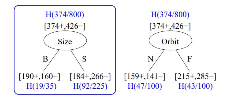
"Let's first calculate the entropy of starting state: $$ H(Habitable) = -\\frac{20 + 170 + 139+45}{800} \\log_2 \\frac{20 + 170 + 139+45}{800} -\\frac{130 + 30 + 11+255}{800} \\log_2 \\frac{130 + 30 + 11+255}{800}$$
Solution 1\n",
"Let's first calculate the entropy of starting state: $$ H(Habitable) = -\\frac{20 + 170 + 139+45}{800} \\log_2 \\frac{20 + 170 + 139+45}{800} -\\frac{130 + 30 + 11+255}{800} \\log_2 \\frac{130 + 30 + 11+255}{800}$$ $$ = -\\frac{374}{800} \\log_2 \\frac{374}{800} -\\frac{426}{800} \\log_2 \\frac{426}{800} = 0.4841 + 0.5183 \\approx 1 $$\n", "\n", "Let's calculate the **Information Gain** from each split:\n", "$$ H(Habitable|Size) = \\frac{190+160}{800}H(Size=Big) + \\frac{184+266}{800}H(Size=Small) $$
$$ = \\frac{350}{800} \\cdot (-\\frac{190}{350}\\log_2 (\\frac{190}{350}) -\\frac{160}{350}\\log_2 (\\frac{160}{350})) + \\frac{450}{800}\\cdot(-\\frac{184}{450}\\log_2 (\\frac{184}{450}) -\\frac{266}{450}\\log_2 (\\frac{266}{450}))$$
$$ = 0.984 \\rightarrow IG(Habitable|Size) = 1 - 0.984 = 0.016 $$" ] }, { "cell_type": "markdown", "metadata": { "slideshow": { "slide_type": "subslide" } }, "source": [ "$$ H(Habitable|Orbit) = \\frac{159+141}{800}H(Orbit=Near) + \\frac{215 + 285}{800}H(Orbit=Far) $$
$$ = \\frac{300}{800} \\cdot (-\\frac{159}{300}\\log_2 (\\frac{159}{300}) -\\frac{141}{300}\\log_2 (\\frac{141}{300})) + \\frac{500}{800}\\cdot(-\\frac{215}{500}\\log_2 (\\frac{215}{500}) -\\frac{285}{500}\\log_2 (\\frac{282}{500})) $$
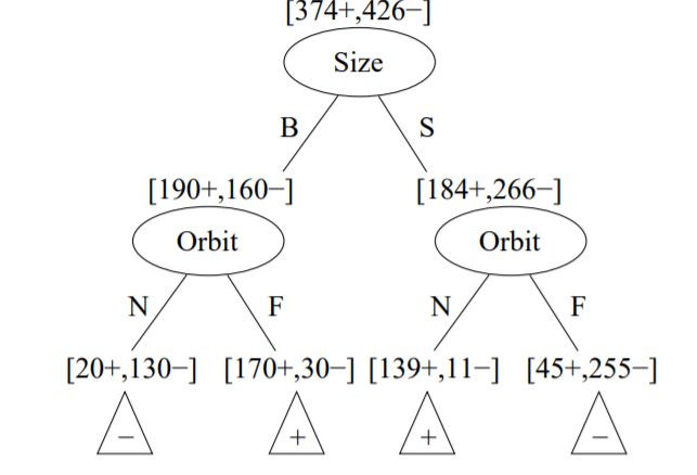
$$ = 0.9901 \\rightarrow IG(Habitable|Orbit) = 1 - 0.9901 = 0.009 $$" ] }, { "cell_type": "markdown", "metadata": { "slideshow": { "slide_type": "subslide" } }, "source": [ "So the Information Gain from the size is larger, thus, the first split will be based on the Size feature.\n", "
 "
]
},
{
"cell_type": "markdown",
"metadata": {
"slideshow": {
"slide_type": "subslide"
}
},
"source": [
"The final tree looks like this:\n",
"
"
]
},
{
"cell_type": "markdown",
"metadata": {
"slideshow": {
"slide_type": "subslide"
}
},
"source": [
"The final tree looks like this:\n",
" \n",
"\n",
"#### More Decision Trees Practice Excercises "
]
},
{
"cell_type": "markdown",
"metadata": {
"slideshow": {
"slide_type": "slide"
}
},
"source": [
"###
\n",
"\n",
"#### More Decision Trees Practice Excercises "
]
},
{
"cell_type": "markdown",
"metadata": {
"slideshow": {
"slide_type": "slide"
}
},
"source": [
"###  Computational Complexity\n",
"---\n",
"This section's material goes beyond the scope of this course, but it is important to understand why we can't really build an **optimal** tree and what is the computational cost of training and making predicitons using the built tree.\n",
"* Denote $m$ as the number of instances (the training set size) and $n$ as the number of features.\n",
"* Finding the **optimal tree** is known to be an *NP-Complete* problem, as it requires $O(exp(m))$ time, making the problem intractable even for small training sets.\n",
" * *P* is the set of problems that can be solved in polynomial time. *NP* is the set of problems whose solutions can be verfied in polynomial time. An *NP-Hard* problem is a problem which any *NP* problem can be reduced in polynimial time. An *NP-Complete* is both *NP* and *NP-Hard*."
]
},
{
"cell_type": "markdown",
"metadata": {
"slideshow": {
"slide_type": "subslide"
}
},
"source": [
"* **Making predicitons** requires traversing the Decision Tree from root to a leaf. Decision Trees are generally approximately balanced, so traversing a Decision Tree requires going through roughly $O(\\log_2(m))$ nodes. Since each node only requires checking the value of one feature, the overall prediciton complexity is just $O(\\log_2(m))$, independent of the number of features (so prediciton is quite **fast**, even with large training sets).\n",
"* **Training or building the tree** requires comparing all features on all samples at each node. This results in a training complexity of $O(n \\times m \\log (m))$. For small training sets (less than a few thousands instances), Scikit-Learn can speed up training by presorting the data (set `presort=True`), but this slows down training considerably for larger training sets."
]
},
{
"cell_type": "markdown",
"metadata": {
"slideshow": {
"slide_type": "slide"
}
},
"source": [
"###
Computational Complexity\n",
"---\n",
"This section's material goes beyond the scope of this course, but it is important to understand why we can't really build an **optimal** tree and what is the computational cost of training and making predicitons using the built tree.\n",
"* Denote $m$ as the number of instances (the training set size) and $n$ as the number of features.\n",
"* Finding the **optimal tree** is known to be an *NP-Complete* problem, as it requires $O(exp(m))$ time, making the problem intractable even for small training sets.\n",
" * *P* is the set of problems that can be solved in polynomial time. *NP* is the set of problems whose solutions can be verfied in polynomial time. An *NP-Hard* problem is a problem which any *NP* problem can be reduced in polynimial time. An *NP-Complete* is both *NP* and *NP-Hard*."
]
},
{
"cell_type": "markdown",
"metadata": {
"slideshow": {
"slide_type": "subslide"
}
},
"source": [
"* **Making predicitons** requires traversing the Decision Tree from root to a leaf. Decision Trees are generally approximately balanced, so traversing a Decision Tree requires going through roughly $O(\\log_2(m))$ nodes. Since each node only requires checking the value of one feature, the overall prediciton complexity is just $O(\\log_2(m))$, independent of the number of features (so prediciton is quite **fast**, even with large training sets).\n",
"* **Training or building the tree** requires comparing all features on all samples at each node. This results in a training complexity of $O(n \\times m \\log (m))$. For small training sets (less than a few thousands instances), Scikit-Learn can speed up training by presorting the data (set `presort=True`), but this slows down training considerably for larger training sets."
]
},
{
"cell_type": "markdown",
"metadata": {
"slideshow": {
"slide_type": "slide"
}
},
"source": [
"###  Highly-Branchig Attributes\n",
"---\n",
"* **Problem**: attributes with a large number of values\n",
" * Extreme case: each example has its own value. E.g. example ID, Date/Day attribute in weather data\n",
"* Information gain is **biased** towards choosing attributes with a large number of values\n",
"* This may cause:\n",
" * **Overfitting** - selection of an attribute that is non-optimal for prediction\n",
" * **Fragmentation** - data is fragmented into (too) many small sets"
]
},
{
"cell_type": "markdown",
"metadata": {
"slideshow": {
"slide_type": "slide"
}
},
"source": [
"###
Highly-Branchig Attributes\n",
"---\n",
"* **Problem**: attributes with a large number of values\n",
" * Extreme case: each example has its own value. E.g. example ID, Date/Day attribute in weather data\n",
"* Information gain is **biased** towards choosing attributes with a large number of values\n",
"* This may cause:\n",
" * **Overfitting** - selection of an attribute that is non-optimal for prediction\n",
" * **Fragmentation** - data is fragmented into (too) many small sets"
]
},
{
"cell_type": "markdown",
"metadata": {
"slideshow": {
"slide_type": "slide"
}
},
"source": [
"###  Possible Solution - Normalization of the Inforamtion Gain of Features\n",
"---\n",
"* Define **Split Information** of feature $A$ as the intrinsic information of a split:\n",
" * Entropy of distribution of instances into branches, or, how much information do we need to tell which branch an instance belongs to.\n",
" * Formally: $$\\textit{SplitInformation}(S,A) = -\\sum_{v \\in \\textit{Values}(A)} p_vlog(p_v) $$\n",
" * Observation: attributes with higher intrinsic information are less useful\n",
" * Another way of defining it is $\\textit{SplitInformation}(S,A) = \\log n(A)$, where $n(A)$ is the number of different values feature $A$ can split over the group of samples $S$"
]
},
{
"cell_type": "markdown",
"metadata": {
"slideshow": {
"slide_type": "subslide"
}
},
"source": [
"* **Gain Ratio**\n",
" * Modification of the information gain (IG) that reduces its bias towards multi-valued atributes.\n",
" * Takes number of and size of branches into account when chossing an attribute\n",
" * Corrects the IG by taking the intrinsic information of a split into account\n",
" * Formally: $$ GR(S,A) = \\frac{IG(S,A)}{\\textit{SplitInformation}(S,A)}$$"
]
},
{
"cell_type": "markdown",
"metadata": {
"slideshow": {
"slide_type": "slide"
}
},
"source": [
"##
Possible Solution - Normalization of the Inforamtion Gain of Features\n",
"---\n",
"* Define **Split Information** of feature $A$ as the intrinsic information of a split:\n",
" * Entropy of distribution of instances into branches, or, how much information do we need to tell which branch an instance belongs to.\n",
" * Formally: $$\\textit{SplitInformation}(S,A) = -\\sum_{v \\in \\textit{Values}(A)} p_vlog(p_v) $$\n",
" * Observation: attributes with higher intrinsic information are less useful\n",
" * Another way of defining it is $\\textit{SplitInformation}(S,A) = \\log n(A)$, where $n(A)$ is the number of different values feature $A$ can split over the group of samples $S$"
]
},
{
"cell_type": "markdown",
"metadata": {
"slideshow": {
"slide_type": "subslide"
}
},
"source": [
"* **Gain Ratio**\n",
" * Modification of the information gain (IG) that reduces its bias towards multi-valued atributes.\n",
" * Takes number of and size of branches into account when chossing an attribute\n",
" * Corrects the IG by taking the intrinsic information of a split into account\n",
" * Formally: $$ GR(S,A) = \\frac{IG(S,A)}{\\textit{SplitInformation}(S,A)}$$"
]
},
{
"cell_type": "markdown",
"metadata": {
"slideshow": {
"slide_type": "slide"
}
},
"source": [
"##  Pruning & Regularization Hyperparameters\n",
"---\n",
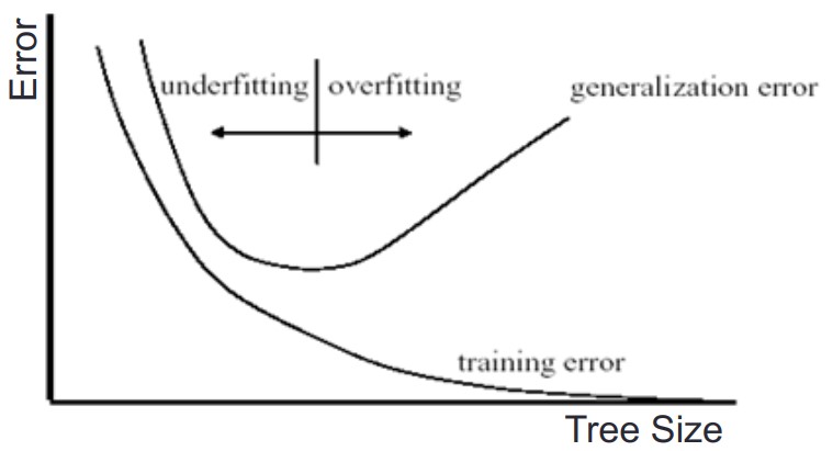
"* **Underfitting & Overfitting** - if we allow Decision Trees to grow until *absolute purity*, we will reach overfitting\n",
" *
Pruning & Regularization Hyperparameters\n",
"---\n",
"* **Underfitting & Overfitting** - if we allow Decision Trees to grow until *absolute purity*, we will reach overfitting\n",
" *  \n",
" * Such model is often called a *nonparametric model*, not because it does not have many parameters (it often has a lot!), but because the number of parameters is not determined prior to learning (the tree keeps on growing).\n",
"* Decision Trees make very few assumptions about the training data (unlike linear models, which assume that the data is linear)."
]
},
{
"cell_type": "markdown",
"metadata": {
"slideshow": {
"slide_type": "subslide"
}
},
"source": [
"* To avoid **overfitting** the training data, we need to restrict the Decision Tree's freedom during training - this is called **regularization**.\n",
"* The methods:\n",
" * **Stop Splitting** - stop growing a tree once a stopping criteria is reached\n",
" * May suffer from the *horizon effect* - such a method will be biased towards trees in which greatest impurity reduction is near the root\n",
" * **Prunning** - grow a full tree, then merge nodes until a stopping criteria is reached or deleting (=prunning) unneccessary nodes if the purity improvement it provides is not *statistically signifacnt*\n",
" * Use Hypothesis Testing - going back to Tutorial 02, standard statistical tests, such as chi-square, $\\chi^2 \\textit{test}$, are used to estimate the probability (*p-value*) that the improvement is purely the result of chance (the *null hypothesis*, $H_0$). If the *p-value* is higher than a given threshold (usually 5%), then the node is considered unneccessary and its children are deleted). The prunning continues until all unnccessary nodes have been pruned."
]
},
{
"cell_type": "markdown",
"metadata": {
"slideshow": {
"slide_type": "subslide"
}
},
"source": [
"* **Common Stopping Criteria** (in practice):\n",
" * *Minimum number of samples* in leaf nodes - **increasing** will regularize the model\n",
" * In Scikit-Learn, set the input parameter `min_samples_leaf`\n",
" * *Minimum samples split* - the minimum number of samples a node must have before it can split, **increasing** will regularize the model\n",
" * In Scikit-Learn, set the input parameter `min_samples_split`\n",
" * *Limit the depth of the tree* - **reducing** the max depth will regularize the model (less chance of overfitting)\n",
" * In Scikit-Learn, set the input parameter `max_depth` (the default is `None` which means unlimited)\n",
" * *Maximum number of leaves* - maximum number of leaf nodes, **reducing** will regularize the model\n",
" * In Scikit-Learn, set the input parameter `max_leaf_nodes`\n",
" * Using the validation accuracy, stop if no significant improvement\n",
" * Also consider `min_weight_fraction_leaf` and `max_features` (more in the Scikit-Learn docs)"
]
},
{
"cell_type": "markdown",
"metadata": {
"slideshow": {
"slide_type": "slide"
}
},
"source": [
"##
\n",
" * Such model is often called a *nonparametric model*, not because it does not have many parameters (it often has a lot!), but because the number of parameters is not determined prior to learning (the tree keeps on growing).\n",
"* Decision Trees make very few assumptions about the training data (unlike linear models, which assume that the data is linear)."
]
},
{
"cell_type": "markdown",
"metadata": {
"slideshow": {
"slide_type": "subslide"
}
},
"source": [
"* To avoid **overfitting** the training data, we need to restrict the Decision Tree's freedom during training - this is called **regularization**.\n",
"* The methods:\n",
" * **Stop Splitting** - stop growing a tree once a stopping criteria is reached\n",
" * May suffer from the *horizon effect* - such a method will be biased towards trees in which greatest impurity reduction is near the root\n",
" * **Prunning** - grow a full tree, then merge nodes until a stopping criteria is reached or deleting (=prunning) unneccessary nodes if the purity improvement it provides is not *statistically signifacnt*\n",
" * Use Hypothesis Testing - going back to Tutorial 02, standard statistical tests, such as chi-square, $\\chi^2 \\textit{test}$, are used to estimate the probability (*p-value*) that the improvement is purely the result of chance (the *null hypothesis*, $H_0$). If the *p-value* is higher than a given threshold (usually 5%), then the node is considered unneccessary and its children are deleted). The prunning continues until all unnccessary nodes have been pruned."
]
},
{
"cell_type": "markdown",
"metadata": {
"slideshow": {
"slide_type": "subslide"
}
},
"source": [
"* **Common Stopping Criteria** (in practice):\n",
" * *Minimum number of samples* in leaf nodes - **increasing** will regularize the model\n",
" * In Scikit-Learn, set the input parameter `min_samples_leaf`\n",
" * *Minimum samples split* - the minimum number of samples a node must have before it can split, **increasing** will regularize the model\n",
" * In Scikit-Learn, set the input parameter `min_samples_split`\n",
" * *Limit the depth of the tree* - **reducing** the max depth will regularize the model (less chance of overfitting)\n",
" * In Scikit-Learn, set the input parameter `max_depth` (the default is `None` which means unlimited)\n",
" * *Maximum number of leaves* - maximum number of leaf nodes, **reducing** will regularize the model\n",
" * In Scikit-Learn, set the input parameter `max_leaf_nodes`\n",
" * Using the validation accuracy, stop if no significant improvement\n",
" * Also consider `min_weight_fraction_leaf` and `max_features` (more in the Scikit-Learn docs)"
]
},
{
"cell_type": "markdown",
"metadata": {
"slideshow": {
"slide_type": "slide"
}
},
"source": [
"##  Example - Titanic Dataset\n",
"---\n",
"The sinking of the RMS Titanic is one of the most infamous shipwrecks in history. On April 15, 1912, during her maiden voyage, the Titanic sank after colliding with an iceberg, killing 1502 out of 2224 passengers and crew. This sensational tragedy shocked the international community and led to better safety regulations for ships.\n",
"\n",
"One of the reasons that the shipwreck led to such loss of life was that there were not enough lifeboats for the passengers and crew. Although there was some element of luck involved in surviving the sinking, some groups of people were more likely to survive than others, such as women, children, and the upper-class.\n",
"\n",
"We will build a decision tree to decide what sorts of people were likely to survive.\n",
"\n",
"To read more about the dataset and the fields - Click Here"
]
},
{
"cell_type": "code",
"execution_count": 2,
"metadata": {
"slideshow": {
"slide_type": "subslide"
}
},
"outputs": [
{
"data": {
"text/html": [
"
Example - Titanic Dataset\n",
"---\n",
"The sinking of the RMS Titanic is one of the most infamous shipwrecks in history. On April 15, 1912, during her maiden voyage, the Titanic sank after colliding with an iceberg, killing 1502 out of 2224 passengers and crew. This sensational tragedy shocked the international community and led to better safety regulations for ships.\n",
"\n",
"One of the reasons that the shipwreck led to such loss of life was that there were not enough lifeboats for the passengers and crew. Although there was some element of luck involved in surviving the sinking, some groups of people were more likely to survive than others, such as women, children, and the upper-class.\n",
"\n",
"We will build a decision tree to decide what sorts of people were likely to survive.\n",
"\n",
"To read more about the dataset and the fields - Click Here"
]
},
{
"cell_type": "code",
"execution_count": 2,
"metadata": {
"slideshow": {
"slide_type": "subslide"
}
},
"outputs": [
{
"data": {
"text/html": [
"\n",
"\n",
"\n",
" \n",
"
\n",
"
"
],
"text/plain": [
" PassengerId Survived Pclass \\\n",
"201 202 0 3 \n",
"333 334 0 3 \n",
"639 640 0 3 \n",
"803 804 1 3 \n",
"871 872 1 1 \n",
"571 572 1 1 \n",
"99 100 0 2 \n",
"783 784 0 3 \n",
"73 74 0 3 \n",
"653 654 1 3 \n",
"\n",
" Name Sex Age SibSp \\\n",
"201 Sage, Mr. Frederick male NaN 8 \n",
"333 Vander Planke, Mr. Leo Edmondus male 16.00 2 \n",
"639 Thorneycroft, Mr. Percival male NaN 1 \n",
"803 Thomas, Master. Assad Alexander male 0.42 0 \n",
"871 Beckwith, Mrs. Richard Leonard (Sallie Monypeny) female 47.00 1 \n",
"571 Appleton, Mrs. Edward Dale (Charlotte Lamson) female 53.00 2 \n",
"99 Kantor, Mr. Sinai male 34.00 1 \n",
"783 Johnston, Mr. Andrew G male NaN 1 \n",
"73 Chronopoulos, Mr. Apostolos male 26.00 1 \n",
"653 O'Leary, Miss. Hanora \"Norah\" female NaN 0 \n",
"\n",
" Parch Ticket Fare Cabin Embarked \n",
"201 2 CA. 2343 69.5500 NaN S \n",
"333 0 345764 18.0000 NaN S \n",
"639 0 376564 16.1000 NaN S \n",
"803 1 2625 8.5167 NaN C \n",
"871 1 11751 52.5542 D35 S \n",
"571 0 11769 51.4792 C101 S \n",
"99 0 244367 26.0000 NaN S \n",
"783 2 W./C. 6607 23.4500 NaN S \n",
"73 0 2680 14.4542 NaN C \n",
"653 0 330919 7.8292 NaN Q "
]
},
"execution_count": 2,
"metadata": {},
"output_type": "execute_result"
}
],
"source": [
"# let's load the titanic dataset and speratre it into train and test set\n",
"dataset = pd.read_csv('./datasets/titanic_dataset.csv')\n",
"# print the number of rows in the data set\n",
"number_of_rows = len(dataset)\n",
"num_train = int(0.8 * number_of_rows)\n",
"# reminder, the data looks like this\n",
"dataset.sample(10)"
]
},
{
"cell_type": "code",
"execution_count": 3,
"metadata": {
"slideshow": {
"slide_type": "skip"
}
},
"outputs": [],
"source": [
"# preprocessing\n",
"original_ds = dataset.copy() # Using 'copy()' allows to clone the dataset, creating a different object with the same values\n",
"dataset['Has_Cabin'] = dataset[\"Cabin\"].apply(lambda x: 0 if type(x) == float else 1)\n",
"# Create new feature FamilySize as a combination of SibSp and Parch\n",
"dataset['FamilySize'] = dataset['SibSp'] + dataset['Parch'] + 1\n",
"# Create new feature IsAlone from FamilySize\n",
"dataset['IsAlone'] = 0\n",
"dataset.loc[dataset['FamilySize'] == 1, 'IsAlone'] = 1\n",
"# Remove all NULLS in the Embarked column\n",
"dataset['Embarked'] = dataset['Embarked'].fillna('S')\n",
"# Remove all NULLS in the Fare column\n",
"dataset['Fare'] = dataset['Fare'].fillna(dataset['Fare'].median())\n",
"\n",
"# Remove all NULLS in the Age column\n",
"age_avg = dataset['Age'].mean()\n",
"age_std = dataset['Age'].std()\n",
"age_null_count = dataset['Age'].isnull().sum()\n",
"age_null_random_list = np.random.randint(age_avg - age_std, age_avg + age_std, size=age_null_count)\n",
"# Next line has been improved to avoid warning\n",
"dataset.loc[np.isnan(dataset['Age']), 'Age'] = age_null_random_list\n",
"dataset['Age'] = dataset['Age'].astype(int)\n",
"\n",
"# Define function to extract titles from passenger names\n",
"def get_title(name):\n",
" title_search = re.search(' ([A-Za-z]+)\\.', name)\n",
" # If the title exists, extract and return it.\n",
" if title_search:\n",
" return title_search.group(1)\n",
" return \"\"\n",
"\n",
"dataset['Title'] = dataset['Name'].apply(get_title)\n",
"\n",
"# Group all non-common titles into one single grouping \"Rare\"\n",
"dataset['Title'] = dataset['Title'].replace(['Lady', 'Countess','Capt', 'Col','Don', 'Dr', 'Major',\n",
" 'Rev', 'Sir', 'Jonkheer', 'Dona'], 'Rare')\n",
"dataset['Title'] = dataset['Title'].replace('Mlle', 'Miss')\n",
"dataset['Title'] = dataset['Title'].replace('Ms', 'Miss')\n",
"dataset['Title'] = dataset['Title'].replace('Mme', 'Mrs')\n",
"\n",
"# mapping\n",
"# Mapping Sex\n",
"dataset['Sex'] = dataset['Sex'].map( {'female': 0, 'male': 1} ).astype(int) \n",
"# Mapping titles\n",
"title_mapping = {\"Mr\": 1, \"Master\": 2, \"Mrs\": 3, \"Miss\": 4, \"Rare\": 5}\n",
"dataset['Title'] = dataset['Title'].map(title_mapping)\n",
"dataset['Title'] = dataset['Title'].fillna(0)\n",
"# Mapping Embarked\n",
"dataset['Embarked'] = dataset['Embarked'].map( {'S': 0, 'C': 1, 'Q': 2} ).astype(int)\n",
"# Mapping Fare\n",
"dataset.loc[ dataset['Fare'] <= 7.91, 'Fare'] = 0\n",
"dataset.loc[(dataset['Fare'] > 7.91) & (dataset['Fare'] <= 14.454), 'Fare'] = 1\n",
"dataset.loc[(dataset['Fare'] > 14.454) & (dataset['Fare'] <= 31), 'Fare'] = 2\n",
"dataset.loc[ dataset['Fare'] > 31, 'Fare'] = 3\n",
"dataset['Fare'] = dataset['Fare'].astype(int)\n",
"\n",
"# Mapping Age\n",
"dataset.loc[ dataset['Age'] <= 16, 'Age'] = 0\n",
"dataset.loc[(dataset['Age'] > 16) & (dataset['Age'] <= 32), 'Age'] = 1\n",
"dataset.loc[(dataset['Age'] > 32) & (dataset['Age'] <= 48), 'Age'] = 2\n",
"dataset.loc[(dataset['Age'] > 48) & (dataset['Age'] <= 64), 'Age'] = 3\n",
"dataset.loc[ dataset['Age'] > 64, 'Age']\n",
"\n",
"# Feature selection: remove variables no longer containing relevant information\n",
"drop_elements = ['PassengerId', 'Name', 'Ticket', 'Cabin', 'SibSp']\n",
"dataset = dataset.drop(drop_elements, axis=1)"
]
},
{
"cell_type": "code",
"execution_count": 4,
"metadata": {
"slideshow": {
"slide_type": "subslide"
}
},
"outputs": [
{
"data": {
"text/html": [
"| \n", " | PassengerId | \n", "Survived | \n", "Pclass | \n", "Name | \n", "Sex | \n", "Age | \n", "SibSp | \n", "Parch | \n", "Ticket | \n", "Fare | \n", "Cabin | \n", "Embarked | \n", "
|---|---|---|---|---|---|---|---|---|---|---|---|---|
| 201 | \n", "202 | \n", "0 | \n", "3 | \n", "Sage, Mr. Frederick | \n", "male | \n", "NaN | \n", "8 | \n", "2 | \n", "CA. 2343 | \n", "69.5500 | \n", "NaN | \n", "S | \n", "
| 333 | \n", "334 | \n", "0 | \n", "3 | \n", "Vander Planke, Mr. Leo Edmondus | \n", "male | \n", "16.00 | \n", "2 | \n", "0 | \n", "345764 | \n", "18.0000 | \n", "NaN | \n", "S | \n", "
| 639 | \n", "640 | \n", "0 | \n", "3 | \n", "Thorneycroft, Mr. Percival | \n", "male | \n", "NaN | \n", "1 | \n", "0 | \n", "376564 | \n", "16.1000 | \n", "NaN | \n", "S | \n", "
| 803 | \n", "804 | \n", "1 | \n", "3 | \n", "Thomas, Master. Assad Alexander | \n", "male | \n", "0.42 | \n", "0 | \n", "1 | \n", "2625 | \n", "8.5167 | \n", "NaN | \n", "C | \n", "
| 871 | \n", "872 | \n", "1 | \n", "1 | \n", "Beckwith, Mrs. Richard Leonard (Sallie Monypeny) | \n", "female | \n", "47.00 | \n", "1 | \n", "1 | \n", "11751 | \n", "52.5542 | \n", "D35 | \n", "S | \n", "
| 571 | \n", "572 | \n", "1 | \n", "1 | \n", "Appleton, Mrs. Edward Dale (Charlotte Lamson) | \n", "female | \n", "53.00 | \n", "2 | \n", "0 | \n", "11769 | \n", "51.4792 | \n", "C101 | \n", "S | \n", "
| 99 | \n", "100 | \n", "0 | \n", "2 | \n", "Kantor, Mr. Sinai | \n", "male | \n", "34.00 | \n", "1 | \n", "0 | \n", "244367 | \n", "26.0000 | \n", "NaN | \n", "S | \n", "
| 783 | \n", "784 | \n", "0 | \n", "3 | \n", "Johnston, Mr. Andrew G | \n", "male | \n", "NaN | \n", "1 | \n", "2 | \n", "W./C. 6607 | \n", "23.4500 | \n", "NaN | \n", "S | \n", "
| 73 | \n", "74 | \n", "0 | \n", "3 | \n", "Chronopoulos, Mr. Apostolos | \n", "male | \n", "26.00 | \n", "1 | \n", "0 | \n", "2680 | \n", "14.4542 | \n", "NaN | \n", "C | \n", "
| 653 | \n", "654 | \n", "1 | \n", "3 | \n", "O'Leary, Miss. Hanora \"Norah\" | \n", "female | \n", "NaN | \n", "0 | \n", "0 | \n", "330919 | \n", "7.8292 | \n", "NaN | \n", "Q | \n", "
\n",
"\n",
"\n",
" \n",
"
\n",
"
"
],
"text/plain": [
" Survived Pclass Sex Age Parch Fare Embarked Has_Cabin FamilySize \\\n",
"359 1 3 0 1 0 0 2 0 1 \n",
"505 0 1 1 1 0 3 1 1 2 \n",
"566 0 3 1 1 0 0 0 0 1 \n",
"878 0 3 1 1 0 0 0 0 1 \n",
"843 0 3 1 2 0 0 1 0 1 \n",
"884 0 3 1 1 0 0 0 0 1 \n",
"685 0 2 1 1 2 3 1 0 4 \n",
"851 0 3 1 74 0 0 0 0 1 \n",
"64 0 1 1 2 0 2 1 0 1 \n",
"373 0 1 1 1 0 3 1 0 1 \n",
"\n",
" IsAlone Title \n",
"359 1 4 \n",
"505 0 1 \n",
"566 1 1 \n",
"878 1 1 \n",
"843 1 1 \n",
"884 1 1 \n",
"685 0 1 \n",
"851 1 1 \n",
"64 1 1 \n",
"373 1 1 "
]
},
"execution_count": 4,
"metadata": {},
"output_type": "execute_result"
}
],
"source": [
"# show a sample of the preprocessed dataset\n",
"dataset.sample(10)"
]
},
{
"cell_type": "code",
"execution_count": 5,
"metadata": {
"slideshow": {
"slide_type": "subslide"
}
},
"outputs": [
{
"name": "stdout",
"output_type": "stream",
"text": [
"total training samples: 712, total test samples: 179\n"
]
}
],
"source": [
"# Take the relevant training data and labels\n",
"x = dataset.drop('Survived', axis=1).values\n",
"y = dataset['Survived'].values # 1 for Survived, 0 for Dead\n",
"# shuffle\n",
"rand_gen = np.random.RandomState(0)\n",
"shuffled_indices = rand_gen.permutation(np.arange(len(x)))\n",
"\n",
"x_train = x[shuffled_indices[:num_train]]\n",
"y_train = y[shuffled_indices[:num_train]]\n",
"x_test = x[shuffled_indices[num_train:]]\n",
"y_test = y[shuffled_indices[num_train:]]\n",
"\n",
"print(\"total training samples: {}, total test samples: {}\".format(num_train, number_of_rows - num_train))"
]
},
{
"cell_type": "code",
"execution_count": 6,
"metadata": {
"slideshow": {
"slide_type": "subslide"
}
},
"outputs": [
{
"data": {
"text/plain": [
"DecisionTreeClassifier(class_weight=None, criterion='gini', max_depth=None,\n",
" max_features=None, max_leaf_nodes=None,\n",
" min_impurity_decrease=0.0, min_impurity_split=None,\n",
" min_samples_leaf=1, min_samples_split=2,\n",
" min_weight_fraction_leaf=0.0, presort=False,\n",
" random_state=None, splitter='best')"
]
},
"execution_count": 6,
"metadata": {},
"output_type": "execute_result"
}
],
"source": [
"# let's build a tree with no limitations\n",
"tree_clf = DecisionTreeClassifier(criterion='gini')\n",
"tree_clf.fit(x_train, y_train)"
]
},
{
"cell_type": "code",
"execution_count": 7,
"metadata": {
"slideshow": {
"slide_type": "subslide"
}
},
"outputs": [
{
"name": "stdout",
"output_type": "stream",
"text": [
"accuracy: 75.419 %\n"
]
}
],
"source": [
"# let's check the accuracy on the test set\n",
"y_pred = tree_clf.predict(x_test)\n",
"accuracy = np.sum(y_pred == y_test) / len(y_test)\n",
"print(\"accuracy: {:.3f} %\".format(accuracy * 100))"
]
},
{
"cell_type": "code",
"execution_count": 8,
"metadata": {
"slideshow": {
"slide_type": "subslide"
}
},
"outputs": [
{
"name": "stdout",
"output_type": "stream",
"text": [
"accuracy: 83.799 %\n"
]
}
],
"source": [
"# let's add regularization\n",
"tree_clf = DecisionTreeClassifier(criterion='gini', max_depth=3)\n",
"tree_clf.fit(x_train, y_train)\n",
"# let's check the accuracy on the test set\n",
"y_pred = tree_clf.predict(x_test)\n",
"accuracy = np.sum(y_pred == y_test) / len(y_test)\n",
"print(\"accuracy: {:.3f} %\".format(accuracy * 100))"
]
},
{
"cell_type": "code",
"execution_count": 9,
"metadata": {
"slideshow": {
"slide_type": "subslide"
}
},
"outputs": [
{
"name": "stdout",
"output_type": "stream",
"text": [
"passenger 0 chances of survival: 89.318 %\n"
]
}
],
"source": [
"# predicting probabilities\n",
"# for the first passenger in the test set, the probability of survival:\n",
"prob = tree_clf.predict_proba([x_train[0]])\n",
"print(\"passenger 0 chances of survival: {:.3f} %\".format(prob[0][0] * 100))"
]
},
{
"cell_type": "code",
"execution_count": null,
"metadata": {
"slideshow": {
"slide_type": "subslide"
}
},
"outputs": [],
"source": [
"# generate an image graph\n",
"from sklearn.tree import export_graphviz\n",
"export_graphviz(tree_clf, out_file=\"./titanic_tree.dot\", feature_names=dataset.columns.values[1:].tolist(), \n",
" class_names=['Dead', 'Survived'], rounded=True, filled=True)\n",
"# open the file with your favourite text editor and copy-pase it into http://www.webgraphviz.com/"
]
},
{
"cell_type": "markdown",
"metadata": {
"slideshow": {
"slide_type": "subslide"
}
},
"source": [
"| \n", " | Survived | \n", "Pclass | \n", "Sex | \n", "Age | \n", "Parch | \n", "Fare | \n", "Embarked | \n", "Has_Cabin | \n", "FamilySize | \n", "IsAlone | \n", "Title | \n", "
|---|---|---|---|---|---|---|---|---|---|---|---|
| 359 | \n", "1 | \n", "3 | \n", "0 | \n", "1 | \n", "0 | \n", "0 | \n", "2 | \n", "0 | \n", "1 | \n", "1 | \n", "4 | \n", "
| 505 | \n", "0 | \n", "1 | \n", "1 | \n", "1 | \n", "0 | \n", "3 | \n", "1 | \n", "1 | \n", "2 | \n", "0 | \n", "1 | \n", "
| 566 | \n", "0 | \n", "3 | \n", "1 | \n", "1 | \n", "0 | \n", "0 | \n", "0 | \n", "0 | \n", "1 | \n", "1 | \n", "1 | \n", "
| 878 | \n", "0 | \n", "3 | \n", "1 | \n", "1 | \n", "0 | \n", "0 | \n", "0 | \n", "0 | \n", "1 | \n", "1 | \n", "1 | \n", "
| 843 | \n", "0 | \n", "3 | \n", "1 | \n", "2 | \n", "0 | \n", "0 | \n", "1 | \n", "0 | \n", "1 | \n", "1 | \n", "1 | \n", "
| 884 | \n", "0 | \n", "3 | \n", "1 | \n", "1 | \n", "0 | \n", "0 | \n", "0 | \n", "0 | \n", "1 | \n", "1 | \n", "1 | \n", "
| 685 | \n", "0 | \n", "2 | \n", "1 | \n", "1 | \n", "2 | \n", "3 | \n", "1 | \n", "0 | \n", "4 | \n", "0 | \n", "1 | \n", "
| 851 | \n", "0 | \n", "3 | \n", "1 | \n", "74 | \n", "0 | \n", "0 | \n", "0 | \n", "0 | \n", "1 | \n", "1 | \n", "1 | \n", "
| 64 | \n", "0 | \n", "1 | \n", "1 | \n", "2 | \n", "0 | \n", "2 | \n", "1 | \n", "0 | \n", "1 | \n", "1 | \n", "1 | \n", "
| 373 | \n", "0 | \n", "1 | \n", "1 | \n", "1 | \n", "0 | \n", "3 | \n", "1 | \n", "0 | \n", "1 | \n", "1 | \n", "1 | \n", "
 "
]
},
{
"cell_type": "markdown",
"metadata": {
"slideshow": {
"slide_type": "slide"
}
},
"source": [
"##
"
]
},
{
"cell_type": "markdown",
"metadata": {
"slideshow": {
"slide_type": "slide"
}
},
"source": [
"##  Random Forest\n",
"---\n",
"* Random forests (or random decision forests) are an **ensemble learning** method for classification, regression and other tasks.\n",
"* They operate by constructing a multitude of decision trees at training time and outputting the class that is the mode of the classes (classification) or mean prediction (regression) of the individual trees.\n",
" * We will talk on ensemble learning later in the course.\n",
"* Random decision forests try tend to decision trees' habit of overfitting to their training set."
]
},
{
"cell_type": "markdown",
"metadata": {
"slideshow": {
"slide_type": "subslide"
}
},
"source": [
"
Random Forest\n",
"---\n",
"* Random forests (or random decision forests) are an **ensemble learning** method for classification, regression and other tasks.\n",
"* They operate by constructing a multitude of decision trees at training time and outputting the class that is the mode of the classes (classification) or mean prediction (regression) of the individual trees.\n",
" * We will talk on ensemble learning later in the course.\n",
"* Random decision forests try tend to decision trees' habit of overfitting to their training set."
]
},
{
"cell_type": "markdown",
"metadata": {
"slideshow": {
"slide_type": "subslide"
}
},
"source": [
" \n",
"\n",
"* Image Source"
]
},
{
"cell_type": "markdown",
"metadata": {
"slideshow": {
"slide_type": "subslide"
}
},
"source": [
"#### Random Forest Algorithm\n",
"---\n",
"* The training algorithm for random forests applies **bootstrap aggregating, or bagging** (tutorial 11), to tree learners.\n",
"* Given a training set $X = x_1, ..., x_n$ with targets $Y = y_1, ..., y_n$, bagging repeatedly ($B$ times) selects a **random sample with replacement** of the training set and fits trees to these samples:\n",
" * For $b = 1,...,B$:\n",
" * Sample, with replacement, $n$ training examples from $X, Y$; call these $X_b, Y_b$.\n",
" * Train a classification or regression tree $f_b$ on $X_b, Y_b$.\n",
" * After training, predictions for unseen samples $x'$ can be made by averaging the predictions from all the individual regression trees on $x'$: $$ \\hat{f} = \\frac{1}{B} \\sum_{i=1}^B f_b(x') $$\n",
" * Or by taking the **majority vote** in the case of *classification* trees."
]
},
{
"cell_type": "code",
"execution_count": 29,
"metadata": {
"slideshow": {
"slide_type": "subslide"
}
},
"outputs": [
{
"name": "stdout",
"output_type": "stream",
"text": [
"accuracy: 84.916 %\n"
]
}
],
"source": [
"from sklearn.ensemble import RandomForestClassifier\n",
"random_state= 42\n",
"rnd_clf = RandomForestClassifier(random_state=random_state, n_estimators=50, max_depth=3)\n",
"rnd_clf.fit(x_train, y_train)\n",
"# let's check the accuracy on the test set\n",
"y_pred = rnd_clf.predict(x_test)\n",
"accuracy = np.sum(y_pred == y_test) / len(y_test)\n",
"print(\"accuracy: {:.3f} %\".format(accuracy * 100))"
]
},
{
"cell_type": "markdown",
"metadata": {
"slideshow": {
"slide_type": "subslide"
}
},
"source": [
"* This bootstrapping procedure leads to better model performance because it decreases the *variance* of the model, without increasing the *bias*. \n",
"* This means that while the predictions of a single tree are highly sensitive to noise in its training set, the average of many trees is not, as long as the trees are not correlated. \n",
"* Simply training many trees on a single training set would give strongly correlated trees (or even the same tree many times, if the training algorithm is deterministic).\n",
" * Bootstrap sampling is a way of de-correlating the trees by showing them different training sets."
]
},
{
"cell_type": "markdown",
"metadata": {
"slideshow": {
"slide_type": "slide"
}
},
"source": [
"###
\n",
"\n",
"* Image Source"
]
},
{
"cell_type": "markdown",
"metadata": {
"slideshow": {
"slide_type": "subslide"
}
},
"source": [
"#### Random Forest Algorithm\n",
"---\n",
"* The training algorithm for random forests applies **bootstrap aggregating, or bagging** (tutorial 11), to tree learners.\n",
"* Given a training set $X = x_1, ..., x_n$ with targets $Y = y_1, ..., y_n$, bagging repeatedly ($B$ times) selects a **random sample with replacement** of the training set and fits trees to these samples:\n",
" * For $b = 1,...,B$:\n",
" * Sample, with replacement, $n$ training examples from $X, Y$; call these $X_b, Y_b$.\n",
" * Train a classification or regression tree $f_b$ on $X_b, Y_b$.\n",
" * After training, predictions for unseen samples $x'$ can be made by averaging the predictions from all the individual regression trees on $x'$: $$ \\hat{f} = \\frac{1}{B} \\sum_{i=1}^B f_b(x') $$\n",
" * Or by taking the **majority vote** in the case of *classification* trees."
]
},
{
"cell_type": "code",
"execution_count": 29,
"metadata": {
"slideshow": {
"slide_type": "subslide"
}
},
"outputs": [
{
"name": "stdout",
"output_type": "stream",
"text": [
"accuracy: 84.916 %\n"
]
}
],
"source": [
"from sklearn.ensemble import RandomForestClassifier\n",
"random_state= 42\n",
"rnd_clf = RandomForestClassifier(random_state=random_state, n_estimators=50, max_depth=3)\n",
"rnd_clf.fit(x_train, y_train)\n",
"# let's check the accuracy on the test set\n",
"y_pred = rnd_clf.predict(x_test)\n",
"accuracy = np.sum(y_pred == y_test) / len(y_test)\n",
"print(\"accuracy: {:.3f} %\".format(accuracy * 100))"
]
},
{
"cell_type": "markdown",
"metadata": {
"slideshow": {
"slide_type": "subslide"
}
},
"source": [
"* This bootstrapping procedure leads to better model performance because it decreases the *variance* of the model, without increasing the *bias*. \n",
"* This means that while the predictions of a single tree are highly sensitive to noise in its training set, the average of many trees is not, as long as the trees are not correlated. \n",
"* Simply training many trees on a single training set would give strongly correlated trees (or even the same tree many times, if the training algorithm is deterministic).\n",
" * Bootstrap sampling is a way of de-correlating the trees by showing them different training sets."
]
},
{
"cell_type": "markdown",
"metadata": {
"slideshow": {
"slide_type": "slide"
}
},
"source": [
"###  Recommended Videos\n",
"---\n",
"####
Recommended Videos\n",
"---\n",
"####  Warning!\n",
"* These videos do not replace the lectures and tutorials.\n",
"* Please use these to get a better understanding of the material, and not as an alternative to the written material.\n",
"\n",
"#### Video By Subject\n",
"\n",
"* Decision Trees - Machine Learning Lecture 29 \"Decision Trees / Regression Trees\" -Cornell CS4780\n",
"* Decision Trees Example with Gini - StatQuest: Decision Trees\n",
"* Information Gain, Mutual Information - Decision Tree 4: Information Gain\n",
"* Random Forests - Random Forest - Fun and Easy Machine Learning\n",
" * Random Forests / Bagging - Machine Learning Lecture 31 \"Random Forests / Bagging\" -Cornell CS4780"
]
},
{
"cell_type": "markdown",
"metadata": {
"slideshow": {
"slide_type": "skip"
}
},
"source": [
"##
Warning!\n",
"* These videos do not replace the lectures and tutorials.\n",
"* Please use these to get a better understanding of the material, and not as an alternative to the written material.\n",
"\n",
"#### Video By Subject\n",
"\n",
"* Decision Trees - Machine Learning Lecture 29 \"Decision Trees / Regression Trees\" -Cornell CS4780\n",
"* Decision Trees Example with Gini - StatQuest: Decision Trees\n",
"* Information Gain, Mutual Information - Decision Tree 4: Information Gain\n",
"* Random Forests - Random Forest - Fun and Easy Machine Learning\n",
" * Random Forests / Bagging - Machine Learning Lecture 31 \"Random Forests / Bagging\" -Cornell CS4780"
]
},
{
"cell_type": "markdown",
"metadata": {
"slideshow": {
"slide_type": "skip"
}
},
"source": [
"##  Credits\n",
"---\n",
"* Based upon *Pattern Classification*, chapter 8\n",
"* Information Gain and Mutual Information for Machine Learning\n",
"* Icons from Icon8.com - https://icons8.com\n",
"* Datasets from Kaggle - https://www.kaggle.com/\n",
"* Examples and code snippets were taken from \"Hands-On Machine Learning with Scikit-Learn and TensorFlow\""
]
}
],
"metadata": {
"kernelspec": {
"display_name": "Python 3",
"language": "python",
"name": "python3"
},
"language_info": {
"codemirror_mode": {
"name": "ipython",
"version": 3
},
"file_extension": ".py",
"mimetype": "text/x-python",
"name": "python",
"nbconvert_exporter": "python",
"pygments_lexer": "ipython3",
"version": "3.6.9"
}
},
"nbformat": 4,
"nbformat_minor": 2
}
Credits\n",
"---\n",
"* Based upon *Pattern Classification*, chapter 8\n",
"* Information Gain and Mutual Information for Machine Learning\n",
"* Icons from Icon8.com - https://icons8.com\n",
"* Datasets from Kaggle - https://www.kaggle.com/\n",
"* Examples and code snippets were taken from \"Hands-On Machine Learning with Scikit-Learn and TensorFlow\""
]
}
],
"metadata": {
"kernelspec": {
"display_name": "Python 3",
"language": "python",
"name": "python3"
},
"language_info": {
"codemirror_mode": {
"name": "ipython",
"version": 3
},
"file_extension": ".py",
"mimetype": "text/x-python",
"name": "python",
"nbconvert_exporter": "python",
"pygments_lexer": "ipython3",
"version": "3.6.9"
}
},
"nbformat": 4,
"nbformat_minor": 2
}