---
title: "Project Report Title"
author: "First Last"
date: last-modified
format:
html:
theme: cosmo # also try flatly or lumen
toc: true
toc-depth: 3
toc-location: left
number-sections: true
code-fold: false
code-tools: true
fig-cap-location: bottom
df-print: kable
embed-resources: true
bibliography: bibtex.bib
---
## Quarto Overview
Quarto combines markdown (an easy to write plain text format) with embedded
R code chunks. When compiling Quarto documents, the code components can be
evaluated so that both the code and its output can be included in the final
document. This makes analysis reports highly reproducible by allowing to automatically
regenerate them when the underlying R code or data changes. Quarto
documents (`.qmd` files) can be rendered to various formats including HTML and
PDF. The R code in an `.qmd` document is processed by `knitr`, while the
resulting `.md` file is rendered by `pandoc` to the final output formats
(_e.g._ HTML or PDF). Historically, Quarto is an extension of the older
`Sweave/Latex` environment. Rendering of mathematical expressions and reference
management is also supported by Quarto using embedded Latex syntax and
Bibtex, respectively. A new and related publishing environemt is [Quarto](https://quarto.org/docs/tools/neovim.html) (not covered here).
## Quick Start
### Install Quarto
To work with this tutorial, the `rmarkdown` package needs to be installed on a system.
```{r install_rmarkdown}
#| eval: false
install.packages("quarto")
```
### Initialize a new Quarto (`qmd`) script
To minimize typing, it can be helful to start with a Quarto template ([here](https://girke.bioinformatics.ucr.edu/GEN242/tutorials/quarto/quarto_index.html#metadata-section)) and
then modify it as needed. Note the file name of a Quarto scirpt needs to
have the extension `.qmd`. The template files for the following exercises are available
here:
+ Quarto sample script: [`sample.qmd`](https://raw.githubusercontent.com/tgirke/GEN242/refs/heads/main/tutorials/quarto/sample.qmd)
+ Bibtex file for handling citations and reference section: [`bibtex.bib`](https://raw.githubusercontent.com/tgirke/GEN242/refs/heads/main/tutorials/quarto/bibtex.bib)
Users want to download these files, open the `sample.qmd` file with their preferred R IDE
(_e.g._ RStudio, Nvim-R-Tmux or emacs), initilize an R session and then direct their R session to
the location of these two files.
### Metadata section
The metadata section (YAML header) in an Quarto script defines how it will be processed and
rendered. The metadata section also includes both title, author, and date information as well as
options for customizing the output format. For instance, PDF and HTML output can be defined
with `pdf_document` and `html_document`, respectively.
```
---
title: "Project Report Title"
author: "First Last"
date: last-modified
format:
html:
theme: cosmo # also try flatly or lumen
toc: true
toc-depth: 3
toc-location: left
number-sections: true
code-fold: false
code-tools: true
fig-cap-location: bottom
df-print: kable
embed-resources: true
bibliography: bibtex.bib
---
```
### Render `qmd` script
A Quarto script can be evaluated and rendered with the following `quarto_render` command or by pressing the `knit` button in RStudio.
The `output_format` argument defines the format of the output.
```{r render_rmarkdown, eval=FALSE, message=FALSE}
quarto::quarto_render("sample.qmd") # default format from YAML
quarto::quarto_render("sample.qmd", output_format="pdf")
```
The following shows how to render a `qmd` file from the command-line. To render to PDF format, use the argument setting: `output_format="pdf_document"` or `--to pdf` from R or command-line, respectively.
```{sh render_commandline}
#| eval: false
#| message: false
quarto render sample.qmd
quarto render sample.qmd --to pdf
```
### R code chunks
R Code Chunks can be embedded in a Quarto script by using three backticks
at the beginning of a new line along with arguments in the following lines starting
with `#|` that control the behavior of the code. The following lines contain the
plain R code. A code chunk is terminated by a new line starting with three backticks.
````{verbatim}
```{r code_chunk_name}
#| eval: false
x <- 1:10
```
````
The most important chunk options are:
+ `eval: true/false` — execute the chunk
+ `echo: true/false` — show the source code in the output
+ `warning: false` — suppress warnings
+ `message: false` — suppress messages
+ `cache: true` — cache results to speed up re-rendering
+ `fig-height: 4` — figure height in inches
+ `fig-width: 6` — figure width in inches
+ `fig-cap: "..."` — figure caption
+ `label: fig-name` — chunk label for cross-referencing (must start with `fig-` for figures)
For more details on chunk caching see the
[knitr cache documentation](https://bookdown.org/yihui/rmarkdown-cookbook/cache.html).
### Learning Markdown
Quarto uses standard Markdown for prose. The syntax is minimal and easy to learn:
+ [Quarto Markdown Basics](https://quarto.org/docs/authoring/markdown-basics.html)
+ [Markdown Intro on GitHub](https://guides.github.com/features/mastering-markdown/)
+ [Markdown Cheat Sheet](https://github.com/adam-p/markdown-here/wiki/Markdown-Cheatsheet)
+ [Quarto cheatsheet](https://rstudio.github.io/cheatsheets/quarto.pdf)
### Tables
There are several ways to render tables. First, they can be printed within the R code chunks. Second,
much nicer formatted tables can be generated with the functions `kable`, `kableExtra`, `pander` or `xtable`. The following
example uses `kable` from the `knitr` package.
### With `knitr::kable`
```{r kable}
library(knitr)
kable(iris[1:12,])
```
A much more elegant and powerful solution is to create fully interactive tables with the [`DT` package](https://rstudio.github.io/DT/).
This JavaScirpt based environment provides a wrapper to the `DataTables` library using jQuery. The resulting tables can be sorted, queried and resized by the
user. Note, Quarto source files containing JavaScript components can only be rendered into HTML and not PDF.
### With `DT::datatable`
```{r dt}
library(DT)
datatable(iris)
```
### Figures
Plots generated by the R code chunks in a Quarto document can be automatically
inserted in the output file. The size of the figure can be controlled with the `fig.height`
and `fig.width` arguments.
```{r some_jitter_plot}
#| eval: true
library(ggplot2)
dsmall <- diamonds[sample(nrow(diamonds), 1000), ]
ggplot(dsmall, aes(color, price/carat)) + geom_jitter(alpha = I(1 / 2), aes(color=color))
```
Sometimes it can be useful to explicitly write an image to a file and then insert that
image into the final document by referencing its file name in the R Markdown source. For
instance, this can be useful for time consuming analyses. The following code will generate a
file named `myplot.png`. To insert the file in the final document, one can use standard
Markdown or HTML syntax, _e.g._: `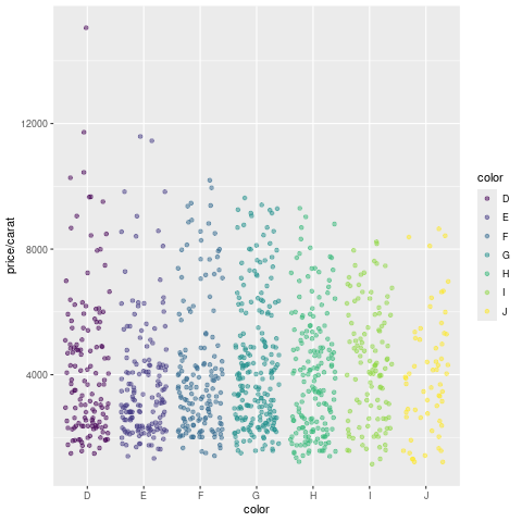 `.
```{r some_custom_inserted_plot}
#| eval: true
#| warning: false
#| message: false
#| results: hide
png("myplot.png")
ggplot(dsmall, aes(color, price/carat)) + geom_jitter(alpha = I(1 / 2), aes(color=color))
dev.off()
```
Quarto has a native cross-referencing system. This works as follows: give a chunk a label starting with `fig-`
and add a caption; then reference it anywhere in the document with `@fig-label`, which
renders as a numbered hyperlink, here @fig-jitter. This name-based referencing scheme
applies to tables (`tbl-` prefix) and sections (`sec-` prefix, requires `number-sections: true`).
Before this extremely useful feature was only available in LaTeX (missing in
R Markdown). Also note: for large documents, like PhD theses, where referencing
of figures and tables across documents is important, this feature is best supported in
[Quarto Books](https://quarto.org/docs/books/). In this context it is also useful to know
that Quarto documents can be converted to `tex` (LaTeX) files.
````{verbatim}
```{r}
#| label: fig-jitter # Note: when label is used, omit name in header line!
#| fig-cap: "Diamond price by color."
#| fig-height: 4
ggplot(dsmall, aes(color, price/carat)) +
geom_jitter(alpha = 0.5, aes(color = color))
```
````
```{r}
#| label: fig-jitter
#| fig-cap: "Diamond price by color."
#| fig-height: 4
ggplot(dsmall, aes(color, price/carat)) +
geom_jitter(alpha = 0.5, aes(color = color))
```
### Custom functions
Custom functions can be kept in a separate R file (here [`custom_Fct.R`](https://raw.githubusercontent.com/tgirke/GEN242/main/content/en/tutorials/rmarkdown/custom_Fct.R)) and then imported
with the `source()` command. In the following example, the `custom_Fct.R` file is located on GitHub.
```{r import_custom_fct}
#| eval: true
source("https://raw.githubusercontent.com/tgirke/GEN242/refs/heads/main/tutorials/quarto/custom_Fct.R")
```
Now the imported function (here `myMAcomp`) can be used.
```{r use_custom_fct}
#| eval: true
myMA <- matrix(rnorm(100000), 10000, 10, dimnames=list(1:10000, paste("C", 1:10, sep="")))
resultDF <- myMAcomp(myMA=myMA, group=c(1,1,1,2,2,2,3,3,4,4), myfct=mean)
kable(resultDF[1:12,])
```
### Inline R code
To evaluate R code inline, one can enclose an R expression with a single back-tick
followed by `r` and then the actual expression. For instance, the back-ticked version
of 'r 1 + 1' evaluates to `r 1 + 1` and 'r pi' evaluates to `r pi`.
### Mathematical equations
To render mathematical equations, one can use standard Latex syntax. When expressions are
enclosed with single `$` signs then they will be shown inline, while
enclosing them with double `$$` signs will show them in display mode. For instance, the following
Latex syntax `d(X,Y) = \sqrt[]{ \sum_{i=1}^{n}{(x_{i}-y_{i})^2} }` renders in display mode as follows:
$$d(X,Y) = \sqrt[]{ \sum_{i=1}^{n}{(x_{i}-y_{i})^2} }$$
To learn LaTeX syntax for mathematical equations, one can consult various online manuals, such as
this [Wikibooks tutorial](https://en.wikibooks.org/wiki/LaTeX/Mathematics), or use an online
equation rendering and checking tool, such as this [one](https://arachnoid.com/latex/).
### Citations and bibliographies
Citations and bibliographies can be autogenerated in Quarto in a similar
way as in Latex/Bibtex. Reference collections should be stored in a separate
file in Bibtex or other supported formats. To cite a publication in a Quarto
script, one uses the syntax `[@]` where `` needs to be replaced with a
reference identifier present in the Bibtex database listed in the metadata section
of the Quarto script (_e.g._ `bibtex.bib`). For instance, to cite Lawrence et al.
(2013), one uses its reference identifier (_e.g._ `Lawrence2013-kt`) as `` [@Lawrence2013-kt].
This will place the citation inline in the text and add the corresponding
reference to a reference list at the end of the output document. For the latter a
special section called `References` needs to be specified at the end of the R Markdown script.
To fine control the formatting of citations and reference lists, users want to consult this
[R Markdown page](http://rmarkdown.rstudio.com/authoring_bibliographies_and_citations.html).
Also, for general reference management and obtaining references in Bibtex format [Paperpile](https://paperpile.com/features)
can be very helpful.
### Viewing Quarto reports on HPCC cluster
Quarto reports located on UCR's HPCC Cluster can be viewed locally in a web browser (without moving
the source HTML) by creating a symbolic link from a user's `.html` directory. This way any updates to
the report will show up immediately without creating another copy of the HTML file. For instance, if user
`ttest` has generated an Quarto report under `~/bigdata/today/rmarkdown/sample.html`, then the
symbolic link can be created as follows:
```{r rmarkdown_symbolic_link}
#| eval: false
cd ~/.html
ln -s ~/bigdata/today/rmarkdown/sample.html sample.html
```
After this one can view the report in a web browser using this URL [https://cluster.hpcc.ucr.edu/~ttest/rmarkdown/sample.html](https://cluster.hpcc.ucr.edu/~ttest/rmarkdown/sample.html).
If necessary access to the URL can be restricted with a password following the instructions [here](http://hpcc.ucr.edu/manuals_linux-cluster_sharing.html#sharing-files-on-the-web).
### Viewing Quarto report on GitHub
To host and view static HTML files on GitHub, follow the instructions [here](https://girke.bioinformatics.ucr.edu/GEN242/tutorials/github/github.html#viewing-static-html-files-on-github). Note, this works
only with public GitHub repos.
## Session Info
```{r sessionInfo}
sessionInfo()
```
## References
`.
```{r some_custom_inserted_plot}
#| eval: true
#| warning: false
#| message: false
#| results: hide
png("myplot.png")
ggplot(dsmall, aes(color, price/carat)) + geom_jitter(alpha = I(1 / 2), aes(color=color))
dev.off()
```
Quarto has a native cross-referencing system. This works as follows: give a chunk a label starting with `fig-`
and add a caption; then reference it anywhere in the document with `@fig-label`, which
renders as a numbered hyperlink, here @fig-jitter. This name-based referencing scheme
applies to tables (`tbl-` prefix) and sections (`sec-` prefix, requires `number-sections: true`).
Before this extremely useful feature was only available in LaTeX (missing in
R Markdown). Also note: for large documents, like PhD theses, where referencing
of figures and tables across documents is important, this feature is best supported in
[Quarto Books](https://quarto.org/docs/books/). In this context it is also useful to know
that Quarto documents can be converted to `tex` (LaTeX) files.
````{verbatim}
```{r}
#| label: fig-jitter # Note: when label is used, omit name in header line!
#| fig-cap: "Diamond price by color."
#| fig-height: 4
ggplot(dsmall, aes(color, price/carat)) +
geom_jitter(alpha = 0.5, aes(color = color))
```
````
```{r}
#| label: fig-jitter
#| fig-cap: "Diamond price by color."
#| fig-height: 4
ggplot(dsmall, aes(color, price/carat)) +
geom_jitter(alpha = 0.5, aes(color = color))
```
### Custom functions
Custom functions can be kept in a separate R file (here [`custom_Fct.R`](https://raw.githubusercontent.com/tgirke/GEN242/main/content/en/tutorials/rmarkdown/custom_Fct.R)) and then imported
with the `source()` command. In the following example, the `custom_Fct.R` file is located on GitHub.
```{r import_custom_fct}
#| eval: true
source("https://raw.githubusercontent.com/tgirke/GEN242/refs/heads/main/tutorials/quarto/custom_Fct.R")
```
Now the imported function (here `myMAcomp`) can be used.
```{r use_custom_fct}
#| eval: true
myMA <- matrix(rnorm(100000), 10000, 10, dimnames=list(1:10000, paste("C", 1:10, sep="")))
resultDF <- myMAcomp(myMA=myMA, group=c(1,1,1,2,2,2,3,3,4,4), myfct=mean)
kable(resultDF[1:12,])
```
### Inline R code
To evaluate R code inline, one can enclose an R expression with a single back-tick
followed by `r` and then the actual expression. For instance, the back-ticked version
of 'r 1 + 1' evaluates to `r 1 + 1` and 'r pi' evaluates to `r pi`.
### Mathematical equations
To render mathematical equations, one can use standard Latex syntax. When expressions are
enclosed with single `$` signs then they will be shown inline, while
enclosing them with double `$$` signs will show them in display mode. For instance, the following
Latex syntax `d(X,Y) = \sqrt[]{ \sum_{i=1}^{n}{(x_{i}-y_{i})^2} }` renders in display mode as follows:
$$d(X,Y) = \sqrt[]{ \sum_{i=1}^{n}{(x_{i}-y_{i})^2} }$$
To learn LaTeX syntax for mathematical equations, one can consult various online manuals, such as
this [Wikibooks tutorial](https://en.wikibooks.org/wiki/LaTeX/Mathematics), or use an online
equation rendering and checking tool, such as this [one](https://arachnoid.com/latex/).
### Citations and bibliographies
Citations and bibliographies can be autogenerated in Quarto in a similar
way as in Latex/Bibtex. Reference collections should be stored in a separate
file in Bibtex or other supported formats. To cite a publication in a Quarto
script, one uses the syntax `[@]` where `` needs to be replaced with a
reference identifier present in the Bibtex database listed in the metadata section
of the Quarto script (_e.g._ `bibtex.bib`). For instance, to cite Lawrence et al.
(2013), one uses its reference identifier (_e.g._ `Lawrence2013-kt`) as `` [@Lawrence2013-kt].
This will place the citation inline in the text and add the corresponding
reference to a reference list at the end of the output document. For the latter a
special section called `References` needs to be specified at the end of the R Markdown script.
To fine control the formatting of citations and reference lists, users want to consult this
[R Markdown page](http://rmarkdown.rstudio.com/authoring_bibliographies_and_citations.html).
Also, for general reference management and obtaining references in Bibtex format [Paperpile](https://paperpile.com/features)
can be very helpful.
### Viewing Quarto reports on HPCC cluster
Quarto reports located on UCR's HPCC Cluster can be viewed locally in a web browser (without moving
the source HTML) by creating a symbolic link from a user's `.html` directory. This way any updates to
the report will show up immediately without creating another copy of the HTML file. For instance, if user
`ttest` has generated an Quarto report under `~/bigdata/today/rmarkdown/sample.html`, then the
symbolic link can be created as follows:
```{r rmarkdown_symbolic_link}
#| eval: false
cd ~/.html
ln -s ~/bigdata/today/rmarkdown/sample.html sample.html
```
After this one can view the report in a web browser using this URL [https://cluster.hpcc.ucr.edu/~ttest/rmarkdown/sample.html](https://cluster.hpcc.ucr.edu/~ttest/rmarkdown/sample.html).
If necessary access to the URL can be restricted with a password following the instructions [here](http://hpcc.ucr.edu/manuals_linux-cluster_sharing.html#sharing-files-on-the-web).
### Viewing Quarto report on GitHub
To host and view static HTML files on GitHub, follow the instructions [here](https://girke.bioinformatics.ucr.edu/GEN242/tutorials/github/github.html#viewing-static-html-files-on-github). Note, this works
only with public GitHub repos.
## Session Info
```{r sessionInfo}
sessionInfo()
```
## References