``'.
```{r comment_lines, eval=TRUE}
readLines(targetspath)[1:4]
```
The function _`readComp`_ imports the comparison information and stores it in a _`list`_. Alternatively, _`readComp`_ can obtain the comparison information from the corresponding _`SYSargs`_ object (see below).
Note, these header lines are optional. They are mainly useful for controlling comparative analyses according to certain biological expectations, such as identifying differentially expressed genes in RNA-Seq experiments based on simple pair-wise comparisons.
```{r targetscomp, eval=TRUE}
readComp(file=targetspath, format="vector", delim="-")
```
[Back to Table of Contents]()
## Structure of _`param`_ file and _`SYSargs`_ container
The _`param`_ file defines the parameters of a chosen command-line software. The following shows the format of a sample _`param`_ file provided by this package.
```{r param_structure, eval=TRUE}
parampath <- system.file("extdata", "tophat.param", package="systemPipeR")
read.delim(parampath, comment.char = "#")
```
The _`systemArgs`_ function imports the definitions of both the _`param`_ file and the _`targets`_ file, and stores all relevant information in a _`SYSargs`_ S4 class object. To run the pipeline without command-line software, one can assign _`NULL`_ to _`sysma`_ instead of a _`param`_ file. In addition, one can start the _`systemPipeR`_ workflow with pre-generated BAM files by providing a targets file where the _`FileName`_ column gives the paths to the BAM files and _`sysma`_ is assigned _`NULL`_.
```{r param_import, eval=TRUE}
args <- suppressWarnings(systemArgs(sysma=parampath, mytargets=targetspath))
args
```
Several accessor functions are available that are named after the slot names of the _`SYSargs`_ object.
```{r sysarg_access, eval=TRUE}
names(args)
modules(args)
cores(args)
outpaths(args)[1]
sysargs(args)[1]
```
The content of the _`param`_ file can also be returned as JSON object as follows (requires _`rjson`_ package).
```{r sysarg_json, eval=TRUE}
systemArgs(sysma=parampath, mytargets=targetspath, type="json")
```
[Back to Table of Contents]()
# Workflow overview
## Define environment settings and samples
Load packages and generate workflow environment (here for RNA-Seq)
```{r load_package, eval=FALSE}
library(systemPipeR)
library(systemPipeRdata)
genWorkenvir(workflow="rnaseq")
setwd("rnaseq")
```
Construct _`SYSargs`_ object from _`param`_ and _`targets`_ files.
```{r construct_sysargs, eval=FALSE}
args <- systemArgs(sysma="param/trim.param", mytargets="targets.txt")
```
[Back to Table of Contents]()
## Read Preprocessing
The function _`preprocessReads`_ allows to apply predefined or custom
read preprocessing functions to all FASTQ files referenced in a
_`SYSargs`_ container, such as quality filtering or adaptor trimming
routines. The paths to the resulting output FASTQ files are stored in the
_`outpaths`_ slot of the _`SYSargs`_ object. Internally,
_`preprocessReads`_ uses the _`FastqStreamer`_ function from
the _`ShortRead`_ package to stream through large FASTQ files in a
memory-efficient manner. The following example performs adaptor trimming with
the _`trimLRPatterns`_ function from the _`Biostrings`_ package.
After the trimming step a new targets file is generated (here
_`targets_trim.txt`_) containing the paths to the trimmed FASTQ files.
The new targets file can be used for the next workflow step with an updated
_`SYSargs`_ instance, \textit{e.g.} running the NGS alignments using the
trimmed FASTQ files.
```{r preprocessing, eval=FALSE}
preprocessReads(args=args, Fct="trimLRPatterns(Rpattern='GCCCGGGTAA', subject=fq)",
batchsize=100000, overwrite=TRUE, compress=TRUE)
writeTargetsout(x=args, file="targets_trim.txt")
```
The following example shows how one can design a custom read preprocessing function
using utilities provided by the _`ShortRead`_ package, and then run it
in batch mode with the _'preprocessReads'_ function (here on paired-end reads).
```{r custom_preprocessing, eval=FALSE}
args <- systemArgs(sysma="param/trimPE.param", mytargets="targetsPE.txt")
filterFct <- function(fq, cutoff=20, Nexceptions=0) {
qcount <- rowSums(as(quality(fq), "matrix") <= cutoff)
fq[qcount <= Nexceptions] # Retains reads where Phred scores are >= cutoff with N exceptions
}
preprocessReads(args=args, Fct="filterFct(fq, cutoff=20, Nexceptions=0)", batchsize=100000)
writeTargetsout(x=args, file="targets_PEtrim.txt")
```
[Back to Table of Contents]()
## FASTQ quality report
The following _`seeFastq`_ and _`seeFastqPlot`_ functions generate and plot a series of
useful quality statistics for a set of FASTQ files including per cycle quality
box plots, base proportions, base-level quality trends, relative k-mer
diversity, length and occurrence distribution of reads, number of reads above
quality cutoffs and mean quality distribution.
```{r fastq_quality, eval=FALSE}
fqlist <- seeFastq(fastq=infile1(args), batchsize=10000, klength=8)
pdf("./results/fastqReport.pdf", height=18, width=4*length(fqlist))
seeFastqPlot(fqlist)
dev.off()
```
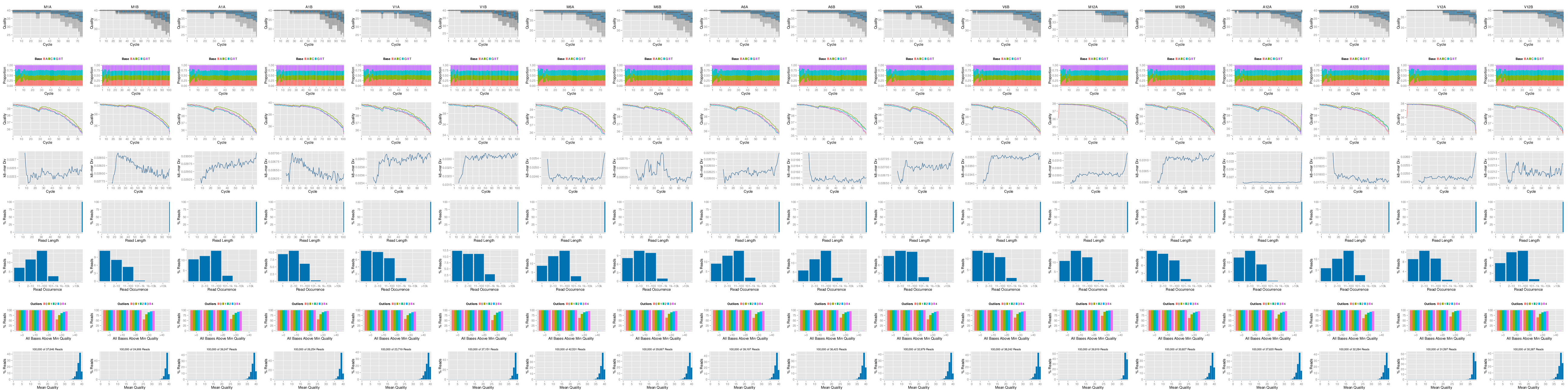
**Figure 2:** FASTQ quality report
[Back to Table of Contents]()
Parallelization of QC report on single machine with multiple cores
```{r fastq_quality_parallel_single, eval=FALSE}
args <- systemArgs(sysma="param/tophat.param", mytargets="targets.txt")
f <- function(x) seeFastq(fastq=infile1(args)[x], batchsize=100000, klength=8)
fqlist <- bplapply(seq(along=args), f, BPPARAM = MulticoreParam(workers=8))
seeFastqPlot(unlist(fqlist, recursive=FALSE))
```
[Back to Table of Contents]()
Parallelization of QC report via scheduler (_e.g._ Torque) across several compute nodes
```{r fastq_quality_parallel_cluster, eval=FALSE}
library(BiocParallel); library(BatchJobs)
f <- function(x) {
library(systemPipeR)
args <- systemArgs(sysma="param/tophat.param", mytargets="targets.txt")
seeFastq(fastq=infile1(args)[x], batchsize=100000, klength=8)
}
funs <- makeClusterFunctionsTorque("torque.tmpl")
param <- BatchJobsParam(length(args), resources=list(walltime="20:00:00", nodes="1:ppn=1", memory="6gb"), cluster.functions=funs)
register(param)
fqlist <- bplapply(seq(along=args), f)
seeFastqPlot(unlist(fqlist, recursive=FALSE))
```
[Back to Table of Contents]()
## Alignment with _`Tophat2`_
Build _`Bowtie2`_ index.
```{r bowtie_index, eval=FALSE}
args <- systemArgs(sysma="param/tophat.param", mytargets="targets.txt")
moduleload(modules(args)) # Skip if module system is not available
system("bowtie2-build ./data/tair10.fasta ./data/tair10.fasta")
```
Execute _`SYSargs`_ on a single machine without submitting to a queuing system of a compute cluster. This way the input FASTQ files will be processed sequentially. If available, multiple CPU cores can be used for processing each file. The number of CPU cores (here 4) to use for each process is defined in the _`*.param`_ file. With _`cores(args)`_ one can return this value from the _`SYSargs`_ object. Note, if a module system is not installed or used, then the corresponding _`*.param`_ file needs to be edited accordingly by either providing an empty field in the line(s) starting with _`module`_ or by deleting these lines.
```{r run_bowtie_single, eval=FALSE}
bampaths <- runCommandline(args=args)
```
Alternatively, the computation can be greatly accelerated by processing many files in parallel using several compute nodes of a cluster, where a scheduling/queuing system is used for load balancing. To avoid over-subscription of CPU cores on the compute nodes, the value from _`cores(args)`_ is passed on to the submission command, here _`nodes`_ in the _`resources`_ list object. The number of independent parallel cluster processes is defined under the _`Njobs`_ argument. The following example will run 18 processes in parallel using for each 4 CPU cores. If the resources available on a cluster allow to run all 18 processes at the same time then the shown sample submission will utilize in total 72 CPU cores. Note, _`clusterRun`_ can be used with most queueing systems as it is based on utilities from the _`BatchJobs`_ package which supports the use of template files (_`*.tmpl`_) for defining the run parameters of different schedulers. To run the following code, one needs to have both a conf file (see _`.BatchJob`_ samples [here](https://code.google.com/p/batchjobs/wiki/DortmundUsage)) and a template file (see _`*.tmpl`_ samples [here](https://github.com/tudo-r/BatchJobs/tree/master/examples)) for the queueing available on a system. The following example uses the sample conf and template files for the Torque scheduler provided by this package.
```{r run_bowtie_parallel, eval=FALSE}
resources <- list(walltime="20:00:00", nodes=paste0("1:ppn=", cores(args)), memory="10gb")
reg <- clusterRun(args, conffile=".BatchJobs.R", template="torque.tmpl", Njobs=18, runid="01",
resourceList=resources)
waitForJobs(reg)
```
Useful commands for monitoring progress of submitted jobs
```{r process_monitoring, eval=FALSE}
showStatus(reg)
file.exists(outpaths(args))
sapply(1:length(args), function(x) loadResult(reg, x)) # Works after job completion
```
[Back to Table of Contents]()
## Read and alignment count stats
Generate table of read and alignment counts for all samples.
```{r align_stats1, eval=FALSE}
read_statsDF <- alignStats(args)
write.table(read_statsDF, "results/alignStats.xls", row.names=FALSE, quote=FALSE, sep="\t")
```
The following shows the first four lines of the sample alignment stats file provided by the _`systemPipeR`_ package. For simplicity the number of PE reads is multiplied here by 2 to approximate proper alignment frequencies where each read in a pair is counted.
```{r align_stats2, eval=TRUE}
read.table(system.file("extdata", "alignStats.xls", package="systemPipeR"), header=TRUE)[1:4,]
```
Parallelization of read/alignment stats on single machine with multiple cores
```{r align_stats_parallel, eval=FALSE}
f <- function(x) alignStats(args[x])
read_statsList <- bplapply(seq(along=args), f, BPPARAM = MulticoreParam(workers=8))
read_statsDF <- do.call("rbind", read_statsList)
```
Parallelization of read/alignment stats via scheduler (_e.g._ Torque) across several compute nodes
```{r align_stats_parallel_cluster, eval=FALSE}
library(BiocParallel); library(BatchJobs)
f <- function(x) {
library(systemPipeR)
args <- systemArgs(sysma="tophat.param", mytargets="targets.txt")
alignStats(args[x])
}
funs <- makeClusterFunctionsTorque("torque.tmpl")
param <- BatchJobsParam(length(args), resources=list(walltime="20:00:00", nodes="1:ppn=1", memory="6gb"), cluster.functions=funs)
register(param)
read_statsList <- bplapply(seq(along=args), f)
read_statsDF <- do.call("rbind", read_statsList)
```
[Back to Table of Contents]()
## Create symbolic links for viewing BAM files in IGV
The genome browser IGV supports reading of indexed/sorted BAM files via web URLs. This way it can be avoided to create unnecessary copies of these large files. To enable this approach, an HTML directory with http access needs to be available in the user account (_e.g._ _`home/publichtml`_) of a system. If this is not the case then the BAM files need to be moved or copied to the system where IGV runs. In the following, _`htmldir`_ defines the path to the HTML directory with http access where the symbolic links to the BAM files will be stored. The corresponding URLs will be written to a text file specified under the `_urlfile`_ argument.
```{r igv, eval=FALSE}
symLink2bam(sysargs=args, htmldir=c("~/.html/", "somedir/"),
urlbase="http://myserver.edu/~username/",
urlfile="IGVurl.txt")
```
[Back to Table of Contents]()
## Alternative NGS Aligners
### Alignment with _`Bowtie2`_ (_e.g._ for miRNA profiling)
The following example runs _`Bowtie2`_ as a single process without submitting it to a cluster.
```{r bowtie2, eval=FALSE}
args <- systemArgs(sysma="bowtieSE.param", mytargets="targets.txt")
moduleload(modules(args)) # Skip if module system is not available
bampaths <- runCommandline(args=args)
```
Alternatively, submit the job to compute nodes.
```{r bowtie2_cluster, eval=FALSE}
resources <- list(walltime="20:00:00", nodes=paste0("1:ppn=", cores(args)), memory="10gb")
reg <- clusterRun(args, conffile=".BatchJobs.R", template="torque.tmpl", Njobs=18, runid="01",
resourceList=resources)
waitForJobs(reg)
```
[Back to Table of Contents]()
### Alignment with _`BWA-MEM`_ (_e.g._ for VAR-Seq)
The following example runs BWA-MEM as a single process without submitting it to a cluster.
```{r bwamem_cluster, eval=FALSE}
args <- systemArgs(sysma="param/bwa.param", mytargets="targets.txt")
moduleload(modules(args)) # Skip if module system is not available
system("bwa index -a bwtsw ./data/tair10.fasta") # Indexes reference genome
bampaths <- runCommandline(args=args[1:2])
```
[Back to Table of Contents]()
### Alignment with _`Rsubread`_ (_e.g._ for RNA-Seq)
The following example shows how one can use within the \Rpackage{systemPipeR} environment the R-based
aligner \Rpackage{Rsubread} or other R-based functions that read from input files and write to output files.
```{r rsubread, eval=FALSE}
library(Rsubread)
args <- systemArgs(sysma="param/rsubread.param", mytargets="targets.txt")
buildindex(basename=reference(args), reference=reference(args)) # Build indexed reference genome
align(index=reference(args), readfile1=infile1(args)[1:4], input_format="FASTQ",
output_file=outfile1(args)[1:4], output_format="SAM", nthreads=8, indels=1, TH1=2)
for(i in seq(along=outfile1(args))) asBam(file=outfile1(args)[i], destination=gsub(".sam", "", outfile1(args)[i]), overwrite=TRUE, indexDestination=TRUE)
```
[Back to Table of Contents]()
### Alignment with _`gsnap`_ (_e.g._ for VAR-Seq and RNA-Seq)
Another R-based short read aligner is _`gsnap`_ from the _`gmapR`_ package [@Wu2010-iq].
The code sample below introduces how to run this aligner on multiple nodes of a compute cluster.
```{r gsnap, eval=FALSE}
library(gmapR); library(BiocParallel); library(BatchJobs)
args <- systemArgs(sysma="param/gsnap.param", mytargets="targetsPE.txt")
gmapGenome <- GmapGenome(reference(args), directory="data", name="gmap_tair10chr/", create=TRUE)
f <- function(x) {
library(gmapR); library(systemPipeR)
args <- systemArgs(sysma="gsnap.param", mytargets="targetsPE.txt")
gmapGenome <- GmapGenome(reference(args), directory="data", name="gmap_tair10chr/", create=FALSE)
p <- GsnapParam(genome=gmapGenome, unique_only=TRUE, molecule="DNA", max_mismatches=3)
o <- gsnap(input_a=infile1(args)[x], input_b=infile2(args)[x], params=p, output=outfile1(args)[x])
}
funs <- makeClusterFunctionsTorque("torque.tmpl")
param <- BatchJobsParam(length(args), resources=list(walltime="20:00:00", nodes="1:ppn=1", memory="6gb"), cluster.functions=funs)
register(param)
d <- bplapply(seq(along=args), f)
```
[Back to Table of Contents]()
## Read counting for mRNA profiling experiments
Create _`txdb`_ (needs to be done only once)
```{r create_txdb, eval=FALSE}
library(GenomicFeatures)
txdb <- makeTxDbFromGFF(file="data/tair10.gff", format="gff", dataSource="TAIR", organism="A. thaliana")
saveDb(txdb, file="./data/tair10.sqlite")
```
[Back to Table of Contents]()
The following performs read counting with _`summarizeOverlaps`_ in parallel mode with multiple cores.
```{r read_counting_multicore, eval=FALSE}
library(BiocParallel)
txdb <- loadDb("./data/tair10.sqlite")
eByg <- exonsBy(txdb, by="gene")
bfl <- BamFileList(outpaths(args), yieldSize=50000, index=character())
multicoreParam <- MulticoreParam(workers=4); register(multicoreParam); registered()
counteByg <- bplapply(bfl, function(x) summarizeOverlaps(eByg, x, mode="Union", ignore.strand=TRUE, inter.feature=TRUE, singleEnd=TRUE)) # Note: for strand-specific RNA-Seq set 'ignore.strand=FALSE' and for PE data set 'singleEnd=FALSE'
countDFeByg <- sapply(seq(along=counteByg), function(x) assays(counteByg[[x]])$counts)
rownames(countDFeByg) <- names(rowRanges(counteByg[[1]])); colnames(countDFeByg) <- names(bfl)
rpkmDFeByg <- apply(countDFeByg, 2, function(x) returnRPKM(counts=x, ranges=eByg))
write.table(countDFeByg, "results/countDFeByg.xls", col.names=NA, quote=FALSE, sep="\t")
write.table(rpkmDFeByg, "results/rpkmDFeByg.xls", col.names=NA, quote=FALSE, sep="\t")
```
Please note, in addition to read counts this step generates RPKM normalized expression values. For most statistical differential expression or abundance analysis methods, such as _`edgeR`_ or _`DESeq2`_, the raw count values should be used as input. The usage of RPKM values should be restricted to specialty applications required by some users, _e.g._ manually comparing the expression levels of different genes or features.
[Back to Table of Contents]()
Read counting with _`summarizeOverlaps`_ using multiple nodes of a cluster
```{r read_counting_multinode, eval=FALSE}
library(BiocParallel)
f <- function(x) {
library(systemPipeR); library(BiocParallel); library(GenomicFeatures)
txdb <- loadDb("./data/tair10.sqlite")
eByg <- exonsBy(txdb, by="gene")
args <- systemArgs(sysma="tophat.param", mytargets="targets.txt")
bfl <- BamFileList(outpaths(args), yieldSize=50000, index=character())
summarizeOverlaps(eByg, bfl[x], mode="Union", ignore.strand=TRUE, inter.feature=TRUE, singleEnd=TRUE)
}
funs <- makeClusterFunctionsTorque("torque.tmpl")
param <- BatchJobsParam(length(args), resources=list(walltime="20:00:00", nodes="1:ppn=1", memory="6gb"), cluster.functions=funs)
register(param)
counteByg <- bplapply(seq(along=args), f)
countDFeByg <- sapply(seq(along=counteByg), function(x) assays(counteByg[[x]])$counts)
rownames(countDFeByg) <- names(rowRanges(counteByg[[1]])); colnames(countDFeByg) <- names(outpaths(args))
```
[Back to Table of Contents]()
## Read counting for miRNA profiling experiments
Download miRNA genes from miRBase
```{r read_counting_mirna, eval=FALSE}
system("wget ftp://mirbase.org/pub/mirbase/19/genomes/My_species.gff3 -P ./data/")
gff <- import.gff("./data/My_species.gff3")
gff <- split(gff, elementMetadata(gff)$ID)
bams <- names(bampaths); names(bams) <- targets$SampleName
bfl <- BamFileList(bams, yieldSize=50000, index=character())
countDFmiR <- summarizeOverlaps(gff, bfl, mode="Union", ignore.strand=FALSE, inter.feature=FALSE) # Note: inter.feature=FALSE important since pre and mature miRNA ranges overlap
rpkmDFmiR <- apply(countDFmiR, 2, function(x) returnRPKM(counts=x, gffsub=gff))
write.table(assays(countDFmiR)$counts, "results/countDFmiR.xls", col.names=NA, quote=FALSE, sep="\t")
write.table(rpkmDFmiR, "results/rpkmDFmiR.xls", col.names=NA, quote=FALSE, sep="\t")
```
[Back to Table of Contents]()
## Correlation analysis of samples
The following computes the sample-wise Spearman correlation coefficients from the _`rlog`_ (regularized-logarithm) transformed expression values generated with the _`DESeq2`_ package. After transformation to a distance matrix, hierarchical clustering is performed with the _`hclust`_ function and the result is plotted as a dendrogram ([sample\_tree.pdf](./results/sample_tree.pdf)).
```{r sample_tree_rlog, eval=TRUE}
library(DESeq2, warn.conflicts=FALSE, quietly=TRUE); library(ape, warn.conflicts=FALSE)
countDFpath <- system.file("extdata", "countDFeByg.xls", package="systemPipeR")
countDF <- as.matrix(read.table(countDFpath))
colData <- data.frame(row.names=targetsin(args)$SampleName, condition=targetsin(args)$Factor)
dds <- DESeqDataSetFromMatrix(countData = countDF, colData = colData, design = ~ condition)
d <- cor(assay(rlog(dds)), method="spearman")
hc <- hclust(dist(1-d))
plot.phylo(as.phylo(hc), type="p", edge.col=4, edge.width=3, show.node.label=TRUE, no.margin=TRUE)
```
**Figure 3:** Correlation dendrogram of samples for _`rlog`_ values.
Alternatively, the clustering can be performed with _`RPKM`_ normalized expression values. In combination with Spearman correlation the results of the two clustering methods are often relatively similar.
```{r sample_tree_rpkm, eval=FALSE}
rpkmDFeBygpath <- system.file("extdata", "rpkmDFeByg.xls", package="systemPipeR")
rpkmDFeByg <- read.table(rpkmDFeBygpath, check.names=FALSE)
rpkmDFeByg <- rpkmDFeByg[rowMeans(rpkmDFeByg) > 50,]
d <- cor(rpkmDFeByg, method="spearman")
hc <- hclust(as.dist(1-d))
plot.phylo(as.phylo(hc), type="p", edge.col="blue", edge.width=2, show.node.label=TRUE, no.margin=TRUE)
```
[Back to Table of Contents]()
## DEG analysis with _`edgeR`_
The following _`run_edgeR`_ function is a convenience wrapper for
identifying differentially expressed genes (DEGs) in batch mode with
_`edgeR`_'s GML method [@Robinson2010-uk] for any number of
pairwise sample comparisons specified under the _`cmp`_ argument. Users
are strongly encouraged to consult the
[_`edgeR`_](\href{http://www.bioconductor.org/packages/devel/bioc/vignettes/edgeR/inst/doc/edgeRUsersGuide.pdf) vignette
for more detailed information on this topic and how to properly run _`edgeR`_
on data sets with more complex experimental designs.
```{r edger_wrapper, eval=TRUE}
targets <- read.delim(targetspath, comment="#")
cmp <- readComp(file=targetspath, format="matrix", delim="-")
cmp[[1]]
countDFeBygpath <- system.file("extdata", "countDFeByg.xls", package="systemPipeR")
countDFeByg <- read.delim(countDFeBygpath, row.names=1)
edgeDF <- run_edgeR(countDF=countDFeByg, targets=targets, cmp=cmp[[1]], independent=FALSE, mdsplot="")
```
Filter and plot DEG results for up and down regulated genes. Because of the small size of the toy data set used by this vignette, the _FDR_ value has been set to a relatively high threshold (here 10%). More commonly used _FDR_ cutoffs are 1% or 5%. The definition of '_up_' and '_down_' is given in the corresponding help file. To open it, type _`?filterDEGs`_ in the R console.
```{r edger_deg_counts, eval=TRUE}
DEG_list <- filterDEGs(degDF=edgeDF, filter=c(Fold=2, FDR=10))
```
**Figure 4:** Up and down regulated DEGs identified by _`edgeR`_.
```{r edger_deg_stats, eval=TRUE}
names(DEG_list)
DEG_list$Summary[1:4,]
```
[Back to Table of Contents]()
## DEG analysis with _`DESeq2`_
The following _`run_DESeq2`_ function is a convenience wrapper for
identifying DEGs in batch mode with _`DESeq2`_ [@Love2014-sh] for any number of
pairwise sample comparisons specified under the _`cmp`_ argument. Users
are strongly encouraged to consult the
[_`DESeq2`_](http://www.bioconductor.org/packages/devel/bioc/vignettes/DESeq2/inst/doc/DESeq2.pdf) vignette
for more detailed information on this topic and how to properly run _`DESeq2`_
on data sets with more complex experimental designs.
```{r deseq2_wrapper, eval=TRUE}
degseqDF <- run_DESeq2(countDF=countDFeByg, targets=targets, cmp=cmp[[1]], independent=FALSE)
```
Filter and plot DEG results for up and down regulated genes.
```{r deseq2_deg_counts, eval=TRUE}
DEG_list2 <- filterDEGs(degDF=degseqDF, filter=c(Fold=2, FDR=10))
```
**Figure 5:** Up and down regulated DEGs identified by _`DESeq2`_.
[Back to Table of Contents]()
## Venn Diagrams
The function _`overLapper`_ can compute Venn intersects for large numbers of sample sets (up to 20 or more) and _`vennPlot`_ can plot 2-5 way Venn diagrams. A useful feature is the possiblity to combine the counts from several Venn comparisons with the same number of sample sets in a single Venn diagram (here for 4 up and down DEG sets).
```{r vennplot, eval=TRUE}
vennsetup <- overLapper(DEG_list$Up[6:9], type="vennsets")
vennsetdown <- overLapper(DEG_list$Down[6:9], type="vennsets")
vennPlot(list(vennsetup, vennsetdown), mymain="", mysub="", colmode=2, ccol=c("blue", "red"))
```
**Figure 6:** Venn Diagram for 4 Up and Down DEG Sets.
[Back to Table of Contents]()
## GO term enrichment analysis of DEGs
### Obtain gene-to-GO mappings
The following shows how to obtain gene-to-GO mappings from _`biomaRt`_ (here for _A. thaliana_) and how to organize them for the downstream GO term enrichment analysis. Alternatively, the gene-to-GO mappings can be obtained for many organisms from Bioconductor's _`*.db`_ genome annotation packages or GO annotation files provided by various genome databases. For each annotation this relatively slow preprocessing step needs to be performed only once. Subsequently, the preprocessed data can be loaded with the _`load`_ function as shown in the next subsection.
```{r get_go_biomart, eval=FALSE}
library("biomaRt")
listMarts() # To choose BioMart database
m <- useMart("ENSEMBL_MART_PLANT"); listDatasets(m)
m <- useMart("ENSEMBL_MART_PLANT", dataset="athaliana_eg_gene")
listAttributes(m) # Choose data types you want to download
go <- getBM(attributes=c("go_accession", "tair_locus", "go_namespace_1003"), mart=m)
go <- go[go[,3]!="",]; go[,3] <- as.character(go[,3])
dir.create("./data/GO")
write.table(go, "data/GO/GOannotationsBiomart_mod.txt", quote=FALSE, row.names=FALSE, col.names=FALSE, sep="\t")
catdb <- makeCATdb(myfile="data/GO/GOannotationsBiomart_mod.txt", lib=NULL, org="", colno=c(1,2,3), idconv=NULL)
save(catdb, file="data/GO/catdb.RData")
```
[Back to Table of Contents]()
### Batch GO term enrichment analysis
Apply the enrichment analysis to the DEG sets obtained in the above differential expression analysis. Note, in the following example the _FDR_ filter is set here to an unreasonably high value, simply because of the small size of the toy data set used in this vignette. Batch enrichment analysis of many gene sets is performed with the _`GOCluster_Report`_ function. When _`method="all"`_, it returns all GO terms passing the p-value cutoff specified under the _`cutoff`_ arguments. When _`method="slim"`_, it returns only the GO terms specified under the _`myslimv`_ argument. The given example shows how one can obtain such a GO slim vector from BioMart for a specific organism.
```{r go_enrichment, eval=FALSE}
load("data/GO/catdb.RData")
DEG_list <- filterDEGs(degDF=edgeDF, filter=c(Fold=2, FDR=50), plot=FALSE)
up_down <- DEG_list$UporDown; names(up_down) <- paste(names(up_down), "_up_down", sep="")
up <- DEG_list$Up; names(up) <- paste(names(up), "_up", sep="")
down <- DEG_list$Down; names(down) <- paste(names(down), "_down", sep="")
DEGlist <- c(up_down, up, down)
DEGlist <- DEGlist[sapply(DEGlist, length) > 0]
BatchResult <- GOCluster_Report(catdb=catdb, setlist=DEGlist, method="all", id_type="gene", CLSZ=2, cutoff=0.9, gocats=c("MF", "BP", "CC"), recordSpecGO=NULL)
library("biomaRt"); m <- useMart("ENSEMBL_MART_PLANT", dataset="athaliana_eg_gene")
goslimvec <- as.character(getBM(attributes=c("goslim_goa_accession"), mart=m)[,1])
BatchResultslim <- GOCluster_Report(catdb=catdb, setlist=DEGlist, method="slim", id_type="gene", myslimv=goslimvec, CLSZ=10, cutoff=0.01, gocats=c("MF", "BP", "CC"), recordSpecGO=NULL)
```
[Back to Table of Contents]()
### Plot batch GO term results
The _`data.frame`_ generated by _`GOCluster_Report`_ can be plotted with the _`goBarplot`_ function. Because of the variable size of the sample sets, it may not always be desirable to show the results from different DEG sets in the same bar plot. Plotting single sample sets is achieved by subsetting the input data frame as shown in the first line of the following example.
```{r plot_go_enrichment, eval=FALSE}
gos <- BatchResultslim[grep("M6-V6_up_down", BatchResultslim$CLID), ]
gos <- BatchResultslim
pdf("GOslimbarplotMF.pdf", height=8, width=10); goBarplot(gos, gocat="MF"); dev.off()
goBarplot(gos, gocat="BP")
goBarplot(gos, gocat="CC")
```
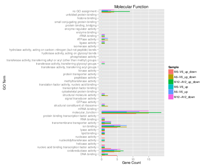
**Figure 7:** GO Slim Barplot for MF Ontology.
[Back to Table of Contents]()
## Clustering and heat maps
The following example performs hierarchical clustering on the _`rlog`_ transformed expression matrix subsetted by the DEGs identified in the
above differential expression analysis. It uses a Pearson correlation-based distance measure and complete linkage for cluster joining.
```{r hierarchical_clustering, eval=FALSE}
library(pheatmap)
geneids <- unique(as.character(unlist(DEG_list[[1]])))
y <- assay(rlog(dds))[geneids, ]
pdf("heatmap1.pdf")
pheatmap(y, scale="row", clustering_distance_rows="correlation", clustering_distance_cols="correlation")
dev.off()
```
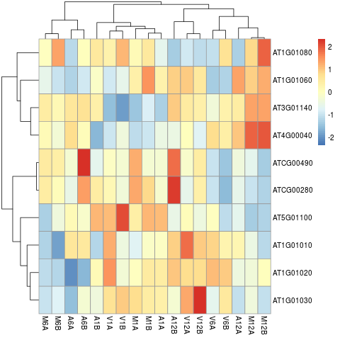
**Figure 8:** Heat map with hierarchical clustering dendrograms of DEGs.
[Back to Table of Contents]()
# Workflow templates
## RNA-Seq sample
Load the RNA-Seq sample workflow into your current working directory.
```{r genRna_workflow_single, eval=FALSE}
library(systemPipeRdata)
genWorkenvir(workflow="rnaseq")
setwd("rnaseq")
```
[Back to Table of Contents]()
### Run workflow
Next, run the chosen sample workflow _`systemPipeRNAseq`_ ([PDF](https://github.com/tgirke/systemPipeRdata/blob/master/inst/extdata/workflows/rnaseq/systemPipeRNAseq.pdf?raw=true), [Rnw](https://github.com/tgirke/systemPipeRdata/blob/master/inst/extdata/workflows/rnaseq/systemPipeRNAseq_single.Rnw)) by executing from the command-line _`make -B`_ within the _`rnaseq`_ directory. Alternatively, one can run the code from the provided _`*.Rnw`_ template file from within R interactively.
Workflow includes following steps:
1. Read preprocessing
+ Quality filtering (trimming)
+ FASTQ quality report
2. Alignments: _`Tophat2`_ (or any other RNA-Seq aligner)
3. Alignment stats
4. Read counting
5. Sample-wise correlation analysis
6. Analysis of differentially expressed genes (DEGs)
7. GO term enrichment analysis
8. Gene-wise clustering
[Back to Table of Contents]()
## ChIP-Seq sample
Load the ChIP-Seq sample workflow into your current working directory.
```{r genChip_workflow_single, eval=FALSE}
library(systemPipeRdata)
genWorkenvir(workflow="chipseq")
setwd("chipseq")
```
[Back to Table of Contents]()
### Run workflow
Next, run the chosen sample workflow _`systemPipeChIPseq_single`_ ([PDF](https://github.com/tgirke/systemPipeRdata/blob/master/inst/extdata/workflows/chipseq/systemPipeChIPseq.pdf?raw=true), [Rnw](https://github.com/tgirke/systemPipeRdata/blob/master/inst/extdata/workflows/chipseq/systemPipeChIPseq_single.Rnw)) by executing from the command-line _`make -B`_ within the _`chipseq`_ directory. Alternatively, one can run the code from the provided _`*.Rnw`_ template file from within R interactively.
Workflow includes following steps:
1. Read preprocessing
+ Quality filtering (trimming)
+ FASTQ quality report
2. Alignments: _`Bowtie2`_ or _`rsubread`_
3. Alignment stats
4. Peak calling: _`MACS2`_, _`BayesPeak`_
5. Peak annotation with genomic context
6. Differential binding analysis
7. GO term enrichment analysis
8. Motif analysis
[Back to Table of Contents]()
## VAR-Seq sample
### VAR-Seq workflow for single machine
Load the VAR-Seq sample workflow into your current working directory.
```{r genVar_workflow_single, eval=FALSE}
library(systemPipeRdata)
genWorkenvir(workflow="varseq")
setwd("varseq")
```
[Back to Table of Contents]()
### Run workflow
Next, run the chosen sample workflow _`systemPipeVARseq_single`_ ([PDF](https://github.com/tgirke/systemPipeRdata/blob/master/inst/extdata/workflows/varseq/systemPipeVARseq_single.pdf?raw=true), [Rnw](https://github.com/tgirke/systemPipeRdata/blob/master/inst/extdata/workflows/varseq/systemPipeVARseq_single.Rnw)) by executing from the command-line _`make -B`_ within the _`varseq`_ directory. Alternatively, one can run the code from the provided _`*.Rnw`_ template file from within R interactively.
Workflow includes following steps:
1. Read preprocessing
+ Quality filtering (trimming)
+ FASTQ quality report
2. Alignments: _`gsnap`_, _`bwa`_
3. Variant calling: _`VariantTools`_, _`GATK`_, _`BCFtools`_
4. Variant filtering: _`VariantTools`_ and _`VariantAnnotation`_
5. Variant annotation: _`VariantAnnotation`_
6. Combine results from many samples
7. Summary statistics of samples
[Back to Table of Contents]()
### VAR-Seq workflow for computer cluster
The workflow template provided for this step is called _`systemPipeVARseq.Rnw`_ ([PDF](https://github.com/tgirke/systemPipeRdata/blob/master/inst/extdata/workflows/varseq/systemPipeVARseq.pdf?raw=true), [Rnw](https://github.com/tgirke/systemPipeRdata/blob/master/inst/extdata/workflows/varseq/systemPipeVARseq.Rnw)).
It runs the above VAR-Seq workflow in parallel on multiple computer nodes of an HPC system using Torque as scheduler.
[Back to Table of Contents]()
## Ribo-Seq sample
Load the Ribo-Seq sample workflow into your current working directory.
```{r genRibo_workflow_single, eval=FALSE}
library(systemPipeRdata)
genWorkenvir(workflow="riboseq")
setwd("riboseq")
```
[Back to Table of Contents]()
### Run workflow
Next, run the chosen sample workflow _`systemPipeRIBOseq`_ ([PDF](https://github.com/tgirke/systemPipeRdata/blob/master/inst/extdata/workflows/riboseq/systemPipeRIBOseq.pdf?raw=true), [Rnw](https://github.com/tgirke/systemPipeRdata/blob/master/inst/extdata/workflows/ribseq/systemPipeRIBOseq_single.Rnw)) by executing from the command-line _`make -B`_ within the _`ribseq`_ directory. Alternatively, one can run the code from the provided _`*.Rnw`_ template file from within R interactively.
Workflow includes following steps:
1. Read preprocessing
+ Adaptor trimming and quality filtering
+ FASTQ quality report
2. Alignments: _`Tophat2`_ (or any other RNA-Seq aligner)
3. Alignment stats
4. Compute read distribution across genomic features
5. Adding custom features to workflow (e.g. uORFs)
6. Genomic read coverage along transcripts
7. Read counting
8. Sample-wise correlation analysis
9. Analysis of differentially expressed genes (DEGs)
10. GO term enrichment analysis
11. Gene-wise clustering
12. Differential ribosome binding (translational efficiency)
[Back to Table of Contents]()
# Version information
```{r sessionInfo}
sessionInfo()
```
[Back to Table of Contents]()
# References