Cartesian coordinates

The Cartesian coordinate system is the most familiar, and common, type of coordinate system. Setting limits on the coordinate system will zoom the plot (like you're looking at it with a magnifying glass), and will not change the underlying data like setting limits on a scale will.

coord_cartesian(xlim = NULL, ylim = NULL, expand = TRUE)

Arguments

xlim, ylim	Limits for the x and y axes.
expand	If TRUE, the default, adds a small expansion factor to the limits to ensure that data and axes don't overlap. If FALSE, limits are taken exactly from the data or xlim/ylim.

Examples

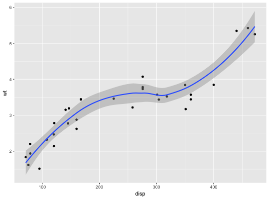
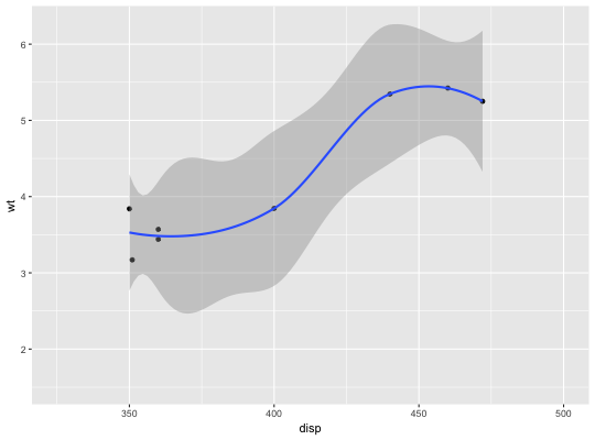
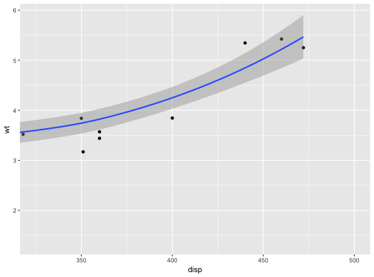
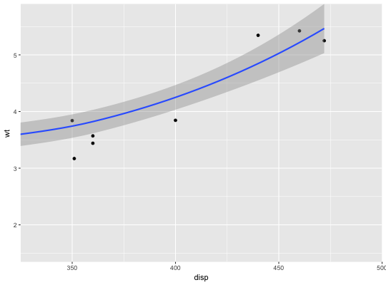
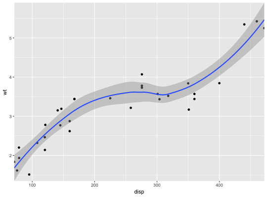
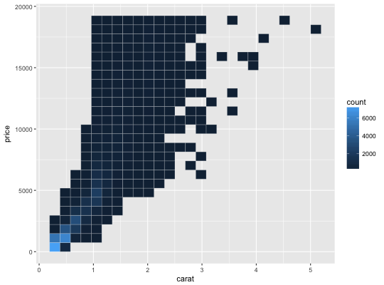
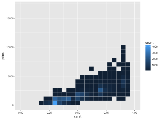
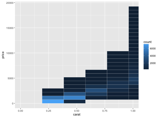
# There are two ways of zooming the plot display: with scales or
# with coordinate systems.  They work in two rather different ways.

p <- ggplot(mtcars, aes(disp, wt)) +
  geom_point() +
  geom_smooth()
p
#> `geom_smooth()` using method = 'loess' and formula 'y ~ x'

# Setting the limits on a scale converts all values outside the range to NA.
p + scale_x_continuous(limits = c(325, 500))
#> `geom_smooth()` using method = 'loess' and formula 'y ~ x'
#> Warning: Removed 24 rows containing non-finite values (stat_smooth).
#> Warning: Removed 24 rows containing missing values (geom_point).

# Setting the limits on the coordinate system performs a visual zoom.
# The data is unchanged, and we just view a small portion of the original
# plot. Note how smooth continues past the points visible on this plot.
p + coord_cartesian(xlim = c(325, 500))
#> `geom_smooth()` using method = 'loess' and formula 'y ~ x'

# By default, the same expansion factor is applied as when setting scale
# limits. You can set the limits precisely by setting expand = FALSE
p + coord_cartesian(xlim = c(325, 500), expand = FALSE)
#> `geom_smooth()` using method = 'loess' and formula 'y ~ x'

# Simiarly, we can use expand = FALSE to turn off expansion with the
# default limits
p + coord_cartesian(expand = FALSE)
#> `geom_smooth()` using method = 'loess' and formula 'y ~ x'

# You can see the same thing with this 2d histogram
d <- ggplot(diamonds, aes(carat, price)) +
  stat_bin2d(bins = 25, colour = "white")
d

# When zooming the scale, the we get 25 new bins that are the same
# size on the plot, but represent smaller regions of the data space
d + scale_x_continuous(limits = c(0, 1))
#> Warning: Removed 17502 rows containing non-finite values (stat_bin2d).

# When zooming the coordinate system, we see a subset of original 50 bins,
# displayed bigger
d + coord_cartesian(xlim = c(0, 1))