Rectangles

geom_rect and geom_tile do the same thing, but are parameterised differently: geom_rect uses the locations of the four corners (xmin, xmax, ymin and ymax), while geom_tile uses the center of the tile and its size (x, y, width, height). geom_raster is a high performance special case for when all the tiles are the same size.

geom_raster(mapping = NULL, data = NULL, stat = "identity",
  position = "identity", ..., hjust = 0.5, vjust = 0.5,
  interpolate = FALSE, na.rm = FALSE, show.legend = NA,
  inherit.aes = TRUE)

geom_rect(mapping = NULL, data = NULL, stat = "identity",
  position = "identity", ..., na.rm = FALSE, show.legend = NA,
  inherit.aes = TRUE)

geom_tile(mapping = NULL, data = NULL, stat = "identity",
  position = "identity", ..., na.rm = FALSE, show.legend = NA,
  inherit.aes = TRUE)

Arguments

mapping	Set of aesthetic mappings created by aes or aes_. If specified and inherit.aes = TRUE (the default), it is combined with the default mapping at the top level of the plot. You must supply mapping if there is no plot mapping.
data	The data to be displayed in this layer. There are three options: If NULL, the default, the data is inherited from the plot data as specified in the call to ggplot. A data.frame, or other object, will override the plot data. All objects will be fortified to produce a data frame. See fortify for which variables will be created. A function will be called with a single argument, the plot data. The return value must be a data.frame., and will be used as the layer data.
stat	The statistical transformation to use on the data for this layer, as a string.
position	Position adjustment, either as a string, or the result of a call to a position adjustment function.
...	other arguments passed on to layer. These are often aesthetics, used to set an aesthetic to a fixed value, like color = "red" or size = 3. They may also be parameters to the paired geom/stat.
hjust, vjust	horizontal and vertical justification of the grob. Each justification value should be a number between 0 and 1. Defaults to 0.5 for both, centering each pixel over its data location.
interpolate	If TRUE interpolate linearly, if FALSE (the default) don't interpolate.
na.rm	If FALSE, the default, missing values are removed with a warning. If TRUE, missing values are silently removed.
show.legend	logical. Should this layer be included in the legends? NA, the default, includes if any aesthetics are mapped. FALSE never includes, and TRUE always includes.
inherit.aes	If FALSE, overrides the default aesthetics, rather than combining with them. This is most useful for helper functions that define both data and aesthetics and shouldn't inherit behaviour from the default plot specification, e.g. borders.

Aesthetics

geom_tile understands the following aesthetics (required aesthetics are in bold):

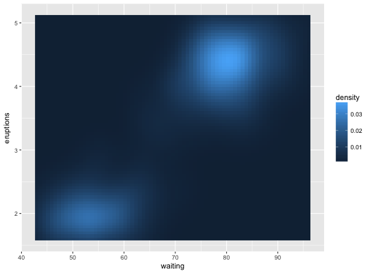
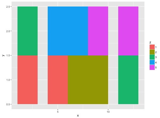
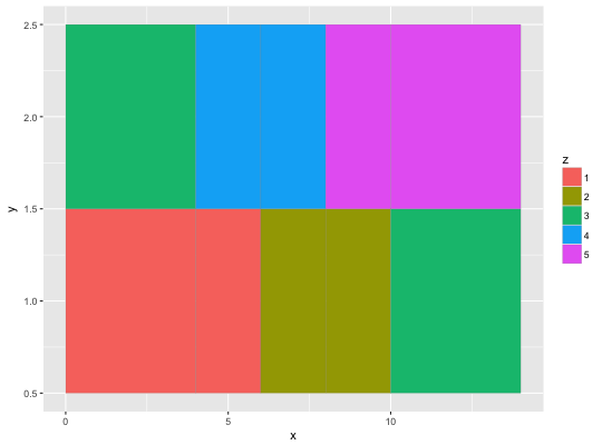
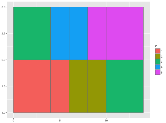
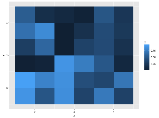
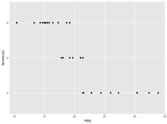
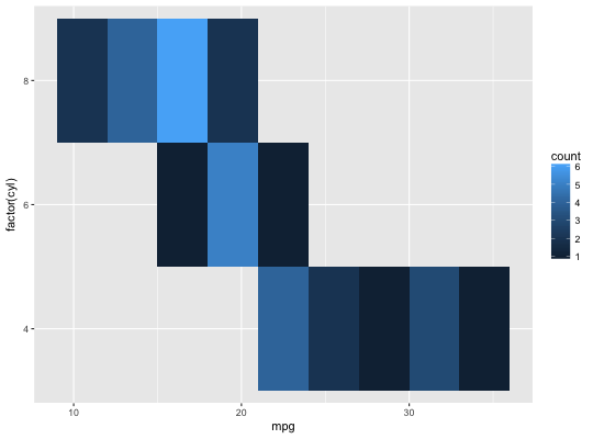
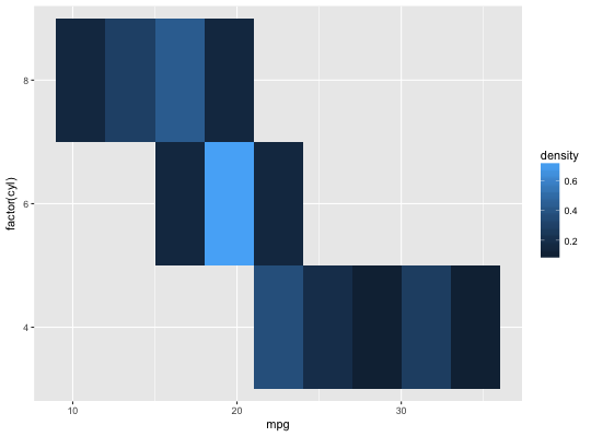
• x

• y

• alpha

• colour

• fill

• group

• linetype

• size

Examples

# The most common use for rectangles is to draw a surface. You always want
# to use geom_raster here because it's so much faster, and produces
# smaller output when saving to PDF
ggplot(faithfuld, aes(waiting, eruptions)) +
 geom_raster(aes(fill = density))

# Interpolation smooths the surface & is most helpful when rendering images.
ggplot(faithfuld, aes(waiting, eruptions)) +
 geom_raster(aes(fill = density), interpolate = TRUE)

# If you want to draw arbitrary rectangles, use geom_tile() or geom_rect()
df <- data.frame(
  x = rep(c(2, 5, 7, 9, 12), 2),
  y = rep(c(1, 2), each = 5),
  z = factor(rep(1:5, each = 2)),
  w = rep(diff(c(0, 4, 6, 8, 10, 14)), 2)
)
ggplot(df, aes(x, y)) +
  geom_tile(aes(fill = z))
ggplot(df, aes(x, y)) +
  geom_tile(aes(fill = z, width = w), colour = "grey50")
#> Warning: Ignoring unknown aesthetics: width
ggplot(df, aes(xmin = x - w / 2, xmax = x + w / 2, ymin = y, ymax = y + 1)) +
  geom_rect(aes(fill = z, width = w), colour = "grey50")
#> Warning: Ignoring unknown aesthetics: width


# Justification controls where the cells are anchored
df <- expand.grid(x = 0:5, y = 0:5)
df$z <- runif(nrow(df))
# default is compatible with geom_tile()
ggplot(df, aes(x, y, fill = z)) + geom_raster()
# zero padding
ggplot(df, aes(x, y, fill = z)) + geom_raster(hjust = 0, vjust = 0)

# Inspired by the image-density plots of Ken Knoblauch
cars <- ggplot(mtcars, aes(mpg, factor(cyl)))
cars + geom_point()
cars + stat_bin2d(aes(fill = ..count..), binwidth = c(3,1))
cars + stat_bin2d(aes(fill = ..density..), binwidth = c(3,1))

cars + stat_density(aes(fill = ..density..), geom = "raster", position = "identity")
cars + stat_density(aes(fill = ..count..), geom = "raster", position = "identity")