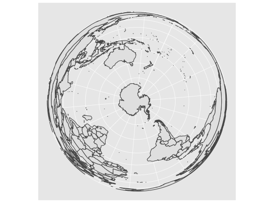
Visualise sf objects

This set geom, stat, and coord are used to visualise simple feature (sf) objects. For simple plots, you will only need geom_sf as it uses stat_sf and adds coord_sf for you. geom_sf is an unusual geom because it will draw different geometric objects depending on what simple features are present in the data: you can get points, lines, or polygons.

stat_sf(mapping = NULL, data = NULL, geom = "rect",
  position = "identity", na.rm = FALSE, show.legend = NA,
  inherit.aes = TRUE, ...)

geom_sf(mapping = aes(), data = NULL, stat = "sf",
  position = "identity", na.rm = FALSE, show.legend = NA,
  inherit.aes = TRUE, ...)

coord_sf(xlim = NULL, ylim = NULL, expand = TRUE, crs = NULL,
  datum = sf::st_crs(4326))

Arguments

mapping	Set of aesthetic mappings created by aes or aes_. If specified and inherit.aes = TRUE (the default), it is combined with the default mapping at the top level of the plot. You must supply mapping if there is no plot mapping.
data	The data to be displayed in this layer. There are three options: If NULL, the default, the data is inherited from the plot data as specified in the call to ggplot. A data.frame, or other object, will override the plot data. All objects will be fortified to produce a data frame. See fortify for which variables will be created. A function will be called with a single argument, the plot data. The return value must be a data.frame., and will be used as the layer data.
geom	The geometric object to use display the data
position	Position adjustment, either as a string, or the result of a call to a position adjustment function.
na.rm	If FALSE, the default, missing values are removed with a warning. If TRUE, missing values are silently removed.
show.legend	logical. Should this layer be included in the legends? NA, the default, includes if any aesthetics are mapped. FALSE never includes, and TRUE always includes.
inherit.aes	If FALSE, overrides the default aesthetics, rather than combining with them. This is most useful for helper functions that define both data and aesthetics and shouldn't inherit behaviour from the default plot specification, e.g. borders.
...	other arguments passed on to layer. These are often aesthetics, used to set an aesthetic to a fixed value, like color = "red" or size = 3. They may also be parameters to the paired geom/stat.
stat	The statistical transformation to use on the data for this layer, as a string.
xlim	Limits for the x and y axes.
ylim	Limits for the x and y axes.
expand	If TRUE, the default, adds a small expansion factor to the limits to ensure that data and axes don't overlap. If FALSE, limits are taken exactly from the data or xlim/ylim.
crs	Use this to select a specific CRS. If not specified, will use the CRS defined in the first layer.
datum	CRS that provides datum to use when generating graticules

Geometry aesthetic

geom_sf uses a unique aesthetic: geometry, giving an column of class sfc containg simple features data. There are three ways to supply the geometry aesthetic:

• Do nothing: by default geom_sf assumes it is stored in the geometry column.

• Explicitly pass an sf object to the data argument. This will use the primary geometry column, no matter what it's called.

• Supply your own using aes(geometry = my_column)

Unlike other aesthetics, geometry will never be inherited from the plot.

CRS

coord_sf() ensures that all layers use a common CRS. You can either specify it using the CRS param, or coord_sf will take it from the first layer that defines a CRS.

Examples

if (requireNamespace("sf", quietly = TRUE)) {
nc <- sf::st_read(system.file("shape/nc.shp", package = "sf"), quiet = TRUE)
ggplot(nc) +
  geom_sf(aes(fill = AREA))

# If not supplied, coord_sf() will take the CRS from the first layer
# and automatically transform all other layers to use that CRS. This
# ensures that all data will correctly line up
nc_3857 <- sf::st_transform(nc, "+init=epsg:3857")
ggplot() +
  geom_sf(data = nc) +
  geom_sf(data = nc_3857, colour = "red", fill = NA)

# You can also use layers with x and y aesthetics: these are
# assumed to already be in the common CRS.
ggplot(nc) +
  geom_sf() +
  annotate("point", x = -80, y = 35, colour = "red", size = 4)

# Thanks to the power of sf, ageom_sf nicely handles varying projections
# setting the aspect ratio correctly.
library(maps)
world1 <- sf::st_as_sf(map('world', plot = FALSE, fill = TRUE))
ggplot() + geom_sf(data = world1)

world2 <- sf::st_transform(
  world1,
  "+proj=laea +y_0=0 +lon_0=155 +lat_0=-90 +ellps=WGS84 +no_defs"
)
ggplot() + geom_sf(data = world2)
}