 \n",
"Creative Commons Attribution 4.0 International License. All code examples are also licensed under the [MIT license](http://opensource.org/licenses/MIT)."
]
},
{
"cell_type": "markdown",
"metadata": {
"slideshow": {
"slide_type": "slide"
}
},
"source": [
"## What is this?"
]
},
{
"cell_type": "markdown",
"metadata": {},
"source": [
"This is a gentle introduction to the IPython Notebook aimed at lecturers who wish to incorporate it in their teaching, written in an IPython Notebook. This presentation adapts material from the [IPython official documentation](http://nbviewer.ipython.org/github/ipython/ipython/blob/2.x/examples/Notebook)."
]
},
{
"cell_type": "markdown",
"metadata": {
"slideshow": {
"slide_type": "slide"
}
},
"source": [
"## What is an IPython Notebook?\n",
"\n",
"An IPython Notebook is a:\n",
"\n",
"**[A]** Interactive environment for writing and running code \n",
"**[B]** Weave of code, data, prose, equations, analysis, and visualization \n",
"**[C]** Tool for prototyping new code and analysis \n",
"**[D]** Reproducible workflow for scientific research \n",
"**[E]** All of the above"
]
},
{
"cell_type": "markdown",
"metadata": {
"slideshow": {
"slide_type": "fragment"
}
},
"source": [
"**[E]** All of the above"
]
},
{
"cell_type": "markdown",
"metadata": {
"slideshow": {
"slide_type": "slide"
}
},
"source": [
"## How Do I Open an IPython Notebook?"
]
},
{
"cell_type": "markdown",
"metadata": {},
"source": [
"Open a command prompt and execute \n",
"\n",
" ipython notebook\n",
"and an IPython Notebook server will start and launch a viewer in the default web browser. Notebooks found in the working directory will show up in the list of notebooks. "
]
},
{
"cell_type": "markdown",
"metadata": {
"slideshow": {
"slide_type": "slide"
}
},
"source": [
"## Example\n",
"\n",
"For example, navigating to the course `Lessons` directory and executing `ipython notebook` will launch a browser window similar to that shown below\n",
"\n",
"
\n",
"Creative Commons Attribution 4.0 International License. All code examples are also licensed under the [MIT license](http://opensource.org/licenses/MIT)."
]
},
{
"cell_type": "markdown",
"metadata": {
"slideshow": {
"slide_type": "slide"
}
},
"source": [
"## What is this?"
]
},
{
"cell_type": "markdown",
"metadata": {},
"source": [
"This is a gentle introduction to the IPython Notebook aimed at lecturers who wish to incorporate it in their teaching, written in an IPython Notebook. This presentation adapts material from the [IPython official documentation](http://nbviewer.ipython.org/github/ipython/ipython/blob/2.x/examples/Notebook)."
]
},
{
"cell_type": "markdown",
"metadata": {
"slideshow": {
"slide_type": "slide"
}
},
"source": [
"## What is an IPython Notebook?\n",
"\n",
"An IPython Notebook is a:\n",
"\n",
"**[A]** Interactive environment for writing and running code \n",
"**[B]** Weave of code, data, prose, equations, analysis, and visualization \n",
"**[C]** Tool for prototyping new code and analysis \n",
"**[D]** Reproducible workflow for scientific research \n",
"**[E]** All of the above"
]
},
{
"cell_type": "markdown",
"metadata": {
"slideshow": {
"slide_type": "fragment"
}
},
"source": [
"**[E]** All of the above"
]
},
{
"cell_type": "markdown",
"metadata": {
"slideshow": {
"slide_type": "slide"
}
},
"source": [
"## How Do I Open an IPython Notebook?"
]
},
{
"cell_type": "markdown",
"metadata": {},
"source": [
"Open a command prompt and execute \n",
"\n",
" ipython notebook\n",
"and an IPython Notebook server will start and launch a viewer in the default web browser. Notebooks found in the working directory will show up in the list of notebooks. "
]
},
{
"cell_type": "markdown",
"metadata": {
"slideshow": {
"slide_type": "slide"
}
},
"source": [
"## Example\n",
"\n",
"For example, navigating to the course `Lessons` directory and executing `ipython notebook` will launch a browser window similar to that shown below\n",
"\n",
"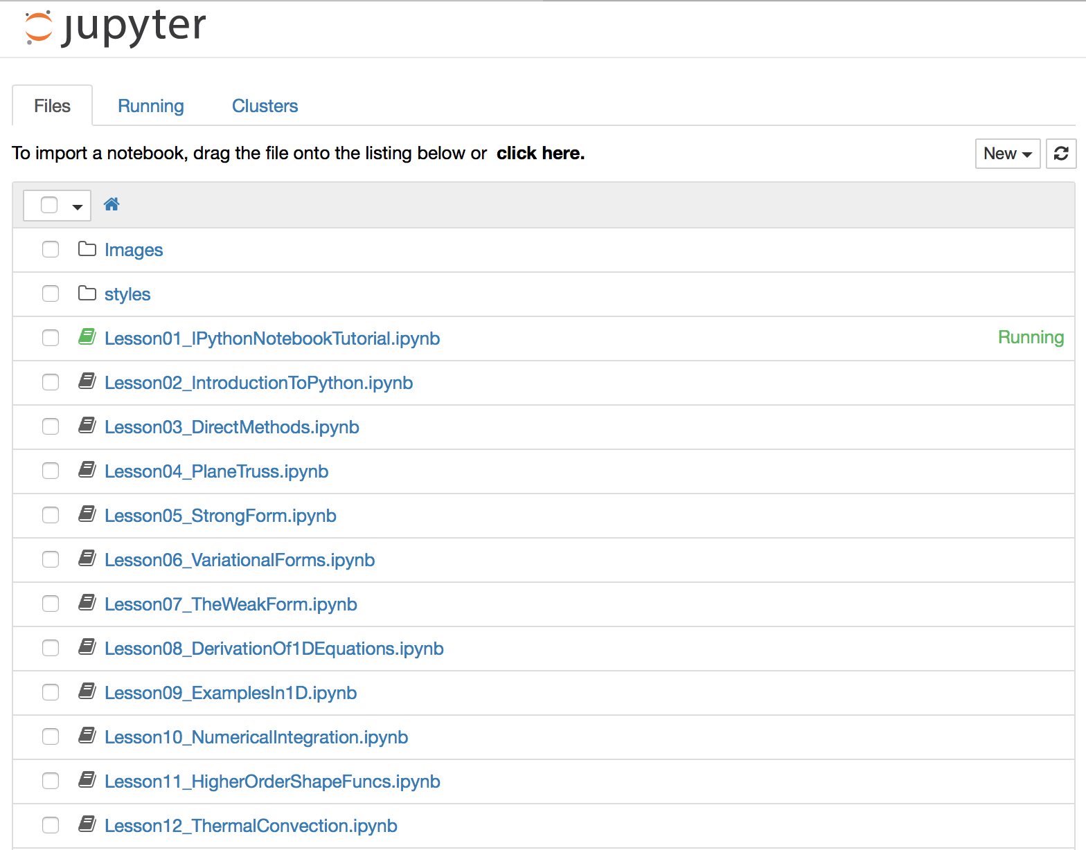 "
]
},
{
"cell_type": "markdown",
"metadata": {
"slideshow": {
"slide_type": "slide"
}
},
"source": [
"## Writing and Running Code\n",
"\n",
"The IPython Notebook consists of an ordered list of cells. \n",
"\n",
"There are three important cell types:\n",
"\n",
"* **Code**\n",
"* **Markdown**\n",
"* **Raw NBConvert**"
]
},
{
"cell_type": "markdown",
"metadata": {
"slideshow": {
"slide_type": "subslide"
}
},
"source": [
"### Code Cells"
]
},
{
"cell_type": "code",
"execution_count": 11,
"metadata": {
"collapsed": true,
"slideshow": {
"slide_type": "-"
}
},
"outputs": [],
"source": [
"# This is a code cell made up of Python comments\n",
"# We can execute it by clicking on it with the mouse\n",
"# then clicking the \"Run Cell\" button"
]
},
{
"cell_type": "code",
"execution_count": 3,
"metadata": {
"collapsed": false
},
"outputs": [
{
"name": "stdout",
"output_type": "stream",
"text": [
"Hello, World\n"
]
}
],
"source": [
"# A comment is a pretty boring piece of code\n",
"# This code cell generates \"Hello, World\" when executed\n",
"\n",
"print \"Hello, World\""
]
},
{
"cell_type": "markdown",
"metadata": {
"slideshow": {
"slide_type": "subslide"
}
},
"source": [
"### Code Cells"
]
},
{
"cell_type": "code",
"execution_count": 4,
"metadata": {
"collapsed": false,
"slideshow": {
"slide_type": "-"
}
},
"outputs": [
{
"data": {
"image/png": [
"iVBORw0KGgoAAAANSUhEUgAAAXUAAAEACAYAAABMEua6AAAABHNCSVQICAgIfAhkiAAAAAlwSFlz\n",
"AAALEgAACxIB0t1+/AAADstJREFUeJzt3X+M5PVdx/Hni7trbUNSQkjOwm1zjUBSTI1HG3qhVdZa\n",
"E3oxV/8gSmNDQ4wlRAT5w9Q2jT3/0n+MFZviqUCoVQihhlz1asXKYRuTs+39KD8OBVPiHQ1H0+vR\n",
"wqXJnX37x8zBMOzOzO7N3Hfus89HsmG+M5+deWcz99zPfHcmpKqQJLXhvK4HkCRNj1GXpIYYdUlq\n",
"iFGXpIYYdUlqiFGXpIaMjHqSn0qyN8mBJE8m+eNl1t2R5OkkB5Nsmc2okqRx1o+6sap+nOSXqupE\n",
"kvXA15O8r6q+fnpNkm3ApVV1WZL3AHcCW2c7tiRpKWNPv1TVif7FNwDrgGNDS7YD9/bX7gUuSLJx\n",
"mkNKkiYzNupJzktyADgKPFJVTw4tuQQ4PHB8BNg0vRElSZOaZKf+k6r6eXqh/sUki0ssy/C3TWE2\n",
"SdIKjTynPqiqXkzyT8C7gT0DNz0HLAwcb+pf9xpJDL0krUJVDW+clzUy6kkuAk5V1fEkbwJ+Bfij\n",
"oWW7gFuA+5NsBY5X1dEzHaxlSXZU1Y6OZ6j5eEEVup8jc/HcnIfnxbzwZ/GqlW6Ix+3U3wrcm+Q8\n",
"eqdq/raqvprkJoCq2llVu5NsS/IM8DJw42oGlySduXFvaXwMuHKJ63cOHd8y5bkkSavgJ0q7safr\n",
"ATSX9nQ9wBzZ0/UA56qcrf9JRpKah/OW6vGc+mtn8LmpebXSdrpTl6SGGHVJaohRl6SGGHVJaohR\n",
"l6SGGHVJaohRl6SGGHVJaohRl6SGGHVJaohRl6SGGHVJaohRl6SGGHVJaohRl6SGGHVJaohRl6SG\n",
"GHVJaohRl6SGGHVJaohRl6SGGHVJaohRl6SGGHVJaohRl6SGGHVJasjIqCdZSPJIkieSPJ7k1iXW\n",
"LCZ5Mcn+/tenZjeuJGmU9WNuPwncXlUHkpwPfCvJw1V1aGjdo1W1fTYjSpImNXKnXlXPV9WB/uWX\n",
"gEPAxUsszQxmkySt0MTn1JNsBrYAe4duKuDqJAeT7E5yxfTGkyStxLjTLwD0T708CNzW37EP2gcs\n",
"VNWJJB8EHgIun+6YkqRJjI16kg3AF4EvVNVDw7dX1Y8GLn85yeeSXFhVx5a4rx0Dh3uqas+qppak\n",
"RiVZBBZX/f1VNerOA9wLfL+qbl9mzUbghaqqJFcBD1TV5iXWVVV57n1OJKnembOuhe7nCD43Na9W\n",
"2s5xO/X3Ah8Bvp1kf/+6TwJvA6iqncB1wM1JTgEngOtXPLUkaSpG7tSn+kDu1OeKO/XXzuBzU/Nq\n",
"pe30E6WS1BCjLkkNMeqS1BCjLkkNMeqS1BCjLkkNMeqS1BCjLkkNMeqS1BCjLkkNMeqS1BCjLkkN\n",
"MeqS1BCjLkkNMeqS1BCjLkkNMeqS1BCjLkkNMeqS1BCjLkkNMeqS1BCjLkkNMeqS1BCjLkkNMeqS\n",
"1BCjLkkNMeqS1BCjLkkNMeqS1JCRUU+ykOSRJE8keTzJrcusuyPJ00kOJtkym1ElSeOsH3P7SeD2\n",
"qjqQ5HzgW0kerqpDpxck2QZcWlWXJXkPcCewdXYjS5KWM3KnXlXPV9WB/uWXgEPAxUPLtgP39tfs\n",
"BS5IsnEGs0qSxpj4nHqSzcAWYO/QTZcAhweOjwCbznQwSdLKjTv9AkD/1MuDwG39Hfvrlgwd1zL3\n",
"s2PgcE9V7Znk8VuTZMmfjyQlWQQWV/39VaP7kmQD8I/Al6vqM0vc/pf0An1///gp4JqqOjq0rqpq\n",
"OP5rUi/qXXc9dD8DzMccweem5tVK2znu3S8B7gKeXCrofbuAG/rrtwLHh4MuSTo7Ru7Uk7wP+Hfg\n",
"27y6nfok8DaAqtrZX/dZ4FrgZeDGqtq3xH25U+9zpz5oHuZwp675tdJ2jj39Mi1G/VVGfdA8zGHU\n",
"Nb+mevpFknRuMeqS1BCjLkkNMeqS1BCjLkkNMeqS1BCjLkkNMeqS1BCjLkkNMeqS1BCjLkkNMeqS\n",
"1BCjLkkNMeqS1BCjLkkNMeqS1BCjLkkNMeqS1BCjLkkNMeqS1BCjLkkNMeqS1BCjLkkNMeqS1BCj\n",
"LkkNMeqS1BCjLkkNMeqS1JCxUU9yd5KjSR5b5vbFJC8m2d//+tT0x5QkTWL9BGvuAf4C+PyINY9W\n",
"1fbpjCRJWq2xO/Wq+hrwgzHLMp1xJElnYhrn1Au4OsnBJLuTXDGF+5QkrcIkp1/G2QcsVNWJJB8E\n",
"HgIuX2phkh0Dh3uqas8UHl+SmpFkEVhc9fdX1SQPshn4UlW9c4K13wHeVVXHhq6vqvI0Db2fRe8F\n",
"TqdT0P0MMB9zBJ+bmlcrbecZn35JsjFJ+pevoveL4tiYb5MkzcDY0y9J7gOuAS5Kchj4NLABoKp2\n",
"AtcBNyc5BZwArp/duJKkUSY6/TKVB/L0yys8/TJoHubw9Ivm11k//SJJmh9GXZIaYtQlqSFGXZIa\n",
"YtQlqSFGXZIaYtQlqSFGXZIaYtQlqSFGXZIaYtQlqSFGXZIaYtQlqSFGXZIaYtQlqSFGXZIaYtQl\n",
"qSFGXZIaYtQlqSFGXZIaYtQlqSFGXZIaYtQlqSFGXZIaYtQlqSFGXZIaYtQlqSFGXZIaMjbqSe5O\n",
"cjTJYyPW3JHk6SQHk2yZ7oiSpElNslO/B7h2uRuTbAMurarLgI8Bd05pNknSCo2NelV9DfjBiCXb\n",
"gXv7a/cCFyTZOJ3xJEkrsX4K93EJcHjg+AiwCTg6vDDJxVN4vDNxsqq+1/EMkjQz04g6QIaOa+ll\n",
"b3x24KH/Dzb8ZEqPP4FT6+ClNybDo0rS6yVZpmPzbRpRfw5YGDje1L9uCT/eMHCwYek1s7IPeBfL\n",
"/r45q/zFIp0bzr1eTOMtjbuAGwCSbAWOV9XrTr1IkmZv7E49yX3ANcBFSQ4Dn6a/y66qnVW1O8m2\n",
"JM8ALwM3znJgSdLyUnV2Xl70zk91+VJm3k6/dD3HPMwA8zFHqCrPiek1um/WaSt7fvqJUklqiFGX\n",
"pIYYdUlqiFGXpIYYdUlqiFGXpIYYdUlqiFGXpIYYdUlqiFGXpIYYdUlqiFGXpIYYdUlqiFGXpIYY\n",
"dUlqiFGXpIYYdUlqiFGXpIYYdUlqiFGXpIYYdUlqiFGXpIYYdUlqiFGXpIYYdUlqiFGXpIYYdUlq\n",
"iFGXpIaMjXqSa5M8leTpJB9f4vbFJC8m2d//+tRsRpUkjbN+1I1J1gGfBT4APAd8I8muqjo0tPTR\n",
"qto+oxklSRMat1O/Cnimqp6tqpPA/cCHlliXqU8mSVqxcVG/BDg8cHykf92gAq5OcjDJ7iRXTHNA\n",
"SdLkRp5+oRfscfYBC1V1IskHgYeAy894MknSio2L+nPAwsDxAr3d+iuq6kcDl7+c5HNJLqyqY6+/\n",
"ux0Dlxf7X5KkV+3pf61OqpbfjCdZD/wX8MvAd4H/BD48+IfSJBuBF6qqklwFPFBVm5e4r5ps4z8r\n",
"+4B30e0Mp4Xu55iHGWA+5ghV5d+F9BrdN+u0lT0/R+7Uq+pUkluArwDrgLuq6lCSm/q37wSuA25O\n",
"cgo4AVy/6tklSWdk5E59qg/U+W89d+rzNwPMxxzu1PV63TfrtJU9P/1EqSQ1xKhLUkOMuiQ1xKhL\n",
"UkOMuiQ1xKhLUkOMuiQ1xKhLUkOMuiQ1xKhLUkOMuiQ1xKhLUkOMuiQ1xKhLUkOMuiQ1xKhLUkOM\n",
"uiQ1xKhLUkOMuiQ1xKhLUkOMuiQ1xKhLUkOMuiQ1xKhLUkOMuiQ1xKhLUkOMuiQ1xKhLUkPGRj3J\n",
"tUmeSvJ0ko8vs+aO/u0Hk2yZ/piSpEmMjHqSdcBngWuBK4APJ3nH0JptwKVVdRnwMeDOGc0qNS3J\n",
"YtczzAt/Fqs3bqd+FfBMVT1bVSeB+4EPDa3ZDtwLUFV7gQuSbJz6pFL7FrseYI4sdj3AuWpc1C8B\n",
"Dg8cH+lfN27NpjMfTZK0UuvH3F4T3k8m+773vzjh/c3AD9cB53f3+JI0e+Oi/hywMHC8QG8nPmrN\n",
"pv51S3jkLSsbbxaGf/90ZR7mmIcZYB7mSDLpBmamkny66xnmxXz8LLp/bq7UuKh/E7gsyWbgu8Bv\n",
"AB8eWrMLuAW4P8lW4HhVHR2+o6o69346knSOGRn1qjqV5BbgK8A64K6qOpTkpv7tO6tqd5JtSZ4B\n",
"XgZunPnUkqQlpWouXnVKkqZg5p8oneTDS2tBkoUkjyR5IsnjSW7teqauJVmXZH+SL3U9S5eSXJDk\n",
"wSSHkjzZP425JiX5RP/fyGNJ/j7JG7ue6WxJcneSo0keG7juwiQPJ/nvJP+S5IJx9zPTqE/y4aU1\n",
"5CRwe1X9LLAV+J01/LM47TbgSSZ/l1Wr/hzYXVXvAH4OONTxPJ3o/+3ut4Erq+qd9E75Xt/lTGfZ\n",
"PfRaOegPgIer6nLgq/3jkWa9U5/kw0trQlU9X1UH+pdfovcP9+Jup+pOkk3ANuBvOBffYjAlSd4C\n",
"/EJV3Q29v2NVVYdv/e3UD+ltft6cZD3wZpZ9J117quprwA+Grn7lw539//7auPuZddQn+fDSmtPf\n",
"kWwB9nY7Saf+DPh94CddD9KxtwPfS3JPkn1J/jrJm7seqgtVdQz4U+B/6b3b7nhV/Wu3U3Vu48C7\n",
"CY8CYz+tP+uor/WX1a+T5HzgQeC2/o59zUnyq8ALVbWfNbxL71sPXAl8rqqupPcOsrEvsVuU5GeA\n",
"3wM203sVe36S3+x0qDlSvXe1jG3qrKM+yYeX1owkG4AvAl+oqoe6nqdDVwPbk3wHuA94f5LPdzxT\n",
"V44AR6rqG/3jB+lFfi16N/AfVfX9qjoF/AO958padjTJTwMkeSvwwrhvmHXUX/nwUpI30Pvw0q4Z\n",
"P+ZcShLgLuDJqvpM1/N0qao+WVULVfV2en8I+7equqHrubpQVc8Dh5Nc3r/qA8ATHY7UpaeArUne\n",
"1P/38gF6f0hfy3YBH+1f/igwdjM47hOlZ2S5Dy/N8jHn2HuBjwDfTrK/f90nquqfO5xpXqz103S/\n",
"C/xdf+PzP6zRD/BV1cH+K7Zv0vtbyz7gr7qd6uxJch9wDXBRksPAHwJ/AjyQ5LeAZ4FfH3s/fvhI\n",
"ktrh/85Okhpi1CWpIUZdkhpi1CWpIUZdkhpi1CWpIUZdkhpi1CWpIf8Phsz8LRTwjL0AAAAASUVO\n",
"RK5CYII=\n"
],
"text/plain": [
"
"
]
},
{
"cell_type": "markdown",
"metadata": {
"slideshow": {
"slide_type": "slide"
}
},
"source": [
"## Writing and Running Code\n",
"\n",
"The IPython Notebook consists of an ordered list of cells. \n",
"\n",
"There are three important cell types:\n",
"\n",
"* **Code**\n",
"* **Markdown**\n",
"* **Raw NBConvert**"
]
},
{
"cell_type": "markdown",
"metadata": {
"slideshow": {
"slide_type": "subslide"
}
},
"source": [
"### Code Cells"
]
},
{
"cell_type": "code",
"execution_count": 11,
"metadata": {
"collapsed": true,
"slideshow": {
"slide_type": "-"
}
},
"outputs": [],
"source": [
"# This is a code cell made up of Python comments\n",
"# We can execute it by clicking on it with the mouse\n",
"# then clicking the \"Run Cell\" button"
]
},
{
"cell_type": "code",
"execution_count": 3,
"metadata": {
"collapsed": false
},
"outputs": [
{
"name": "stdout",
"output_type": "stream",
"text": [
"Hello, World\n"
]
}
],
"source": [
"# A comment is a pretty boring piece of code\n",
"# This code cell generates \"Hello, World\" when executed\n",
"\n",
"print \"Hello, World\""
]
},
{
"cell_type": "markdown",
"metadata": {
"slideshow": {
"slide_type": "subslide"
}
},
"source": [
"### Code Cells"
]
},
{
"cell_type": "code",
"execution_count": 4,
"metadata": {
"collapsed": false,
"slideshow": {
"slide_type": "-"
}
},
"outputs": [
{
"data": {
"image/png": [
"iVBORw0KGgoAAAANSUhEUgAAAXUAAAEACAYAAABMEua6AAAABHNCSVQICAgIfAhkiAAAAAlwSFlz\n",
"AAALEgAACxIB0t1+/AAADstJREFUeJzt3X+M5PVdx/Hni7trbUNSQkjOwm1zjUBSTI1HG3qhVdZa\n",
"E3oxV/8gSmNDQ4wlRAT5w9Q2jT3/0n+MFZviqUCoVQihhlz1asXKYRuTs+39KD8OBVPiHQ1H0+vR\n",
"wqXJnX37x8zBMOzOzO7N3Hfus89HsmG+M5+deWcz99zPfHcmpKqQJLXhvK4HkCRNj1GXpIYYdUlq\n",
"iFGXpIYYdUlqiFGXpIaMjHqSn0qyN8mBJE8m+eNl1t2R5OkkB5Nsmc2okqRx1o+6sap+nOSXqupE\n",
"kvXA15O8r6q+fnpNkm3ApVV1WZL3AHcCW2c7tiRpKWNPv1TVif7FNwDrgGNDS7YD9/bX7gUuSLJx\n",
"mkNKkiYzNupJzktyADgKPFJVTw4tuQQ4PHB8BNg0vRElSZOaZKf+k6r6eXqh/sUki0ssy/C3TWE2\n",
"SdIKjTynPqiqXkzyT8C7gT0DNz0HLAwcb+pf9xpJDL0krUJVDW+clzUy6kkuAk5V1fEkbwJ+Bfij\n",
"oWW7gFuA+5NsBY5X1dEzHaxlSXZU1Y6OZ6j5eEEVup8jc/HcnIfnxbzwZ/GqlW6Ix+3U3wrcm+Q8\n",
"eqdq/raqvprkJoCq2llVu5NsS/IM8DJw42oGlySduXFvaXwMuHKJ63cOHd8y5bkkSavgJ0q7safr\n",
"ATSX9nQ9wBzZ0/UA56qcrf9JRpKah/OW6vGc+mtn8LmpebXSdrpTl6SGGHVJaohRl6SGGHVJaohR\n",
"l6SGGHVJaohRl6SGGHVJaohRl6SGGHVJaohRl6SGGHVJaohRl6SGGHVJaohRl6SGGHVJaohRl6SG\n",
"GHVJaohRl6SGGHVJaohRl6SGGHVJaohRl6SGGHVJaohRl6SGGHVJasjIqCdZSPJIkieSPJ7k1iXW\n",
"LCZ5Mcn+/tenZjeuJGmU9WNuPwncXlUHkpwPfCvJw1V1aGjdo1W1fTYjSpImNXKnXlXPV9WB/uWX\n",
"gEPAxUsszQxmkySt0MTn1JNsBrYAe4duKuDqJAeT7E5yxfTGkyStxLjTLwD0T708CNzW37EP2gcs\n",
"VNWJJB8EHgIun+6YkqRJjI16kg3AF4EvVNVDw7dX1Y8GLn85yeeSXFhVx5a4rx0Dh3uqas+qppak\n",
"RiVZBBZX/f1VNerOA9wLfL+qbl9mzUbghaqqJFcBD1TV5iXWVVV57n1OJKnembOuhe7nCD43Na9W\n",
"2s5xO/X3Ah8Bvp1kf/+6TwJvA6iqncB1wM1JTgEngOtXPLUkaSpG7tSn+kDu1OeKO/XXzuBzU/Nq\n",
"pe30E6WS1BCjLkkNMeqS1BCjLkkNMeqS1BCjLkkNMeqS1BCjLkkNMeqS1BCjLkkNMeqS1BCjLkkN\n",
"MeqS1BCjLkkNMeqS1BCjLkkNMeqS1BCjLkkNMeqS1BCjLkkNMeqS1BCjLkkNMeqS1BCjLkkNMeqS\n",
"1BCjLkkNMeqS1BCjLkkNMeqS1JCRUU+ykOSRJE8keTzJrcusuyPJ00kOJtkym1ElSeOsH3P7SeD2\n",
"qjqQ5HzgW0kerqpDpxck2QZcWlWXJXkPcCewdXYjS5KWM3KnXlXPV9WB/uWXgEPAxUPLtgP39tfs\n",
"BS5IsnEGs0qSxpj4nHqSzcAWYO/QTZcAhweOjwCbznQwSdLKjTv9AkD/1MuDwG39Hfvrlgwd1zL3\n",
"s2PgcE9V7Znk8VuTZMmfjyQlWQQWV/39VaP7kmQD8I/Al6vqM0vc/pf0An1///gp4JqqOjq0rqpq\n",
"OP5rUi/qXXc9dD8DzMccweem5tVK2znu3S8B7gKeXCrofbuAG/rrtwLHh4MuSTo7Ru7Uk7wP+Hfg\n",
"27y6nfok8DaAqtrZX/dZ4FrgZeDGqtq3xH25U+9zpz5oHuZwp675tdJ2jj39Mi1G/VVGfdA8zGHU\n",
"Nb+mevpFknRuMeqS1BCjLkkNMeqS1BCjLkkNMeqS1BCjLkkNMeqS1BCjLkkNMeqS1BCjLkkNMeqS\n",
"1BCjLkkNMeqS1BCjLkkNMeqS1BCjLkkNMeqS1BCjLkkNMeqS1BCjLkkNMeqS1BCjLkkNMeqS1BCj\n",
"LkkNMeqS1BCjLkkNMeqS1JCxUU9yd5KjSR5b5vbFJC8m2d//+tT0x5QkTWL9BGvuAf4C+PyINY9W\n",
"1fbpjCRJWq2xO/Wq+hrwgzHLMp1xJElnYhrn1Au4OsnBJLuTXDGF+5QkrcIkp1/G2QcsVNWJJB8E\n",
"HgIuX2phkh0Dh3uqas8UHl+SmpFkEVhc9fdX1SQPshn4UlW9c4K13wHeVVXHhq6vqvI0Db2fRe8F\n",
"TqdT0P0MMB9zBJ+bmlcrbecZn35JsjFJ+pevoveL4tiYb5MkzcDY0y9J7gOuAS5Kchj4NLABoKp2\n",
"AtcBNyc5BZwArp/duJKkUSY6/TKVB/L0yys8/TJoHubw9Ivm11k//SJJmh9GXZIaYtQlqSFGXZIa\n",
"YtQlqSFGXZIaYtQlqSFGXZIaYtQlqSFGXZIaYtQlqSFGXZIaYtQlqSFGXZIaYtQlqSFGXZIaYtQl\n",
"qSFGXZIaYtQlqSFGXZIaYtQlqSFGXZIaYtQlqSFGXZIaYtQlqSFGXZIaYtQlqSFGXZIaMjbqSe5O\n",
"cjTJYyPW3JHk6SQHk2yZ7oiSpElNslO/B7h2uRuTbAMurarLgI8Bd05pNknSCo2NelV9DfjBiCXb\n",
"gXv7a/cCFyTZOJ3xJEkrsX4K93EJcHjg+AiwCTg6vDDJxVN4vDNxsqq+1/EMkjQz04g6QIaOa+ll\n",
"b3x24KH/Dzb8ZEqPP4FT6+ClNybDo0rS6yVZpmPzbRpRfw5YGDje1L9uCT/eMHCwYek1s7IPeBfL\n",
"/r45q/zFIp0bzr1eTOMtjbuAGwCSbAWOV9XrTr1IkmZv7E49yX3ANcBFSQ4Dn6a/y66qnVW1O8m2\n",
"JM8ALwM3znJgSdLyUnV2Xl70zk91+VJm3k6/dD3HPMwA8zFHqCrPiek1um/WaSt7fvqJUklqiFGX\n",
"pIYYdUlqiFGXpIYYdUlqiFGXpIYYdUlqiFGXpIYYdUlqiFGXpIYYdUlqiFGXpIYYdUlqiFGXpIYY\n",
"dUlqiFGXpIYYdUlqiFGXpIYYdUlqiFGXpIYYdUlqiFGXpIYYdUlqiFGXpIYYdUlqiFGXpIYYdUlq\n",
"iFGXpIaMjXqSa5M8leTpJB9f4vbFJC8m2d//+tRsRpUkjbN+1I1J1gGfBT4APAd8I8muqjo0tPTR\n",
"qto+oxklSRMat1O/Cnimqp6tqpPA/cCHlliXqU8mSVqxcVG/BDg8cHykf92gAq5OcjDJ7iRXTHNA\n",
"SdLkRp5+oRfscfYBC1V1IskHgYeAy894MknSio2L+nPAwsDxAr3d+iuq6kcDl7+c5HNJLqyqY6+/\n",
"ux0Dlxf7X5KkV+3pf61OqpbfjCdZD/wX8MvAd4H/BD48+IfSJBuBF6qqklwFPFBVm5e4r5ps4z8r\n",
"+4B30e0Mp4Xu55iHGWA+5ghV5d+F9BrdN+u0lT0/R+7Uq+pUkluArwDrgLuq6lCSm/q37wSuA25O\n",
"cgo4AVy/6tklSWdk5E59qg/U+W89d+rzNwPMxxzu1PV63TfrtJU9P/1EqSQ1xKhLUkOMuiQ1xKhL\n",
"UkOMuiQ1xKhLUkOMuiQ1xKhLUkOMuiQ1xKhLUkOMuiQ1xKhLUkOMuiQ1xKhLUkOMuiQ1xKhLUkOM\n",
"uiQ1xKhLUkOMuiQ1xKhLUkOMuiQ1xKhLUkOMuiQ1xKhLUkOMuiQ1xKhLUkOMuiQ1xKhLUkPGRj3J\n",
"tUmeSvJ0ko8vs+aO/u0Hk2yZ/piSpEmMjHqSdcBngWuBK4APJ3nH0JptwKVVdRnwMeDOGc0qNS3J\n",
"YtczzAt/Fqs3bqd+FfBMVT1bVSeB+4EPDa3ZDtwLUFV7gQuSbJz6pFL7FrseYI4sdj3AuWpc1C8B\n",
"Dg8cH+lfN27NpjMfTZK0UuvH3F4T3k8m+773vzjh/c3AD9cB53f3+JI0e+Oi/hywMHC8QG8nPmrN\n",
"pv51S3jkLSsbbxaGf/90ZR7mmIcZYB7mSDLpBmamkny66xnmxXz8LLp/bq7UuKh/E7gsyWbgu8Bv\n",
"AB8eWrMLuAW4P8lW4HhVHR2+o6o69346knSOGRn1qjqV5BbgK8A64K6qOpTkpv7tO6tqd5JtSZ4B\n",
"XgZunPnUkqQlpWouXnVKkqZg5p8oneTDS2tBkoUkjyR5IsnjSW7teqauJVmXZH+SL3U9S5eSXJDk\n",
"wSSHkjzZP425JiX5RP/fyGNJ/j7JG7ue6WxJcneSo0keG7juwiQPJ/nvJP+S5IJx9zPTqE/y4aU1\n",
"5CRwe1X9LLAV+J01/LM47TbgSSZ/l1Wr/hzYXVXvAH4OONTxPJ3o/+3ut4Erq+qd9E75Xt/lTGfZ\n",
"PfRaOegPgIer6nLgq/3jkWa9U5/kw0trQlU9X1UH+pdfovcP9+Jup+pOkk3ANuBvOBffYjAlSd4C\n",
"/EJV3Q29v2NVVYdv/e3UD+ltft6cZD3wZpZ9J117quprwA+Grn7lw539//7auPuZddQn+fDSmtPf\n",
"kWwB9nY7Saf+DPh94CddD9KxtwPfS3JPkn1J/jrJm7seqgtVdQz4U+B/6b3b7nhV/Wu3U3Vu48C7\n",
"CY8CYz+tP+uor/WX1a+T5HzgQeC2/o59zUnyq8ALVbWfNbxL71sPXAl8rqqupPcOsrEvsVuU5GeA\n",
"3wM203sVe36S3+x0qDlSvXe1jG3qrKM+yYeX1owkG4AvAl+oqoe6nqdDVwPbk3wHuA94f5LPdzxT\n",
"V44AR6rqG/3jB+lFfi16N/AfVfX9qjoF/AO958padjTJTwMkeSvwwrhvmHXUX/nwUpI30Pvw0q4Z\n",
"P+ZcShLgLuDJqvpM1/N0qao+WVULVfV2en8I+7equqHrubpQVc8Dh5Nc3r/qA8ATHY7UpaeArUne\n",
"1P/38gF6f0hfy3YBH+1f/igwdjM47hOlZ2S5Dy/N8jHn2HuBjwDfTrK/f90nquqfO5xpXqz103S/\n",
"C/xdf+PzP6zRD/BV1cH+K7Zv0vtbyz7gr7qd6uxJch9wDXBRksPAHwJ/AjyQ5LeAZ4FfH3s/fvhI\n",
"ktrh/85Okhpi1CWpIUZdkhpi1CWpIUZdkhpi1CWpIUZdkhpi1CWpIf8Phsz8LRTwjL0AAAAASUVO\n",
"RK5CYII=\n"
],
"text/plain": [
" \n",
"\n",
"When a cell is in edit mode, you can type into the cell, like a normal text editor.\n",
"\n",
"
\n",
"\n",
"When a cell is in edit mode, you can type into the cell, like a normal text editor.\n",
"\n",
"\n",
"Enter edit mode by pressing `enter` or using the mouse to click on a cell's editor area.\n",
"
\n",
"\n",
"\n",
"While in edit mode, tab-completion works for variables the kernel knows about from executing previous cells.\n",
"
"
]
},
{
"cell_type": "markdown",
"metadata": {
"slideshow": {
"slide_type": "subslide"
}
},
"source": [
"### Command mode\n",
"\n",
"Command mode is indicated by a grey cell border:\n",
"\n",
" \n",
"\n",
"When you are in command mode, you are able to edit the notebook as a whole, but not type into individual cells. Most importantly, in command mode, the keyboard is mapped to a set of shortcuts that let you perform notebook and cell actions efficiently. For example, if you are in command mode and you press `c`, you will copy the current cell - no modifier is needed.\n",
"\n",
"
\n",
"\n",
"When you are in command mode, you are able to edit the notebook as a whole, but not type into individual cells. Most importantly, in command mode, the keyboard is mapped to a set of shortcuts that let you perform notebook and cell actions efficiently. For example, if you are in command mode and you press `c`, you will copy the current cell - no modifier is needed.\n",
"\n",
"\n",
"Don't try to type into a cell in command mode; unexpected things will happen!\n",
"
\n",
"\n",
"\n",
"Enter command mode by pressing `esc` or using the mouse to click *outside* a cell's editor area.\n",
"
"
]
},
{
"cell_type": "markdown",
"metadata": {
"slideshow": {
"slide_type": "slide"
}
},
"source": [
"## Mouse navigation\n",
"\n",
"All navigation and actions in the Notebook are available using the mouse through the menubar and toolbar, which are both above the main Notebook area:\n",
"\n",
" "
]
},
{
"cell_type": "markdown",
"metadata": {
"slideshow": {
"slide_type": "subslide"
}
},
"source": [
"### Cell Clicking\n",
"\n",
"The first idea of mouse based navigation is that **cells can be selected by clicking on them.** The currently selected cell gets a grey or green border depending on whether the notebook is in edit or command mode. If you click inside a cell's editor area, you will enter edit mode. If you click on the prompt or output area of a cell you will enter command mode.\n",
"\n",
"If you are running this notebook in a live session (not on http://nbviewer.ipython.org) try selecting different cells and going between edit and command mode. Try typing into a cell."
]
},
{
"cell_type": "markdown",
"metadata": {
"slideshow": {
"slide_type": "subslide"
}
},
"source": [
"### Current Selection\n",
"\n",
"The second idea of mouse based navigation is that **cell actions usually apply to the currently selected cell**. Thus if you want to run the code in a cell, you would select it and click the \"Play\" button in the toolbar or the \"Cell:Run\" menu item. Similarly, to copy a cell you would select it and click the \"Copy\" button in the toolbar or the \"Edit:Copy\" menu item. With this simple pattern, you should be able to do most everything you need with the mouse."
]
},
{
"cell_type": "markdown",
"metadata": {
"slideshow": {
"slide_type": "subslide"
}
},
"source": [
"### Markdown Rendering\n",
"\n",
"Markdown and heading cells have one other state that can be modified with the mouse. These cells can either be rendered or unrendered. When they are rendered, you will see a nice formatted representation of the cell's contents. When they are unrendered, you will see the raw text source of the cell. To render the selected cell with the mouse, click the \"Play\" button in the toolbar or the \"Cell:Run\" menu item. To unrender the selected cell, double click on the cell."
]
},
{
"cell_type": "markdown",
"metadata": {
"slideshow": {
"slide_type": "slide"
}
},
"source": [
"## Keyboard Navigation\n",
"\n",
"The modal user interface of the IPython Notebook has been optimized for efficient keyboard usage. This is made possible by having two different sets of keyboard shortcuts: one set that is active in edit mode and another in command mode."
]
},
{
"cell_type": "markdown",
"metadata": {},
"source": [
"The most important keyboard shortcuts are `enter`, which enters edit mode, and `esc`, which enters command mode.\n",
"\n",
"In edit mode, most of the keyboard is dedicated to typing into the cell's editor. Thus, in edit mode there are relatively few shortcuts:"
]
},
{
"cell_type": "markdown",
"metadata": {
"slideshow": {
"slide_type": "slide"
}
},
"source": [
"## Keyboard Navigation\n",
"\n",
"In command mode, the entire keyboard is available for shortcuts.\n",
"\n",
"Here the rough order in which the IPython Developers recommend learning the command mode shortcuts:\n",
"\n",
"1. Basic navigation: `enter`, `shift-enter`, `up/k`, `down/j`\n",
"2. Saving the notebook: `s`\n",
"2. Cell types: `y`, `m`, `1-6`, `t`\n",
"3. Cell creation and movement: `a`, `b`, `ctrl+k`, `ctrl+j`\n",
"4. Cell editing: `x`, `c`, `v`, `d`, `z`, `shift+=`\n",
"5. Kernel operations: `i`, `0`"
]
},
{
"cell_type": "markdown",
"metadata": {},
"source": [
"I suggest learning `h` first!"
]
},
{
"cell_type": "markdown",
"metadata": {
"slideshow": {
"slide_type": "slide"
}
},
"source": [
"## The IPython Notebook Architecture\n",
"\n",
"So far, we have learned the basics of using IPython Notebooks.\n",
"\n",
"For simple demonstrations, the typical user doesn't need to understand how the computations are being handled, but to successfully write and present computational notebooks, **you** will need to understand how the notebook architecture works."
]
},
{
"cell_type": "markdown",
"metadata": {
"slideshow": {
"slide_type": "subslide"
}
},
"source": [
"A *live* notebook is composed of an interactive web page (the front end), a running IPython session (the kernel or back end), and a web server responsible for handling communication between the two (the, err..., middle-end)"
]
},
{
"cell_type": "markdown",
"metadata": {
"slideshow": {
"slide_type": "subslide"
}
},
"source": [
"A *static* notebook, as for example seen on NBViewer, is a static view of the notebook's content. The default format is HTML, but a notebook can also be output in PDF or other formats."
]
},
{
"cell_type": "markdown",
"metadata": {
"slideshow": {
"slide_type": "subslide"
}
},
"source": [
"The centerpiece of an IPython Notebook is the \"kernel\", the IPython instance responsible for executing all code. Your IPython kernel maintains its state between executed cells."
]
},
{
"cell_type": "code",
"execution_count": 1,
"metadata": {
"collapsed": false
},
"outputs": [
{
"name": "stdout",
"output_type": "stream",
"text": [
"0\n"
]
}
],
"source": [
"x = 0\n",
"print x"
]
},
{
"cell_type": "code",
"execution_count": 2,
"metadata": {
"collapsed": false
},
"outputs": [
{
"name": "stdout",
"output_type": "stream",
"text": [
"1\n"
]
}
],
"source": [
"x += 1\n",
"print x"
]
},
{
"cell_type": "markdown",
"metadata": {
"slideshow": {
"slide_type": "subslide"
}
},
"source": [
"### Interacting with the Kernel\n",
"\n",
"There are two important actions for interacting with the kernel. The first is to interrupt it. This is the same as sending a Control-C from the command line. The second is to restart it. This completely terminates the kernel and starts it anew. None of the kernel state is saved across a restart. "
]
},
{
"cell_type": "markdown",
"metadata": {
"slideshow": {
"slide_type": "slide"
}
},
"source": [
"## Markdown cells\n",
"\n",
"Text can be added to IPython Notebooks using Markdown cells. Markdown is a popular markup language that is a superset of HTML. Its specification can be found here:\n",
"\n",
"
"
]
},
{
"cell_type": "markdown",
"metadata": {
"slideshow": {
"slide_type": "subslide"
}
},
"source": [
"### Cell Clicking\n",
"\n",
"The first idea of mouse based navigation is that **cells can be selected by clicking on them.** The currently selected cell gets a grey or green border depending on whether the notebook is in edit or command mode. If you click inside a cell's editor area, you will enter edit mode. If you click on the prompt or output area of a cell you will enter command mode.\n",
"\n",
"If you are running this notebook in a live session (not on http://nbviewer.ipython.org) try selecting different cells and going between edit and command mode. Try typing into a cell."
]
},
{
"cell_type": "markdown",
"metadata": {
"slideshow": {
"slide_type": "subslide"
}
},
"source": [
"### Current Selection\n",
"\n",
"The second idea of mouse based navigation is that **cell actions usually apply to the currently selected cell**. Thus if you want to run the code in a cell, you would select it and click the \"Play\" button in the toolbar or the \"Cell:Run\" menu item. Similarly, to copy a cell you would select it and click the \"Copy\" button in the toolbar or the \"Edit:Copy\" menu item. With this simple pattern, you should be able to do most everything you need with the mouse."
]
},
{
"cell_type": "markdown",
"metadata": {
"slideshow": {
"slide_type": "subslide"
}
},
"source": [
"### Markdown Rendering\n",
"\n",
"Markdown and heading cells have one other state that can be modified with the mouse. These cells can either be rendered or unrendered. When they are rendered, you will see a nice formatted representation of the cell's contents. When they are unrendered, you will see the raw text source of the cell. To render the selected cell with the mouse, click the \"Play\" button in the toolbar or the \"Cell:Run\" menu item. To unrender the selected cell, double click on the cell."
]
},
{
"cell_type": "markdown",
"metadata": {
"slideshow": {
"slide_type": "slide"
}
},
"source": [
"## Keyboard Navigation\n",
"\n",
"The modal user interface of the IPython Notebook has been optimized for efficient keyboard usage. This is made possible by having two different sets of keyboard shortcuts: one set that is active in edit mode and another in command mode."
]
},
{
"cell_type": "markdown",
"metadata": {},
"source": [
"The most important keyboard shortcuts are `enter`, which enters edit mode, and `esc`, which enters command mode.\n",
"\n",
"In edit mode, most of the keyboard is dedicated to typing into the cell's editor. Thus, in edit mode there are relatively few shortcuts:"
]
},
{
"cell_type": "markdown",
"metadata": {
"slideshow": {
"slide_type": "slide"
}
},
"source": [
"## Keyboard Navigation\n",
"\n",
"In command mode, the entire keyboard is available for shortcuts.\n",
"\n",
"Here the rough order in which the IPython Developers recommend learning the command mode shortcuts:\n",
"\n",
"1. Basic navigation: `enter`, `shift-enter`, `up/k`, `down/j`\n",
"2. Saving the notebook: `s`\n",
"2. Cell types: `y`, `m`, `1-6`, `t`\n",
"3. Cell creation and movement: `a`, `b`, `ctrl+k`, `ctrl+j`\n",
"4. Cell editing: `x`, `c`, `v`, `d`, `z`, `shift+=`\n",
"5. Kernel operations: `i`, `0`"
]
},
{
"cell_type": "markdown",
"metadata": {},
"source": [
"I suggest learning `h` first!"
]
},
{
"cell_type": "markdown",
"metadata": {
"slideshow": {
"slide_type": "slide"
}
},
"source": [
"## The IPython Notebook Architecture\n",
"\n",
"So far, we have learned the basics of using IPython Notebooks.\n",
"\n",
"For simple demonstrations, the typical user doesn't need to understand how the computations are being handled, but to successfully write and present computational notebooks, **you** will need to understand how the notebook architecture works."
]
},
{
"cell_type": "markdown",
"metadata": {
"slideshow": {
"slide_type": "subslide"
}
},
"source": [
"A *live* notebook is composed of an interactive web page (the front end), a running IPython session (the kernel or back end), and a web server responsible for handling communication between the two (the, err..., middle-end)"
]
},
{
"cell_type": "markdown",
"metadata": {
"slideshow": {
"slide_type": "subslide"
}
},
"source": [
"A *static* notebook, as for example seen on NBViewer, is a static view of the notebook's content. The default format is HTML, but a notebook can also be output in PDF or other formats."
]
},
{
"cell_type": "markdown",
"metadata": {
"slideshow": {
"slide_type": "subslide"
}
},
"source": [
"The centerpiece of an IPython Notebook is the \"kernel\", the IPython instance responsible for executing all code. Your IPython kernel maintains its state between executed cells."
]
},
{
"cell_type": "code",
"execution_count": 1,
"metadata": {
"collapsed": false
},
"outputs": [
{
"name": "stdout",
"output_type": "stream",
"text": [
"0\n"
]
}
],
"source": [
"x = 0\n",
"print x"
]
},
{
"cell_type": "code",
"execution_count": 2,
"metadata": {
"collapsed": false
},
"outputs": [
{
"name": "stdout",
"output_type": "stream",
"text": [
"1\n"
]
}
],
"source": [
"x += 1\n",
"print x"
]
},
{
"cell_type": "markdown",
"metadata": {
"slideshow": {
"slide_type": "subslide"
}
},
"source": [
"### Interacting with the Kernel\n",
"\n",
"There are two important actions for interacting with the kernel. The first is to interrupt it. This is the same as sending a Control-C from the command line. The second is to restart it. This completely terminates the kernel and starts it anew. None of the kernel state is saved across a restart. "
]
},
{
"cell_type": "markdown",
"metadata": {
"slideshow": {
"slide_type": "slide"
}
},
"source": [
"## Markdown cells\n",
"\n",
"Text can be added to IPython Notebooks using Markdown cells. Markdown is a popular markup language that is a superset of HTML. Its specification can be found here:\n",
"\n",
"