 \n",
"\n",
"
\n",
"\n",
" \n",
"\n",
"This lecture by Tim Fuller is licensed under the\n",
"Creative Commons Attribution 4.0 International License. All code examples are also licensed under the [MIT license](http://opensource.org/licenses/MIT)."
]
},
{
"cell_type": "markdown",
"metadata": {},
"source": [
"\n",
"# Topics\n",
"\n",
"- [The Strong Form](#strong-form)\n",
" - [Axially Loaded Elastic Bar](#axibar)\n",
" - [Heat Conduction](#heatcond)\n",
" - [Electrical Conduction](#eleccond)\n",
"- [Flux-Potential Relationship](#fluxpotrel)"
]
},
{
"cell_type": "markdown",
"metadata": {},
"source": [
" \n",
"# The Strong Form[
\n",
"\n",
"This lecture by Tim Fuller is licensed under the\n",
"Creative Commons Attribution 4.0 International License. All code examples are also licensed under the [MIT license](http://opensource.org/licenses/MIT)."
]
},
{
"cell_type": "markdown",
"metadata": {},
"source": [
"\n",
"# Topics\n",
"\n",
"- [The Strong Form](#strong-form)\n",
" - [Axially Loaded Elastic Bar](#axibar)\n",
" - [Heat Conduction](#heatcond)\n",
" - [Electrical Conduction](#eleccond)\n",
"- [Flux-Potential Relationship](#fluxpotrel)"
]
},
{
"cell_type": "markdown",
"metadata": {},
"source": [
" \n",
"# The Strong Form[ ](#top)"
]
},
{
"cell_type": "markdown",
"metadata": {},
"source": [
" \n",
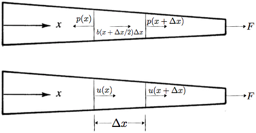
"## Axially Loaded Elastic Bar\n",
"\n",
"Consider the tapered bar\n",
"\n",
"
](#top)"
]
},
{
"cell_type": "markdown",
"metadata": {},
"source": [
" \n",
"## Axially Loaded Elastic Bar\n",
"\n",
"Consider the tapered bar\n",
"\n",
" \n",
"\n",
"Summing forces on the differential volumes gives\n",
"\n",
"$$-p(x) + b\\left(x+\\frac{\\Delta x}{2}\\right)\\Delta x + p\\left(x+\\Delta x\\right) = 0$$\n",
"\n",
"and taking the limit as $\\Delta x \\rightarrow 0$ leads to the following differential relationship \n",
"\n",
"$$\\lim_{\\Delta x \\rightarrow 0} \\frac{p\\left(x + \\Delta x\\right) -p\\left(x\\right)}{\\Delta x} + b\\left(x+\\frac{\\Delta x}{2}\\right) = \\frac{dp}{dx} + b(x) = 0$$\n",
"\n",
"Solution of the differential equation requires a *constitutive equation* relating $p(x)$ to $u(x)$. Recalling that\n",
"\n",
"$$\\sigma(x) = \\frac{p(x)}{A(x)} \\Rightarrow p(x) = \\sigma(x) A(x)$$\n",
"\n",
"and, for a simple linear elastic material, the stress $\\sigma$ is given by Hooke's law of linear elasticity†\n",
"\n",
"$$\\sigma(x)=E(x)\\epsilon(x)$$\n",
"\n",
"where the strain $\\epsilon$ is given by\n",
"\n",
"$$\\epsilon(x) = \\frac{\\Delta L}{L} = \\lim_{\\Delta x\\rightarrow 0} \\frac{u(\\Delta x) - u(x+\\Delta x)}{\\Delta x} = \\frac{du}{dx}$$\n",
"\n",
"Substituting the above expressions in to the differential relationship leads to\n",
"\n",
"$$\\frac{d}{dx}\\left(A(x)E(x)\\frac{du}{dx}\\right)+b(x)=0$$\n",
"\n",
"The above is a second-order ordinary differential equation. In the above equation, $u(x)$ is the dependent variable, which is the unknown function, and $x$ is the independent variable. \n",
"\n",
"To solve the strong form of the governing equation, boundary conditions at each end of the bar must be prescribed. For the purpose of illustration, we will consider the following specific boundary conditions: at $x=0$, the displacement, $u(x=0)$, is prescribed; at $x=L$, the force per unit area, or traction, denoted by $t$, is prescribed. These conditions are written as\n",
"\n",
"$$\n",
"\\begin{align}\n",
"u(x=0) &= \\overline{u} \\\\\n",
"\\sigma(x=L) &= \\left(E\\frac{du}{dx}\\right)_{x=L}=\\frac{F(L)}{A(L)} \\equiv \\overline{t} \n",
"\\end{align}\n",
"$$\n",
"\n",
"The traction $t$ has the same units as stress (force/area), but its sign is positive when it acts in the positive $x$-direction regardless of which face it is acting on, whereas the stress is positive in tension and negative in compression, so that on a negative face a positive stress corresponds to a negative traction.\n",
"\n",
"The differential equation governing the response of the elastic bar along with the associated boundary conditions is called the **strong form** of the governing equation and is summarized here\n",
"\n",
"
\n",
"\n",
"Summing forces on the differential volumes gives\n",
"\n",
"$$-p(x) + b\\left(x+\\frac{\\Delta x}{2}\\right)\\Delta x + p\\left(x+\\Delta x\\right) = 0$$\n",
"\n",
"and taking the limit as $\\Delta x \\rightarrow 0$ leads to the following differential relationship \n",
"\n",
"$$\\lim_{\\Delta x \\rightarrow 0} \\frac{p\\left(x + \\Delta x\\right) -p\\left(x\\right)}{\\Delta x} + b\\left(x+\\frac{\\Delta x}{2}\\right) = \\frac{dp}{dx} + b(x) = 0$$\n",
"\n",
"Solution of the differential equation requires a *constitutive equation* relating $p(x)$ to $u(x)$. Recalling that\n",
"\n",
"$$\\sigma(x) = \\frac{p(x)}{A(x)} \\Rightarrow p(x) = \\sigma(x) A(x)$$\n",
"\n",
"and, for a simple linear elastic material, the stress $\\sigma$ is given by Hooke's law of linear elasticity†\n",
"\n",
"$$\\sigma(x)=E(x)\\epsilon(x)$$\n",
"\n",
"where the strain $\\epsilon$ is given by\n",
"\n",
"$$\\epsilon(x) = \\frac{\\Delta L}{L} = \\lim_{\\Delta x\\rightarrow 0} \\frac{u(\\Delta x) - u(x+\\Delta x)}{\\Delta x} = \\frac{du}{dx}$$\n",
"\n",
"Substituting the above expressions in to the differential relationship leads to\n",
"\n",
"$$\\frac{d}{dx}\\left(A(x)E(x)\\frac{du}{dx}\\right)+b(x)=0$$\n",
"\n",
"The above is a second-order ordinary differential equation. In the above equation, $u(x)$ is the dependent variable, which is the unknown function, and $x$ is the independent variable. \n",
"\n",
"To solve the strong form of the governing equation, boundary conditions at each end of the bar must be prescribed. For the purpose of illustration, we will consider the following specific boundary conditions: at $x=0$, the displacement, $u(x=0)$, is prescribed; at $x=L$, the force per unit area, or traction, denoted by $t$, is prescribed. These conditions are written as\n",
"\n",
"$$\n",
"\\begin{align}\n",
"u(x=0) &= \\overline{u} \\\\\n",
"\\sigma(x=L) &= \\left(E\\frac{du}{dx}\\right)_{x=L}=\\frac{F(L)}{A(L)} \\equiv \\overline{t} \n",
"\\end{align}\n",
"$$\n",
"\n",
"The traction $t$ has the same units as stress (force/area), but its sign is positive when it acts in the positive $x$-direction regardless of which face it is acting on, whereas the stress is positive in tension and negative in compression, so that on a negative face a positive stress corresponds to a negative traction.\n",
"\n",
"The differential equation governing the response of the elastic bar along with the associated boundary conditions is called the **strong form** of the governing equation and is summarized here\n",
"\n",
"\n",
"
\n",
"\n",
"**Note**\n",
"- The problem data are $\\overline{u}$, $\\overline{t}$, and $b(x)$ and are given\n",
"- Either the load or the displacement can be specified at a boundary point, but not both.\n",
"\n",
"The strong form
\n", "$$\n", "\\begin{split}\n", "\\frac{d}{dx}\\left(A(x)E(x)\\frac{du}{dx}\\right)+b(x)=0 \\\\\n", "u(x=0) = \\overline{u} \\\\\n", "\\left(E\\frac{du}{dx}\\right)_{x=L} = \\overline{t} \n", "\\end{split}\n", "$$\n", "\n",
"†For thermo-elastic materials, the constitutive model is modified to include thermal effects $\\sigma(x) = E(x)\\left(\\epsilon(x) - \\alpha(x)T(x)\\right)$\n",
"
"
]
},
{
"cell_type": "markdown",
"metadata": {},
"source": [
"\n",
"
"
]
},
{
"cell_type": "markdown",
"metadata": {},
"source": [
" \n",
"## Heat Conduction\n",
"\n",
"Heat flow in a body occurs when there is a temperature difference within the body. Heat transferred in this way is referred to as conduction. The heat flow through the wall of a heated room in the winter is an example of conduction. In this section, the strong form of the differential equation governing heat transfer through conduction will be developed. Other forms of heat transfer such as convection will be discussed in later chapters.\n",
"\n",
"Remark
\n", "In the previous example there are two types of boundary conditions: one in which the dependent variable ($u$) was specified on the boundary and at the other boundary its derivative was $\\left(E du/dx\\right)$. These boundary conditions are classified as Dirichlet and Neummann, respectively.\n", "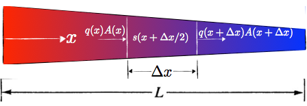 \n",
"\n",
"Consider a body as shown above. The objective is to determine the temperature distribution. Let $A(x)$ be the area normal to the direction of heat flow and let $s(x)$ be the heat generated per unit thickness of the body, denoted by l. This is often called a heat source. A common example of a heat source is the heat generated in an electric wire due to resistance. In the one-dimensional case, the rate of heat generation is measured in units of energy per time; in SI units, the units of energy are joules (J) per unit length (meters, m) and time (seconds, s). Recall that the unit of power is watts (1 W = 1 J/s). A heat source $s(x)$ is considered positive when heat is generated, i.e. added to the system, and negative when heat is withdrawn from the system. Heat flux, denoted by $q(x)$, is defined as a the rate of heat flow across a surface. Its units are heat rate per unit area; in SI units, W/m$^2$. It is positive when heat flows in the positive x-direction. We will consider a steady-state problem, i.e. a system that is not changing with time.\n",
"\n",
"To establish the differential equation that governs the system, we consider energy balance in a control volume of the wall. Energy balance requires that the rate of heat energy ($qA$) that is generated in the control volume must equal the heat energy leaving the control volume, as the temperature, and hence the energy in the control volume, is constant in a steady-state problem. The heat energy leaving the control volume is the difference between the flow in at on the left-hand side, $qA$, and the flow out on the right-hand side, $q(x + \\Delta x)A(x+\\Delta x)$. Thus, energy balance for the control volume can be written as\n",
"\n",
"$$s\\left(x+\\frac{\\Delta x}{2}\\right)\\Delta x + q(x)A(x) - q\\left(x+\\Delta x\\right)A(x+ \\Delta x) = 0$$\n",
"\n",
"Rearranging and taking the limit as $\\Delta x \\rightarrow 0$ leads to the following differential relationship \n",
"\n",
"$$\\lim_{\\Delta x \\rightarrow 0} \\frac{q\\left(x + \\Delta x\\right)A(x+\\Delta x) -q\\left(x\\right)A(x)}{\\Delta x} - s\\left(x+\\frac{\\Delta x}{2}\\right) = \\frac{d(qA)}{dx} - s = 0$$\n",
"\n",
"The constitutive equation for heat flow, which relates the heat flux to the temperature, is known as Fourier’s law and is given by\n",
"\n",
"$$\n",
"q = -k \\frac{dT}{dx}\n",
"$$\n",
"\n",
"where $T$ is the temperature and $k$ is the thermal conductivity (which must be positive); in SI units, the dimensions of thermal conductivity are W/m$\\cdot$oC. A negative sign appears because heat flows from high (hot) to low temperature (cold), i.e. opposite to the direction of the gradient of the temperature field. Substituting Fourier's law gives\n",
"\n",
"$$\\frac{d}{dx}\\left(Ak\\frac{dT}{dx}\\right) + s = 0, \\quad 0 < x < L$$\n",
"\n",
"Either the flux or the temperature must be prescribed on each end of the bar; these are the boundary conditions. We consider the specific boundary conditions of the prescribed temperature $\\overline{T}$ at $x=0$ and prescribed flux $\\overline{q}$ at $x=L$. The prescribed flux $\\overline{q}$ is positive if heat (energy) flows out of the bar, i.e. $q(x=L)=-\\overline{q}$. The strong form for the heat conduction problem is then given by\n",
"\n",
"
\n",
"\n",
"Consider a body as shown above. The objective is to determine the temperature distribution. Let $A(x)$ be the area normal to the direction of heat flow and let $s(x)$ be the heat generated per unit thickness of the body, denoted by l. This is often called a heat source. A common example of a heat source is the heat generated in an electric wire due to resistance. In the one-dimensional case, the rate of heat generation is measured in units of energy per time; in SI units, the units of energy are joules (J) per unit length (meters, m) and time (seconds, s). Recall that the unit of power is watts (1 W = 1 J/s). A heat source $s(x)$ is considered positive when heat is generated, i.e. added to the system, and negative when heat is withdrawn from the system. Heat flux, denoted by $q(x)$, is defined as a the rate of heat flow across a surface. Its units are heat rate per unit area; in SI units, W/m$^2$. It is positive when heat flows in the positive x-direction. We will consider a steady-state problem, i.e. a system that is not changing with time.\n",
"\n",
"To establish the differential equation that governs the system, we consider energy balance in a control volume of the wall. Energy balance requires that the rate of heat energy ($qA$) that is generated in the control volume must equal the heat energy leaving the control volume, as the temperature, and hence the energy in the control volume, is constant in a steady-state problem. The heat energy leaving the control volume is the difference between the flow in at on the left-hand side, $qA$, and the flow out on the right-hand side, $q(x + \\Delta x)A(x+\\Delta x)$. Thus, energy balance for the control volume can be written as\n",
"\n",
"$$s\\left(x+\\frac{\\Delta x}{2}\\right)\\Delta x + q(x)A(x) - q\\left(x+\\Delta x\\right)A(x+ \\Delta x) = 0$$\n",
"\n",
"Rearranging and taking the limit as $\\Delta x \\rightarrow 0$ leads to the following differential relationship \n",
"\n",
"$$\\lim_{\\Delta x \\rightarrow 0} \\frac{q\\left(x + \\Delta x\\right)A(x+\\Delta x) -q\\left(x\\right)A(x)}{\\Delta x} - s\\left(x+\\frac{\\Delta x}{2}\\right) = \\frac{d(qA)}{dx} - s = 0$$\n",
"\n",
"The constitutive equation for heat flow, which relates the heat flux to the temperature, is known as Fourier’s law and is given by\n",
"\n",
"$$\n",
"q = -k \\frac{dT}{dx}\n",
"$$\n",
"\n",
"where $T$ is the temperature and $k$ is the thermal conductivity (which must be positive); in SI units, the dimensions of thermal conductivity are W/m$\\cdot$oC. A negative sign appears because heat flows from high (hot) to low temperature (cold), i.e. opposite to the direction of the gradient of the temperature field. Substituting Fourier's law gives\n",
"\n",
"$$\\frac{d}{dx}\\left(Ak\\frac{dT}{dx}\\right) + s = 0, \\quad 0 < x < L$$\n",
"\n",
"Either the flux or the temperature must be prescribed on each end of the bar; these are the boundary conditions. We consider the specific boundary conditions of the prescribed temperature $\\overline{T}$ at $x=0$ and prescribed flux $\\overline{q}$ at $x=L$. The prescribed flux $\\overline{q}$ is positive if heat (energy) flows out of the bar, i.e. $q(x=L)=-\\overline{q}$. The strong form for the heat conduction problem is then given by\n",
"\n",
"\n",
"
"
]
},
{
"cell_type": "markdown",
"metadata": {},
"source": [
"## Electrical Conduction\n",
"\n",
"Consider the tapered bar with electrical potential as shown\n",
"\n",
"The strong form
\n", "$$\\begin{split}\n", "\\frac{d}{dx}\\left(Ak\\frac{dT}{dx}\\right) + s = 0, \\quad 0 < x < L \\\\\n", "T=\\overline{T} \\text{ on } x=0 \\\\\n", "-q=k\\frac{dT}{dx} = \\overline{q} \\text{ on } x=L\\\\\n", "\\end{split}\n", "$$\n", "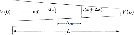 \n",
"\n",
"Conservation of charge requires that\n",
"\n",
"$$i(x) - i\\left(x+\\Delta x\\right) = 0$$\n",
"\n",
"rearranging and taking the limit as $\\Delta x \\rightarrow 0$ leads to the following differential relationship \n",
"\n",
"$$\\lim_{\\Delta x \\rightarrow 0} \\frac{i\\left(x\\right) -i\\left(x + \\Delta x\\right)}{\\Delta x} = -\\frac{di}{dx} = 0$$\n",
"\n",
"Ohm's law gives the constitutive equation relating voltagel and current \n",
"\n",
"$$\\begin{split}\n",
"V(x) - V(x+\\Delta x) = i \\frac{\\rho(\\Delta x)}{A\\left(x+\\frac{\\Delta x}{2}\\right)} \\\\\n",
"-\\frac{1}{\\rho}A(x)\\frac{dV}{dx} = i\n",
"\\end{split}$$\n",
"\n",
"where $\\rho$ is the resistivity. Substituting the above expressions in to the differential relationship leads to\n",
"\n",
"$$\\frac{d}{dx}\\left(\\frac{1}{\\rho}A(x)\\frac{dV}{dx}\\right)=0$$\n",
"\n",
"which is the strong from of the governing equation.\n",
"\n",
"Boundary conditions take the form of either a prescribed voltage or current at either end. The strong form for electrical conduction with voltage prescribed at $x=0$ and current prescribed at $x=L$ is given by\n",
"\n",
"
\n",
"\n",
"Conservation of charge requires that\n",
"\n",
"$$i(x) - i\\left(x+\\Delta x\\right) = 0$$\n",
"\n",
"rearranging and taking the limit as $\\Delta x \\rightarrow 0$ leads to the following differential relationship \n",
"\n",
"$$\\lim_{\\Delta x \\rightarrow 0} \\frac{i\\left(x\\right) -i\\left(x + \\Delta x\\right)}{\\Delta x} = -\\frac{di}{dx} = 0$$\n",
"\n",
"Ohm's law gives the constitutive equation relating voltagel and current \n",
"\n",
"$$\\begin{split}\n",
"V(x) - V(x+\\Delta x) = i \\frac{\\rho(\\Delta x)}{A\\left(x+\\frac{\\Delta x}{2}\\right)} \\\\\n",
"-\\frac{1}{\\rho}A(x)\\frac{dV}{dx} = i\n",
"\\end{split}$$\n",
"\n",
"where $\\rho$ is the resistivity. Substituting the above expressions in to the differential relationship leads to\n",
"\n",
"$$\\frac{d}{dx}\\left(\\frac{1}{\\rho}A(x)\\frac{dV}{dx}\\right)=0$$\n",
"\n",
"which is the strong from of the governing equation.\n",
"\n",
"Boundary conditions take the form of either a prescribed voltage or current at either end. The strong form for electrical conduction with voltage prescribed at $x=0$ and current prescribed at $x=L$ is given by\n",
"\n",
"\n",
"
\n",
"\n",
"The Strong Form
\n", "$$\n", "\\begin{split}\n", "\\frac{d}{dx}\\left(\\frac{1}{\\rho}A(x)\\frac{dV}{dx}\\right)=0 \\\\\n", "V(x=0) = \\overline{V} \\\\\n", "\\left(\\frac{1}{\\rho}A\\frac{dV}{dx}\\right)_{x=L} = \\overline{i} \n", "\\end{split}\n", "$$\n", "\n",
"
"
]
},
{
"cell_type": "markdown",
"metadata": {},
"source": [
" \n",
"# Flux Potential Relationships[Remark
\n", "To find the resistance of the entire element \n", "- \n",
"
- Prescribe a current BC $i(0) = \\overline{i} = 1A$ \n", "
- Prescribe a voltage BC $V(L) = 0$ \n", "
- Solve for V(0) \n", "
- Sove for resistance $R=\\frac{V(0) - V(L)}{i(0)} = \\frac{V(0)}{1 A}$ \n", "
](#top)\n",
"\n",
" \n",
"\n",
"## What is being fluxed?\n",
"\n",
"Flux is the rate of \"something\" per unit area. To determine what is being fluxed, multiply flux by area to identify the rate of the thing being fluxed\n",
"\n",
"### Heat\n",
"\n",
"The flux, $-qn$, has units W/m$^2$. Rate of the “thing” fluxed has units W.\n",
"A watt, W, has units of Joules/s. The thing fluxed has units of Joules.\n",
"\n",
"
\n",
"\n",
"## What is being fluxed?\n",
"\n",
"Flux is the rate of \"something\" per unit area. To determine what is being fluxed, multiply flux by area to identify the rate of the thing being fluxed\n",
"\n",
"### Heat\n",
"\n",
"The flux, $-qn$, has units W/m$^2$. Rate of the “thing” fluxed has units W.\n",
"A watt, W, has units of Joules/s. The thing fluxed has units of Joules.\n",
"\n",
" The thing fluxed is energy!
\n", "The heat equation is often called \"energy balance\"
\n", "Steady state: rate of energy is zero!
\n", "
\n",
"\n",
"### Elasticity\n",
"\n",
"The flux $\\bar{t}$ has units N/m$^2$. Rate of the “thing” fluxed has units N.\n",
"A Newton, N, has units kg m/s$^2$. The thing fluxed has units of kg m/s.\n",
"\n",
"\n", "The heat equation is often called \"energy balance\"
\n", "Steady state: rate of energy is zero!
\n", "
\n",
"That’s mass times velocity!
\n", "The thing fluxed is momentum!
\n", "The elasticity equation is often called “momentum balance”
\n", "Equilibrium: rate of momentum is zero!
\n", "
"
]
}
],
"metadata": {
"kernelspec": {
"display_name": "Python 2",
"language": "python",
"name": "python2"
},
"language_info": {
"codemirror_mode": {
"name": "ipython",
"version": 2
},
"file_extension": ".py",
"mimetype": "text/x-python",
"name": "python",
"nbconvert_exporter": "python",
"pygments_lexer": "ipython2",
"version": "2.7.10"
}
},
"nbformat": 4,
"nbformat_minor": 0
}
\n", "The thing fluxed is momentum!
\n", "The elasticity equation is often called “momentum balance”
\n", "Equilibrium: rate of momentum is zero!
\n", "