 \n",
"\n",
"
\n",
"\n",
" \n",
"\n",
"This lecture by Tim Fuller is licensed under the\n",
"Creative Commons Attribution 4.0 International License. All code examples are also licensed under the [MIT license](http://opensource.org/licenses/MIT)."
]
},
{
"cell_type": "markdown",
"metadata": {},
"source": [
"# Topics\n",
"- [Introduction](#intro)\n",
"- [Continuity](#continuity)\n",
"- [Weighted Integral Formulations](#weight-forms)\n",
" - [Three Steps to Develop the Weak Form](#three-steps)\n",
" - [Step 1](#step-1)\n",
" - [Step 2](#step-2)\n",
" - [Step 3](#step-3)\n",
"- [Summary](#summary)\n",
"- [Examples](#examples)\n",
" - [Example 1](#ex-1)\n",
" - [Example 2](#ex-2)"
]
},
{
"cell_type": "markdown",
"metadata": {},
"source": [
"# Introduction[
\n",
"\n",
"This lecture by Tim Fuller is licensed under the\n",
"Creative Commons Attribution 4.0 International License. All code examples are also licensed under the [MIT license](http://opensource.org/licenses/MIT)."
]
},
{
"cell_type": "markdown",
"metadata": {},
"source": [
"# Topics\n",
"- [Introduction](#intro)\n",
"- [Continuity](#continuity)\n",
"- [Weighted Integral Formulations](#weight-forms)\n",
" - [Three Steps to Develop the Weak Form](#three-steps)\n",
" - [Step 1](#step-1)\n",
" - [Step 2](#step-2)\n",
" - [Step 3](#step-3)\n",
"- [Summary](#summary)\n",
"- [Examples](#examples)\n",
" - [Example 1](#ex-1)\n",
" - [Example 2](#ex-2)"
]
},
{
"cell_type": "markdown",
"metadata": {},
"source": [
"# Introduction[ ](#top)\n",
"> The weak form is the most intellectually challenging part in the development of finite elements, so a student may encounter some difficulties in understanding this concept\n",
"\n",
"> Understanding how a solution to a differential equation can be obtained by this rather abstract statement, and why it is a useful solution, is not easy. It takes most students considerable thought and experience to comprehend the process.\n",
"\n",
"> - Fish and Belytschko, 2007\n",
"\n",
"The weighted integral formulations of the previous lesson allowed finding approximate solutions to the accompanying governing differential equation. Similarly, the finite element method is a technique for constructing approximate solutions to differential equations. To understand the foundations of the method, it is necessary to understand the weighted-integral formulations and the *weak* formulation of the differential equations. A weak form of a differential equation is equivalent to the governing equation and boundary conditions, i.e. the strong form. It allows classifying boundary conditions as essential and natural."
]
},
{
"cell_type": "markdown",
"metadata": {},
"source": [
"# Continuity[](#top)\n",
"\n",
"Before developing the weak form, let us discuss the concept of smoothness, or continuity. In general, a $k^{\\rm th}$ order ODE\n",
"\n",
"$$\n",
" au^{(k)} + a_{k-1}u^{(k-1)}+\\cdots++ a_{2}u''+ a_{1}u' + a_0=0\n",
"$$\n",
"\n",
"requires that\n",
"\n",
"$$\n",
" u\\in C^{k-1}\n",
"$$\n",
"\n",
"which means that $u$ has $k-1$ continuous derivatives. For example, if\n",
"\n",
"$$\n",
" \\frac{d^2u}{dx^2}=0\n",
"$$\n",
"\n",
"then $u\\in C^1$, or the first derivative of $u$ must be continuous. Let's see if this is true.\n",
"\n",
"$$\n",
" \\frac{d^2u}{dx^2} = 0 \\Rightarrow u=c_1x + c_2\n",
"$$\n",
"\n",
"and\n",
"\n",
"$$\n",
" u'=c_1\n",
"$$\n",
"\n",
"sure enough, $u'$ is continuous and $u\\in C^1$\n",
"\n",
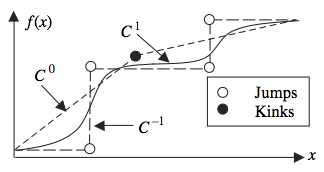
"A function is a $C^k$ function if its derivatives of order $j$ for $0 \\leq j \\leq k$ exist and are continuous functions in the entire domain. In finite element analysis, we are concerned mostly with $C^0$, $C^{-1}$ and $C^1$ functions\n",
"\n",
"
](#top)\n",
"> The weak form is the most intellectually challenging part in the development of finite elements, so a student may encounter some difficulties in understanding this concept\n",
"\n",
"> Understanding how a solution to a differential equation can be obtained by this rather abstract statement, and why it is a useful solution, is not easy. It takes most students considerable thought and experience to comprehend the process.\n",
"\n",
"> - Fish and Belytschko, 2007\n",
"\n",
"The weighted integral formulations of the previous lesson allowed finding approximate solutions to the accompanying governing differential equation. Similarly, the finite element method is a technique for constructing approximate solutions to differential equations. To understand the foundations of the method, it is necessary to understand the weighted-integral formulations and the *weak* formulation of the differential equations. A weak form of a differential equation is equivalent to the governing equation and boundary conditions, i.e. the strong form. It allows classifying boundary conditions as essential and natural."
]
},
{
"cell_type": "markdown",
"metadata": {},
"source": [
"# Continuity[](#top)\n",
"\n",
"Before developing the weak form, let us discuss the concept of smoothness, or continuity. In general, a $k^{\\rm th}$ order ODE\n",
"\n",
"$$\n",
" au^{(k)} + a_{k-1}u^{(k-1)}+\\cdots++ a_{2}u''+ a_{1}u' + a_0=0\n",
"$$\n",
"\n",
"requires that\n",
"\n",
"$$\n",
" u\\in C^{k-1}\n",
"$$\n",
"\n",
"which means that $u$ has $k-1$ continuous derivatives. For example, if\n",
"\n",
"$$\n",
" \\frac{d^2u}{dx^2}=0\n",
"$$\n",
"\n",
"then $u\\in C^1$, or the first derivative of $u$ must be continuous. Let's see if this is true.\n",
"\n",
"$$\n",
" \\frac{d^2u}{dx^2} = 0 \\Rightarrow u=c_1x + c_2\n",
"$$\n",
"\n",
"and\n",
"\n",
"$$\n",
" u'=c_1\n",
"$$\n",
"\n",
"sure enough, $u'$ is continuous and $u\\in C^1$\n",
"\n",
"A function is a $C^k$ function if its derivatives of order $j$ for $0 \\leq j \\leq k$ exist and are continuous functions in the entire domain. In finite element analysis, we are concerned mostly with $C^0$, $C^{-1}$ and $C^1$ functions\n",
"\n",
" \n",
"\n",
"As can be seen, a $C^0$ function is piecewise continuously differentiable, i.e. its first derivative is continuous except at selected points. The derivative of a $C^0$ function is a $C^{-1}$ function. So for example, if the displacement is a $C^0$ function, the strain is a $C^{-1}$ function. In general, the derivative of a $C^n$ function is $C^{n-1}$."
]
},
{
"cell_type": "markdown",
"metadata": {},
"source": [
"# Weighted-Integral and Weak Formulations[](#top)\n",
"\n",
"Consider the following differential equation\n",
"\n",
"$$\n",
"-\\frac{d}{dx}\\left(a(x)\\frac{du}{dx}\\right) = q(x) \\quad\n",
"\\text{for } 0 < x < L\n",
"$$\n",
"\n",
"The solution $u(x)$ is subject to the boundary conditions\n",
"\n",
"$$\n",
"u(0) = u_0, \\quad \\left.\\left(a\\frac{du}{dx}\\right)\\right|_{x=L}=Q_0\n",
"$$\n",
"\n",
"where $a$ and $q$ are known functions of $x$, $u_0$ and $Q_0$ are known values, and $L$ is the length of the domain. These are the problem data. The solution $u$ is the dependent variable of the problem. When $u_0\\neq0$ and/or $Q_0\\neq0$, the boundary conditions are nonhomogeneous and homogeneous otherwise.\n",
"\n",
"The sole purpose of developing the weighted-integral statement was to be able to obtain $N$ linearly independent algebraic relations among the coefficients of the approximation\n",
"\n",
"$$\n",
"u\\approx U_N = \\sum_{i=1}^N c_i\\phi_i(x) + \\phi_0(x)\n",
"$$\n",
"\n",
"## Three Steps to Form the Weak Form\n",
"\n",
"Reddy describes the following three steps to developing the weak form, if it exists, to a differnital equation:\n",
"\n",
"1. Multiply the equations by a weight function $w$ and integrate over the problem domain.\n",
"2. Distribute differentiation among the dependent variable and weight function.\n",
"3. Impose the boundary conditions."
]
},
{
"cell_type": "markdown",
"metadata": {},
"source": [
"### Step 1\n",
"\n",
"Move all expressions to one side, multiply by the weight function, and integrate over the domain\n",
"\n",
"$$\n",
"\\int_0^L w\\left(-\\frac{d}{dx}\\left(a\\frac{du}{dx}\\right)-q\\right)dx = 0, \\quad \\forall w\n",
"$$\n",
"\n",
"The expression in the outer parenthesis is not zero if $u$ is replaced by an approximation. Thus, the above expression is a statement that the error in the differential equation due to the approximation is zero in the weighted-integral sense.\n",
"\n",
"The weight function $w$ can be any nonzero, integrable function. The weighted-integral statement is equivalent only to the differential equation, and it does not include any boundary conditions.\n",
"\n",
"
\n",
"\n",
"As can be seen, a $C^0$ function is piecewise continuously differentiable, i.e. its first derivative is continuous except at selected points. The derivative of a $C^0$ function is a $C^{-1}$ function. So for example, if the displacement is a $C^0$ function, the strain is a $C^{-1}$ function. In general, the derivative of a $C^n$ function is $C^{n-1}$."
]
},
{
"cell_type": "markdown",
"metadata": {},
"source": [
"# Weighted-Integral and Weak Formulations[](#top)\n",
"\n",
"Consider the following differential equation\n",
"\n",
"$$\n",
"-\\frac{d}{dx}\\left(a(x)\\frac{du}{dx}\\right) = q(x) \\quad\n",
"\\text{for } 0 < x < L\n",
"$$\n",
"\n",
"The solution $u(x)$ is subject to the boundary conditions\n",
"\n",
"$$\n",
"u(0) = u_0, \\quad \\left.\\left(a\\frac{du}{dx}\\right)\\right|_{x=L}=Q_0\n",
"$$\n",
"\n",
"where $a$ and $q$ are known functions of $x$, $u_0$ and $Q_0$ are known values, and $L$ is the length of the domain. These are the problem data. The solution $u$ is the dependent variable of the problem. When $u_0\\neq0$ and/or $Q_0\\neq0$, the boundary conditions are nonhomogeneous and homogeneous otherwise.\n",
"\n",
"The sole purpose of developing the weighted-integral statement was to be able to obtain $N$ linearly independent algebraic relations among the coefficients of the approximation\n",
"\n",
"$$\n",
"u\\approx U_N = \\sum_{i=1}^N c_i\\phi_i(x) + \\phi_0(x)\n",
"$$\n",
"\n",
"## Three Steps to Form the Weak Form\n",
"\n",
"Reddy describes the following three steps to developing the weak form, if it exists, to a differnital equation:\n",
"\n",
"1. Multiply the equations by a weight function $w$ and integrate over the problem domain.\n",
"2. Distribute differentiation among the dependent variable and weight function.\n",
"3. Impose the boundary conditions."
]
},
{
"cell_type": "markdown",
"metadata": {},
"source": [
"### Step 1\n",
"\n",
"Move all expressions to one side, multiply by the weight function, and integrate over the domain\n",
"\n",
"$$\n",
"\\int_0^L w\\left(-\\frac{d}{dx}\\left(a\\frac{du}{dx}\\right)-q\\right)dx = 0, \\quad \\forall w\n",
"$$\n",
"\n",
"The expression in the outer parenthesis is not zero if $u$ is replaced by an approximation. Thus, the above expression is a statement that the error in the differential equation due to the approximation is zero in the weighted-integral sense.\n",
"\n",
"The weight function $w$ can be any nonzero, integrable function. The weighted-integral statement is equivalent only to the differential equation, and it does not include any boundary conditions.\n",
"\n",
"\n",
"The statement that the weighted integral equation must hold for all $w$ ($\\forall w$) is not arbitrary. If it were not for that statement, none of the following would hold true.\n",
"
"
]
},
{
"cell_type": "markdown",
"metadata": {},
"source": [
"### Step 2\n",
"\n",
"With the weighted-integral statement, $N$ algebraic relations among the $c_i$ for $N$ different choices of $w$ can be obtained. But, the approximation functions $\\phi_i$ must still be chosen such that $U_N$ is differentiable as many times as required by the original differential equation and satisfies the original boundary conditions. If the differentiation is distributed between the approximate solution $U_N$ and the weight function $w$, the resulting integral form will require weaker continuity on $\\phi_i$ and, hence, the weighted-integral statement is called the *weak form*.\n",
"\n",
"Starting with the integral statement, we integrate the first term in the expression by parts to obtain\n",
"\n",
"$$\n",
"\\begin{align}\n",
"0 &= \\int_0^L w\\left(-\\frac{d}{dx}\\left(a\\frac{du}{dx}\\right)-q\\right)dx \\\\\n",
"&= \\int_0^L w\\left(\\frac{dw}{dx}a\\frac{du}{dx}-wq\\right)dx - \\left[wa\\frac{du}{dx}\\right]_0^L\\\\\n",
"\\end{align}\n",
"$$\n",
"\n",
"\n",
"The integration by parts formula is given by\n",
"$$\n",
"\\int_0^L wdv = -\\int_0^Lvdw + \\left[wv\\right]_0^L\n",
"$$\n",
"
\n",
"\n",
"Note that the weight function is required to be differentiable at least once.\n",
"\n",
"From the above expression, we can identify two types of boundary conditions: *natural* and *essential*. The following rule is used to identify the natural boundary conditions: after completing Step 2, the coefficients of the weight function and its derivatives in the boundary expressions are called the *secondary variables*. Specification of the secondary variables on the boundary constitutes the *natural boundary conditions*. For this case, the coefficient of the weight function (the secondary variable) is $adu/dx$.\n",
"\n",
"The secondary variables always have a physical meaning. In the case of the axial bar problem, the secondary variable represents a traction $t$. The secondary variable will be denoted by\n",
"\n",
"$$\n",
"Q = \\left(a\\frac{du}{dx}\\right)n_x\n",
"$$\n",
"\n",
"where $n_x$ is the direction cosine:\n",
"\n",
"$$\n",
"\\begin{align}\n",
"n_x = &\\text{cosine of the angle between the } x \\\\\n",
" & \\text{ axis and the normal to the boundary}\n",
"\\end{align}\n",
"$$\n",
"\n",
"For 1D problems, $n_x=-1$ on the left end and $n_x=1$ at the right end of the domain.\n",
"\n",
"The dependent variable of the problem, expressed in the same form as the weight function appearing in the boundary term is called the *primary variable*. Its specification on the boundary consitutes the *essential boundary condition*. For our example, the dependent variable $u$ is the primary variable and the essential boundary condition is the specification of $u$ at the boundary points.\n",
"\n",
"\n",
"The number of primary and secondary variables is always the same, and each primary variable has an associated secondary variable (e.g., temperature and heat, displacement and force, etc.). Only one of the pair may be specified at a point on a boundary.\n",
"
\n",
"\n",
"In light of the above, a given problem can have boundary conditions in one of three categories:\n",
"\n",
"i) all boundary conditions are essential\n",
"ii) some of the boundary conditions are essential with the rest being natural\n",
"iii) all boundary conditions are natural\n",
"\n",
"With our notation, the weak form is written\n",
"\n",
"$$\n",
"0 = \\int_0^L\\left(a\\frac{dw}{dx}\\frac{du}{dx}-wq\\right)dx - (wQ)_0 - (wQ)_L\n",
"$$\n",
"\n",
"\"Weak\" refers to the reduced (weakened) continuity of $u$ which is now required only to be once differentiable, instead of twice. "
]
},
{
"cell_type": "markdown",
"metadata": {},
"source": [
"### Step 3\n",
"\n",
"We now impose the boundary conditions. We require that the weight function $w$ vanish at boundary points where the essential boundary conditions are specified. In other words, $w$ is required to satisfy the homogenous form of the specified essential boundary conditions of the problem. Why is this the case? In the weak formulation, the weight unction has the meaning of a *virtual* change of the primary variable. When the primary variable is prescribed at a point, the virtual change must be 0. For our example problem, the essential boundary condition is $u=u_0$; thus, the weight function $w$ is required to satisfy\n",
"\n",
"$$\n",
"w(0) = 0, \\quad \\text{because } u(0) = u_0\n",
"$$\n",
"\n",
"Since $w(0) = 0$ and\n",
"\n",
"$$\n",
"Q(L) = \\left(a\\frac{du}{dx}n_x\\right)\\Bigg|_{x=L}=\n",
"\\left(a\\frac{du}{dx}\\right)\\Bigg|_{x=L} = Q_0\n",
"$$\n",
"\n",
"our example problem reduces to\n",
"\n",
"$$\n",
"0 = \\int_0^L w\\left(a\\frac{dw}{dx}\\frac{du}{dx}-wq\\right)dx - w(L)Q_0\n",
"$$\n",
"\n",
"which is the weak form equivalent to the original differential equation with the associated natural boundary condition."
]
},
{
"cell_type": "markdown",
"metadata": {
"collapsed": true
},
"source": [
"# Summary[](#top)\n",
"\n",
"1. The weak form of a differential equation is a weighted integral statement that is equivalent to the strong form *and* the specified natural boundary conditions.\n",
"2. The weak form is developed by multiplying the differential equation by an arbitrary weight function, distributing differentiation among the primary variable and the weight function through integration by parts, and finally applying the boundary conditions.\n",
"3. After integrating by parts, the boundary terms are used to identify the forms of the primary and secondary variables.\n",
"4. Because of the restrictions placed on the weight function in the weak form, it must belong to the same space of functions as the approximation functions ($w \\sim \\phi_i$)."
]
},
{
"cell_type": "markdown",
"metadata": {},
"source": [
"# Examples[](#top)"
]
},
{
"cell_type": "markdown",
"metadata": {},
"source": [
"## Example 1\n",
"\n",
"Construct the weak and identify the primary and secondary variables for the nonlinear equation\n",
"\n",
"$$ \n",
"-\\frac{d}{dx}\\left(u\\frac{du}{dx}\\right) + f = 0 \\quad \\text{for} \\quad\n",
"0 < x < L\n",
"$$\n",
"$$\n",
"\\left(u\\frac{du}{dx}\\right)\\Bigg|_{x=0}=0, \\quad u(1)=\\sqrt{2}\n",
"$$\n",
"\n",
"### Solution\n",
"\n",
"Following the three step procedure, we write\n",
"\n",
"$$ \n",
"\\begin{align}\n",
"0 &= \\int_0^Lw\\left(-\\frac{d}{dx}\\left(u\\frac{du}{dx}\\right) + f\\right)dx\\\\\n",
"&=\\int_0^L\\left(u\\frac{dw}{dx}\\frac{du}{dx} \n",
"+ wf\\right)dx-\\left(w\\left(u\\frac{du}{dx}\\right)\\right)\\Bigg|_0^L\n",
"\\end{align}\n",
"$$\n",
"\n",
"Observation of the boundary term identifies $u$ as the primary variable and $u(du/dx)$ as the secondary variable.\n",
"\n",
"From the boundary conditions, since $w(1) = 0$ (why?) and $du/dx=0$ at $x=0$, we obtain for the weak form\n",
"\n",
"$$\n",
"0 = \\int_0^L \\left(u\\frac{dw}{dx}\\frac{du}{dx} + wf\\right)dx\n",
"$$\n",
"\n",
"\n",
"The weak form does not contain an expression that is linear in both $u$ and $v$."
]
},
{
"cell_type": "markdown",
"metadata": {},
"source": [
"## Example 2\n",
"\n",
"Construct the weak form and identify the primary and secondary variables of the following nonlinear differential equation\n",
"\n",
"$$\n",
"-\\frac{d}{dx}\\left(\\left(1 + 2x^2\\right)\\frac{du}{dx}\\right) + u = x^2\n",
"$$\n",
"$$\n",
"u(0) = 1, \\quad \\left(\\frac{du}{dx}\\right)_{x=1}=2\n",
"$$\n",
"\n",
"### Solution\n",
"\n",
"Following the three step procedure, we write\n",
"\n",
"$$\n",
"\\begin{align}\n",
"(1) \\quad & 0 = \\int_0^1w\\left(-\\frac{d}{dx}\\left(\\left(1 + 2x^2\\right)\\frac{du}{dx}\\right) + u - x^2\\right)dx\n",
"\\\\\n",
"(2) \\quad & 0 = \\int_0^1\\left(\\left(1 + 2x^2\\right)\\frac{dw}{dx}\\frac{du}{dx} + wu - wx^2\\right)dx - \\left(w\\left(1+2x^2\\right)\\frac{du}{dx}\\right)\\Bigg|_0^1\n",
"\\end{align}\n",
"$$\n",
"\n",
"From the boundary term, $u$ is the primary variable and $\\left(1+2x^2\\right)du/dx$ is the secondary variable. Since $du/dx=2$ at $x=1$ and $w=0$ at $x=0$, the weak form is\n",
"\n",
"$$\n",
"0 = \\int_0^1\\left(\\left(1 + 2x^2\\right)\\frac{dw}{dx}\\frac{du}{dx} + wu\\right)dx - \\int_0^1wx^2dx - 6w(1)\n",
"$$"
]
}
],
"metadata": {
"kernelspec": {
"display_name": "Python 2",
"language": "python",
"name": "python2"
},
"language_info": {
"codemirror_mode": {
"name": "ipython",
"version": 2
},
"file_extension": ".py",
"mimetype": "text/x-python",
"name": "python",
"nbconvert_exporter": "python",
"pygments_lexer": "ipython2",
"version": "2.7.10"
}
},
"nbformat": 4,
"nbformat_minor": 0
}