{
"cells": [
{
"cell_type": "code",
"execution_count": 1,
"metadata": {
"collapsed": false
},
"outputs": [
{
"data": {
"text/html": [
"\n"
],
"text/plain": [
""
]
},
"execution_count": 1,
"metadata": {},
"output_type": "execute_result"
}
],
"source": [
"import theme\n",
"theme.load_style()"
]
},
{
"cell_type": "markdown",
"metadata": {},
"source": [
"# Lesson 8: Derivation of FEM Equations in 1D\n",
"\n",
" \n",
"\n",
"
\n",
"\n",
" \n",
"\n",
"This lecture by Tim Fuller is licensed under the\n",
"Creative Commons Attribution 4.0 International License. All code examples are also licensed under the [MIT license](http://opensource.org/licenses/MIT)."
]
},
{
"cell_type": "markdown",
"metadata": {},
"source": [
"# Topics\n",
"\n",
"- [Steps to Derive the FE Equations](#intro)\n",
" - [Step 1: Describe the problem](#step-1)\n",
" - [Step 2: Discretize the problem domain](#step-2)\n",
" - [Step 3: Derive element equations](#step-3)\n",
" - [Step 4: Assemble blobal equations](#step-4) \n",
" - [Element Connectivity](#econn)\n",
" - [Examples](#examples)\n",
" - [Example 1: Linear element stiffness](#ex-1)\n",
" - [Example 2: Imposition of boundary conditions](#ex-2)\n",
" - [Example 3: Postprocessing](#ex-3)"
]
},
{
"cell_type": "markdown",
"metadata": {},
"source": [
"# Steps to Derive the FE Equations [
\n",
"\n",
"This lecture by Tim Fuller is licensed under the\n",
"Creative Commons Attribution 4.0 International License. All code examples are also licensed under the [MIT license](http://opensource.org/licenses/MIT)."
]
},
{
"cell_type": "markdown",
"metadata": {},
"source": [
"# Topics\n",
"\n",
"- [Steps to Derive the FE Equations](#intro)\n",
" - [Step 1: Describe the problem](#step-1)\n",
" - [Step 2: Discretize the problem domain](#step-2)\n",
" - [Step 3: Derive element equations](#step-3)\n",
" - [Step 4: Assemble blobal equations](#step-4) \n",
" - [Element Connectivity](#econn)\n",
" - [Examples](#examples)\n",
" - [Example 1: Linear element stiffness](#ex-1)\n",
" - [Example 2: Imposition of boundary conditions](#ex-2)\n",
" - [Example 3: Postprocessing](#ex-3)"
]
},
{
"cell_type": "markdown",
"metadata": {},
"source": [
"# Steps to Derive the FE Equations [ ](#top)\n",
"\n",
"We previously demonstrated how to use weighted residual methods to approximate the solutions to DE. Recall that, in each one of those methods our approximate solution was required to satisfy the boundary conditions of the problem. This becomes increasingly difficult as the problem geometry becomes more complex. In the finite element method, we divide the complex geometry into a collection of more simplified geometries called *finite elements*, so that we can construct approximate solutions over each element. We then combine the approximate solutions on each element to give a solution for the global problem. However, we require that the approximate solutions satisfy only the boundary conditions on their respective elements. Thus, the finite element method differs from the weighted residual methods because the approximation functions satisfy only the boundary conditions on a single element and not the whole domain.\n",
"\n",
"In this lesson, a derivation of the finite element equations for a 1D, 2${^{\\rm nd}}$ order ODE is presented. The following steps will be followed\n",
"\n",
"1. Describe and model the boundary value problem\n",
"2. Discretize the problem Domain\n",
"3. Derive element equations\n",
"4. Assemble element equations into global equations"
]
},
{
"cell_type": "markdown",
"metadata": {},
"source": [
"## Step 1: Describe and Model the Boundary Value Problem\n",
"\n",
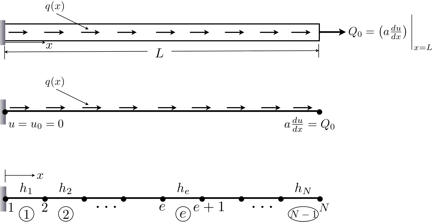
"Consider the problem of finding the function $u(x)$ that satisfies the following differential equation\n",
"\n",
"$$\n",
" \\frac{d}{dx}\\left(a(x) \\frac{du(x)}{dx}\\right) - c(x)u(x)+q(x) = 0 \\quad \\text{for } x \\in (0,L)\n",
"$$\n",
"\n",
"subject to the following boundary conditions\n",
"\n",
"$$\n",
" u(0)=u_0, \\quad \\left( a(x)\\frac{du(x)}{dx} \\right)\\Bigg|_{x=L}=Q_0\n",
"$$\n",
"\n",
"$a(x)$, $u(x)$, $c(x)$, and $q(x)$ are the known data of the problem. \n",
"\n",
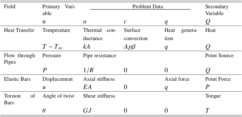
"Since $a(x)$, $u(x)$, $c(x)$, and $q(x)$ are all functions of $x$, we will write them as $a,$ $u,$ $c$, and $q$ for the remainder of the lesson. The boundary conditions are classified as essential ($u(0)=u_0$) and natural $\\left(\\left(adu/dx\\right)|_{x=L}=Q_0\\right)$. This is the **strong form** of the differential equation.\n",
"\n",
"This differential equation arises in many physical problems of interest to engineers, like heat transfer, flow through channels, transverse deflection of cables, and axial deformation of bars. The table below for a partial list of problems modeled by this equation. \n",
"\n",
"
](#top)\n",
"\n",
"We previously demonstrated how to use weighted residual methods to approximate the solutions to DE. Recall that, in each one of those methods our approximate solution was required to satisfy the boundary conditions of the problem. This becomes increasingly difficult as the problem geometry becomes more complex. In the finite element method, we divide the complex geometry into a collection of more simplified geometries called *finite elements*, so that we can construct approximate solutions over each element. We then combine the approximate solutions on each element to give a solution for the global problem. However, we require that the approximate solutions satisfy only the boundary conditions on their respective elements. Thus, the finite element method differs from the weighted residual methods because the approximation functions satisfy only the boundary conditions on a single element and not the whole domain.\n",
"\n",
"In this lesson, a derivation of the finite element equations for a 1D, 2${^{\\rm nd}}$ order ODE is presented. The following steps will be followed\n",
"\n",
"1. Describe and model the boundary value problem\n",
"2. Discretize the problem Domain\n",
"3. Derive element equations\n",
"4. Assemble element equations into global equations"
]
},
{
"cell_type": "markdown",
"metadata": {},
"source": [
"## Step 1: Describe and Model the Boundary Value Problem\n",
"\n",
"Consider the problem of finding the function $u(x)$ that satisfies the following differential equation\n",
"\n",
"$$\n",
" \\frac{d}{dx}\\left(a(x) \\frac{du(x)}{dx}\\right) - c(x)u(x)+q(x) = 0 \\quad \\text{for } x \\in (0,L)\n",
"$$\n",
"\n",
"subject to the following boundary conditions\n",
"\n",
"$$\n",
" u(0)=u_0, \\quad \\left( a(x)\\frac{du(x)}{dx} \\right)\\Bigg|_{x=L}=Q_0\n",
"$$\n",
"\n",
"$a(x)$, $u(x)$, $c(x)$, and $q(x)$ are the known data of the problem. \n",
"\n",
"Since $a(x)$, $u(x)$, $c(x)$, and $q(x)$ are all functions of $x$, we will write them as $a,$ $u,$ $c$, and $q$ for the remainder of the lesson. The boundary conditions are classified as essential ($u(0)=u_0$) and natural $\\left(\\left(adu/dx\\right)|_{x=L}=Q_0\\right)$. This is the **strong form** of the differential equation.\n",
"\n",
"This differential equation arises in many physical problems of interest to engineers, like heat transfer, flow through channels, transverse deflection of cables, and axial deformation of bars. The table below for a partial list of problems modeled by this equation. \n",
"\n",
" \n",
"\n",
"If a numerical solution to this differential equation is developed, taking into account all possible boundary conditions, the technique will be usable for each problem shown in the table. Thus, in this lesson the general $1D$ finite element equations are developed and over the next few days specific examples will be studied."
]
},
{
"cell_type": "markdown",
"metadata": {},
"source": [
"## Step 2: Discretize Problem Domain\n",
"\n",
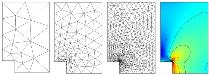
"The domain of the problem consists of all points between $x=0$ and $x=L$. Mathematically, we say $\\Omega=(0,L)$. We divide $\\Omega$ into a set of elements, as shown below. The collection of elements is called the finite element mesh.\n",
"\n",
"
\n",
"\n",
"If a numerical solution to this differential equation is developed, taking into account all possible boundary conditions, the technique will be usable for each problem shown in the table. Thus, in this lesson the general $1D$ finite element equations are developed and over the next few days specific examples will be studied."
]
},
{
"cell_type": "markdown",
"metadata": {},
"source": [
"## Step 2: Discretize Problem Domain\n",
"\n",
"The domain of the problem consists of all points between $x=0$ and $x=L$. Mathematically, we say $\\Omega=(0,L)$. We divide $\\Omega$ into a set of elements, as shown below. The collection of elements is called the finite element mesh.\n",
"\n",
" \n",
"\n",
"With the finite element method, an approximate solution to the equations governing some physical process on each element is sought. Then, the approximate global solution over the whole domain is determined by assembling element contributions.\n",
"\n",
"As in the direct method, the endpoints of each element are identified as the element nodes. The solution to the differential equation is required to be continuous at each node. As will be shown, the element nodes play the role of interpolation points in constructing the approximate solution over an element."
]
},
{
"cell_type": "markdown",
"metadata": {},
"source": [
"## Step 3: Derive Element Equations\n",
"\n",
"The finite element equations for the $e^{\\rm th}$ element, $\\Omega^{(e)}$, will now be derived\n",
"\n",
"
\n",
"\n",
"With the finite element method, an approximate solution to the equations governing some physical process on each element is sought. Then, the approximate global solution over the whole domain is determined by assembling element contributions.\n",
"\n",
"As in the direct method, the endpoints of each element are identified as the element nodes. The solution to the differential equation is required to be continuous at each node. As will be shown, the element nodes play the role of interpolation points in constructing the approximate solution over an element."
]
},
{
"cell_type": "markdown",
"metadata": {},
"source": [
"## Step 3: Derive Element Equations\n",
"\n",
"The finite element equations for the $e^{\\rm th}$ element, $\\Omega^{(e)}$, will now be derived\n",
"\n",
" \n",
"\n",
"The derivation of the finite element equations, i.e., the set of algebraic equations which relate the value of the primary variable to the secondary variables at the nodes, will be done using the following steps:\n",
"\n",
"**a)** Construct the weak form of the governing differential equation\n",
"\n",
"**b)** Assume the form of the approximate solution over a typical element \n",
"\n",
"**c)** Derive the FE equations by substituting the assumed form of the solution into the weak form of the governing DE \n",
"\n",
"### a) Construct the weak form of the governing differential equation\n",
"\n",
"The governing differential equation and associated boundary conditions is called the ''strong form'' of the governing equations. The ''weak'' form of the governing differential equation lends itself more easily to the finite element method. The motivation for doing this will be discussed after deriving the weak form.\n",
"\n",
"Recall the strong form of the governing differential equation:\n",
"\n",
"$$ \\frac{d}{dx}\\left( a\\frac{du}{dx}\\right) -cu+ q = 0 $$\n",
"\n",
"The weak form is derived following the three step process in [Lesson 7](Lesson7_TheWeakForm.ipynb). Namely, we first multiply the differential equation by a weight function and integrate over the problem domain\n",
"\n",
"$$ \n",
"\\int_{0}^{L}\\left( \\frac{d}{dx}\\left( a\\frac{du}{dx}\\right) -cu+ q \\right) w(x) dx=0 \n",
"$$\n",
"\n",
"Since $w(x)$ is a function of only $x$ we will write it simply as $w$. Recall that we can write this integral as\n",
"\n",
"$$\n",
" \\int_{0}^{L}\\left( \\frac{d}{dx}\\left( a\\frac{du}{dx}\\right) -cu+ q \\right) w dx= \\sum_e\\int_{\\Omega_e}\\left( \\frac{d}{dx}\\left( a\\frac{du}{dx}\\right) -cu+ q \\right) w dx=0\n",
"$$\n",
"\n",
"where $\\Omega_e=[x_1^{(e)}, x_2^{(e)}]$ is an individual element domain. Concentrating only on the $e^{\\text{th}}$ element, we have\n",
"\n",
"$$\n",
" \\int_{x_1^{(e)}}^{x_2^{(e)}} \\left( \\frac{d}{dx}\\left( a\\frac{du}{dx}\\right) w -cwu+ qw \\right)dx=0\n",
"$$\n",
"\n",
"Integrating the above expression by parts to transfer a derivative from $u$ to $w$, gives\n",
"\n",
"$$\n",
" = \\int_{x_1^{(e)}}^{x_2^{(e)}} \\frac{d}{dx}\\left( aw\\frac{du}{dx}\\right)dx - \\int_{x_1^{(e)}}^{x_2^{(e)}} a\\frac{du}{dx}\\frac{dw}{dx}dx + \\int_{x_1^{(e)}}^{x_2^{(e)}}\\left( qw -cwu \\right)dx =0\n",
"$$\n",
"\n",
"$$\n",
" \\left( aw\\frac{du}{dx} \\right) \\Bigg|_{x_1^{(e)}}^{x_2^{(e)}} - \\int_{x_1^{(e)}}^{x_2^{(e)}}{ a\\frac{du}{dx}\\frac{dw}{dx}dx} + \\int_{x_1^{(e)}}^{x_2^{(e)}}\\left( qw-cwu \\right) \\,\\mathrm{d}{x} =0\n",
"$$\n",
"\n",
"re-arranging\n",
"\n",
"$$\n",
" \\int_{x_1^{(e)}}^{x_2^{(e)}}\\left( a\\frac{du}{dx}\\frac{dw}{dx}+cwu-qw \\right)dx - wa\\frac{du}{dx}\\Bigg|_{x_1^{(e)}}^{x_2^{(e)}} =0 \n",
"$$\n",
"\n",
"Note that the essential and natural boundary conditions of the strong from arise naturally in the weak formulation. The classification of essential and natural boundary conditions is an important part of the variational formulation of the governing DE, thus we spend a moment going over the rules of their classification.\n",
"After trading differentiation between the weight function and the dependent variable, examine all boundary terms of the integral statement. The boundary terms will always involve both the weight function and the dependent variable. Coefficients of the weight function and its derivatives in the boundary expressions are termed the *secondary variables* and their specification on the boundary constitutes the *natural boundary conditions*. For our case, the boundary term $w(adu/dx)$ tells us that $adu/dx$ is the secondary variable and its specification on the boundary is the natural boundary condition.\n",
"The secondary variables always have physical meaning. In the case of heat transfer problems, the secondary variable represents heat, $Q$. We shall denote the secondary variable by\n",
"\n",
"\n",
"$$\n",
" Q=\\left( a \\frac{du}{dx} \\right) n_x\n",
"$$\n",
"\n",
"\n",
"where $n_x$ denotes the direction cosine, i.e., the angle between the $x$ axis and the normal to the boundary. For one dimensional problems, the normal is always along the length of the domain. Thus, $n_x=-1$ at the left end and $n_x=1$ at the right end of the domain.\n",
"The dependent variable of the problem, expressed in the same form as the weight function appearing in the boundary term, is called the *primary variable* and its specification on the boundary constitutes the *essential boundary conditions*. For the case in consideration, the weight function appears in the boundary expression as $w$. Therefore, the dependent variable $u$ is the primary variable and the essential boundary condition involves specifying $u$ at the boundary points.\n",
"\n",
"It should be noted that the number and form of the primary and secondary variables depend on the order of the differential equation. The number of primary and secondary variables is always the same and with each primary variable there is an associated secondary variable. For example - force and displacement, and heat and temperature. Only one of the pair, either the primary or the seondary variable, may be specified at a point of the boundary. Thus, a given problem can have its specified boundary conditions in one of three categories:\n",
"\n",
"\n",
"- All specified boundary conditions are essential (Dirichlet boundary conditions)\n",
"- Specified boundary conditions contain both essential and natural boundary conditions (mixed boundary conditions)\n",
"- All specified boundary conditions are natural (Von Neumann boundary conditions)\n",
"\n",
"\n",
"In general, a $2m^{\\rm th}$-order DE has $m$ primary variables and $m$ secondary variables.\n",
"In general, because $w$ is required to satisfy the boundary conditions of the problem the specification of $w$ and any of its derivatives constitute the essential boundary conditions. Likewise, the coefficients of $w$ or any of its derivatives constitute the natural boundary conditions.\n",
"If we now assume that all boundary conditions at the element level are of the natural type, we can re-write the term on the right hand side as\n",
"\n",
"\n",
"$$\n",
" aw\\frac{du}{dx}\\Bigg|_{x_1^{(e)}}^{x_2^{(e)}} = w(x_2^{(e)})Q_{{e+1}} + w(x_{e})Q_{{e}}\n",
"$$\n",
"\n",
"\n",
"and finally,\n",
"\n",
"\n",
"$$\n",
" \\int_{x_1^{(e)}}^{x_2^{(e)}} \\left( a\\frac{du}{dx}\\frac{dw}{dx}+cwu-wq\\right)dx - w(x_1^{(e)})Q_{{e}} - w(x_2^{(e)})Q_{{e+1}} =0\n",
"$$\n",
"\n",
"which is the weak form of the differential equation on element $e$. \n",
"\n",
"Recall that in the strong form the solution $u\\in C^1$ but in the weak form, because differentiation was transferred from $u$ to $w$, the continuity requirements were weakend so that now $u\\in C^0$. Weak and strong have nothing to do with the physical stature of the equation, only the continuity requirements on the solution.\n",
"\n",
"### b) Assume the form of the approximate solution over a typical element\n",
"\n",
"Note that the weak form over an element is equivalent to the differential equation and the natural boundary conditions on the element. However, the essential boundary conditions, $u(x_1^{(e)})=u_1^{(e)}$ and $u(x_2^{(e)})=u_2^{(e)}$, are not included in the weak form. Hence, as per our discussion of weighted residual methods, the approximation of $u$ must satisfy the essential boundary condtions. In other words, if $U_N^{(e)}$ is an approximation to $u$ on $\\Omega_{e}$ than it must be an interpolant between the nodes of the element, i.e., it must be equal to $u_1$ at $x_1^{(e)}$ and $u_2$ at $x_2^{(e)}$.\n",
"\n",
"We will now **assume** an approximate solution $U_N^{(e)}$ in the form of algebraic polynomials. We choose polynomials for two reasons - first, polynomials that satisfy the essential boundary conditions are easy to find over an element; second, integration of algebraic polynomials is easy. As in the weighted residual methods, the approximate solution must satisfy the following requirements:\n",
"\n",
"- The approximate solution should be continuous over the element and differentiable, as required by the weak form\n",
"- It must form a \"complete basis\" for the function space from which it is chosen\n",
"- It should be an interpolant of the primary variables at the nodes of the finite element\n",
"\n",
"The first requirement ensures a nonzero coefficient matrix and the third requirement is necessary in order to satisfy the essential boundary conditions of the element and to enforce continuity of the primary variables at points common to several elements. Let us now turn our attention to the second requirement. The second requirement is necessary to capture all possible states, i.e., constant, linear, and so on, of the actual solution. An approximation function forms a complete basis if it is capable of converging to any continuous function as terms are added. For example, the displacement function\n",
"\n",
"\n",
"$$\n",
" \\psi = c_0 + c_1 x + \\cdots + c_nx^n\n",
"$$\n",
"\n",
"\n",
"is complete because as $k\\rightarrow\\infty$ $u$ becomes a Taylor series which is capable of converging on any (well behaved) function. However, the displacement function\n",
"\n",
"\n",
"$$\n",
" \\psi = c_0 + c_4x^4 + \\cdots + c_nx^n\n",
"$$\n",
"\n",
"\n",
"is not a complete basis because it is missing the $c_1x, \\ c_2x^2,$ and $c_3x^3$ terms.\n",
"For the weak form of the governing equation, the minimum polynomial order required of the approximate solution is linear. Thus, a complete linear polynomial will have the form:\n",
"\n",
"\n",
"$$\n",
" ^{(e)}=a_1 + a_2x, \\ \\ \\ \\ a_1,a_2\\in{\\rm I\\kern-.16em R}\n",
"$$\n",
"\n",
"Note that this satisfies the first two requirements. Also note that there are two unknown coefficients $a_1,a_2$. We find the unknown coefficients by demanding that our approximate solution satisfies the third requirement:\n",
"\n",
"\n",
"$$\n",
" U_N^{(e)}(x_1^{(e)})=u_1^{(e)}, \\ \\ \\ \\ U_N^{(e)}(x_2^{(e)})=u_{2}^{(e)}\n",
"$$\n",
"\n",
"this now gives a relationship between the constants $a_1,a_2$ and the displacements $u_1^{(e)},u_{2}^{(e)}$\n",
"\n",
"\n",
"$$\n",
" U_N^{(e)}(x_1^{(e)})=u_1^{(e)}=a_1+a_2x_1^{(e)}\n",
"$$\n",
"\n",
"\n",
"\n",
"\n",
"$$\n",
" U_N^{(e)}(x_2^{(e)})=u_{2}^{(e)}=a_1+a_2x_2^{(e)}\n",
"$$\n",
"\n",
"\n",
"or, in matrix form\n",
"\n",
"\n",
"$$\n",
" \\left\\{ \\begin{array}{c} u_1^{(e)} \\\\ u_{2}^{(e)} \\end{array} \\right\\} = \\left[\\begin{array}{cc} 1 & x_1^{(e)} \\\\ 1 & x_2^{(e)} \\end{array} \\right] \\left\\{ \\begin{array}{c} a_1 \\\\ a_2 \\end{array} \\right\\}\n",
"$$\n",
"\n",
"\n",
"Solving for $a_1$ and $a_2$ gives\n",
"\n",
"\n",
"$$\n",
" a_1= \\frac{u_1^{(e)}x_2^{(e)}-u_{2}^{(e)}x_1^{(e)}}{x_2^{(e)}-x_1^{(e)}}\n",
"$$\n",
"\n",
"\n",
"\n",
"\n",
"$$\n",
" a_2=\\frac{u_{2}^{(e)}-u_1^{(e)}}{x_2^{(e)}-x_1^{(e)}}\n",
"$$\n",
"\n",
"\n",
"and\n",
"\n",
"\n",
"$$\n",
" U_N^{(e)} = \\frac{u_1^{(e)}x_2^{(e)}-u_{2}^{(e)}x_1^{(e)}}{x_2^{(e)}-x_1^{(e)}} + \\frac{u_{2}^{(e)}-u_1^{(e)}}{x_2^{(e)}-x_1^{(e)}}x\n",
"$$\n",
"\n",
"\n",
"after some re-arranging, the approximate solution can be written\n",
"\n",
"\n",
"$$\n",
" U_N^{(e)} = N_1^{(e)} u_1^{(e)} + N_{2}^{(e)} u_{2}^{(e)}\n",
"$$\n",
"\n",
"where\n",
"\n",
"\n",
"$$\n",
" N_1^{(e)}(x) = \\frac{x_2^{(e)}-x}{h_e}, \\qquad\n",
" N_{2}^{(e)}(x) = \\frac{x-x_1^{(e)}}{h_e}\n",
"$$\n",
"\n",
"and\n",
"\n",
"\n",
"$$\n",
" h_e = x_2^{(e)}-x_1^{(e)}\n",
"$$\n",
"\n",
"\n",
"is the length of the element. These equations are the general linear finite element approximation functions. Note that these equations are the Lagrange interpolation functions for the nodes of the elements.\n",
"\n",
"We further simplify the notation by noting that the element interpolation functions $N_i^{(e)}$ are expressed in terms of the *global coordinates* $x$ (i.e., the coordinate of the problem), but they are defined only on the element domain $\\Omega^{(e)}=(x_1^{(e)},x_2^{(e)})$. If we choose to express them in terms of a coordinate $\\hat{x}$ with origin fixed at node 1 of the element, the $N_i^{(e)}$ take the following forms\n",
"\n",
"$$ N_1^{(e)}(x)\\Rightarrow N_1^{(e)}(\\hat{x}) =\\frac{x_2-\\hat{x}}{h_e}=1-\\frac{\\hat{x}}{h_e} $$\n",
"$$ N_{2}^{(e)}(x)\\Rightarrow N_2^{(e)}(\\hat{x})=\\frac{\\hat{x}-x_1}{h_e}=\\frac{\\hat{x}}{h_e} $$\n",
"\n",
"We call the coordinate $\\hat{x}$ the *local* or *element coordinate*. Note that $N_1^{(e)}$ is equal to one at node one and zero at node two and $N_2^{(e)}$ is equal to zero at node one and one at node two. In other words, $N_i^{(e)}$ are interpolation functions of $u$. This property can be written as\n",
"\n",
"\n",
"\n",
"$$\n",
" N_i^{(e)}(x_j) = \\left\\{ \\begin{array}{c} 1 \\ \\ {\\rm if} \\ i=j \\\\ 0 \\ \\ {\\rm if} \\ i\\neq j \\end{array} \\right.\n",
"$$\n",
"\n",
"Using the local form of the interpolation functions, the approximate solution $U_N^{(e)}$ is written\n",
"\n",
"\n",
"$$\n",
" U_N^{(e)}=\\left[ \\begin{array}{cc}N_1^{(e)} & N_2^{(e)} \\end{array} \\right] \\left\\{ \\begin{array}{c} u_1^{(e)} \\\\[8pt] u_2^{(e)} \\end{array} \\right\\}\n",
"$$\n",
"\n",
"or, in a more compact form, we write\n",
"\n",
"\n",
"$$\n",
" U_N^{(e)}=\\sum_{j=1}^2 u_j^{(e)}N_j^{(e)}\n",
"$$\n",
"\n",
"\n",
"\n",
"## c) The Finite Element Model\n",
"\n",
"The weak form is equivalent to the governing differential equation over the element $\\Omega^{(e)}$ and also contains the natural boundary conditions. Further, the finite element approximation satisfies the essential boundary conditions of the element. Choosing a sufficient number of weight functions gives the necessary algebraic equations to determine the nodal values $u_i^{(e)}$ and $Q_i^{(e)}$ of the element $\\Omega^{(e)}$.\n",
"\n",
"Following the Galerkin method, we choose\n",
"\n",
"$$\n",
"w = \\sum_{i=1}^2w_i^{(e)}N_i^{(e)}\n",
"$$\n",
"\n",
"After substitution\n",
"\n",
"$$\n",
" \\int_{x_1^{(e)}}^{x_2^{(e)}}\\left( a\\frac{d\\left({\\sum_{i=1}^{2}w_i^{(e)}N_i^{(e)}}\\right)}{dx}\\frac{d\\left( {\\sum_{j=1}^{2}u_j^{(e)}N_j^{(e)}}\\right)}{dx}+ c\\sum_{i=1}^{2}w_i^{(e)}N_i^{(e)}\\sum_{j=1}^{2}u_j^{(e)}N_j^{(e)}- q\\sum_{i=1}^{2}w_i^{(e)}N_i^{(e)} \\right) \\,\\mathrm{d}{x}\n",
" - \\sum_{i=1}^{2}w_i^{(e)}N_i^{(e)}(x_1^{(e)})Q_1^{(e)}-\\sum_{i=1}^{2}w_i^{(e)}N_i^{(e)}(x_2^{(e)})Q_2^{(e)}=0\n",
"$$\n",
"\n",
"$$\n",
" =\\int_{x_1^{(e)}}^{x_2^{(e)}} \\left( a\\sum_{i=1}^2w_i^{(e)}\\sum_{j=1}^2u_j^{(e)}\\frac{dN_i^{(e)}}{dx}\\frac{dN_j^{(e)}}{dx}+ c\\sum_{i=1}^{2}w_i^{(e)}N_i^{(e)}\\sum_{j=1}^{2}u_j^{(e)}N_j^{(e)}- q\\sum_{i=1}^2w_i^{(e)}N_i^{(e)} \\right)\\,\\mathrm{d}{x}\n",
" - \\sum_{i=1}^{2}w_i^{(e)}\\left( N_i^{(e)}(x_1^{(e)})Q_1^{(e)} + N_i^{(e)}(x_2^{(e)})Q_2^{(e)} \\right)=0\n",
"$$\n",
"\n",
"$$\n",
" =\\sum_{i=1}^2w_i^{(e)}\\left[ \\int_{x_1^{(e)}}^{x_2^{(e)}}\\left( a\\sum_{j=1}^2u_j^{(e)}\\frac{dN_i^{(e)}}{dx}\\frac{dN_j^{(e)}}{dx}+cN_i^{(e)}\\sum_{j=1}^{2}u_j^{(e)}N_j^{(e)} - qN_i^{(e)} \\right)\\,\\mathrm{d}{x} - N_i^{(e)}(x_1^{(e)})Q_1^{(e)} -N_i^{(e)}(x_2^{(e)})Q_2^{(e)}\\right] =0\n",
"$$\n",
"\n",
"$$\n",
" =\\int_{x_1^{(e)}}^{x_2^{(e)}}\\left( a \\sum_{j=1}^2u_j^{(e)}\\frac{dN_i^{(e)}}{dx}\\frac{dN_j^{(e)}}{dx}+cN_i^{(e)}\\sum_{j=1}^{2}u_j^{(e)}N_j^{(e)} - qN_i^{(e)} \\right)\\,\\mathrm{d}{x}- N_i^{(e)}(x_1^{(e)})Q_1^{(e)} -N_i^{(e)}(x_2^{(e)})Q_2^{(e)} =0\n",
"$$\n",
"\n",
"Re-arranging\n",
"\n",
"$$\n",
" \\sum_{j=1}^2u_j^{(e)}\\int_{x_1^{(e)}}^{x_2^{(e)}}\\left( a \\frac{dN_i^{(e)}}{dx}\\frac{dN_j^{(e)}}{dx}+cN_i^{(e)}N_j^{(e)}\\right)\\,\\mathrm{d}{x} = \\int_{x_1^{(e)}}^{x_2^{(e)}} qN_i^{(e)} \\,\\mathrm{d}{x} \\ +\\ N_i^{(e)}(x_1^{(e)})Q_1^{(e)} +N_i^{(e)}(x_2^{(e)})Q_2^{(e)}\n",
"$$\n",
"\n",
"It is hard to see, but this is a set of 2 equations (1 equation for each free index $i$) for the two unknowns $u_1^{(e)}$ and $u_2^{(e)}$. Let's expand to see explicitly:\n",
"\n",
"$$\n",
" i=1\\Rightarrow \\sum_{j=1}^2u_j^{(e)}\\int_{x_1^{(e)}}^{x_2^{(e)}}\\left( a \\frac{dN_j^{(e)}}{dx}\\frac{dN_1^{(e)}}{dx}+cN_1^{(e)}N_j^{(e)}\\right)\\,\\mathrm{d}{x} = \\int_{x_1^{(e)}}^{x_2^{(e)}} qN_1^{(e)} \\,\\mathrm{d}{x} \\ +\\ N_1^{(e)}(x_1^{(e)})Q_1^{(e)} +N_1^{(e)}(x_2^{(e)})Q_2^{(e)}\n",
"$$\n",
"\n",
"$$\n",
" i=2\\Rightarrow \\sum_{j=1}^2u_j^{(e)}\\int_{x_1^{(e)}}^{x_2^{(e)}}\\left( a \\frac{dN_j^{(e)}}{dx}\\frac{dN_2^{(e)}}{dx}+cN_2^{(e)}N_j^{(e)}\\right)\\,\\mathrm{d}{x} = \\int_{x_1^{(e)}}^{x_2^{(e)}} qN_2^{(e)} \\,\\mathrm{d}{x} \\ +\\ N_2^{(e)}(x_1^{(e)})Q_1^{(e)} +N_2^{(e)}(x_2^{(e)})Q_2^{(e)}\n",
"$$\n",
"\n",
"These equations can now be written as\n",
"\n",
"$$\n",
" \\sum_{j=1}^2u_j^{(e)}\\int_{x_1^{(e)}}^{x_2^{(e)}}\\left( a \\frac{dN_j^{(e)}}{dx}\\frac{dN_1^{(e)}}{dx}+cN_1^{(e)}N_j^{(e)}\\right)\\,\\mathrm{d}{x} = \\int_{x_1^{(e)}}^{x_2^{(e)}} qN_1^{(e)} \\,\\mathrm{d}{x} \\ +\\ Q_1^{(e)}\n",
"$$\n",
"\n",
"$$\n",
" \\sum_{j=1}^2u_j^{(e)}\\int_{x_1^{(e)}}^{x_2^{(e)}}\\left( a \\frac{dN_j^{(e)}}{dx}\\frac{dN_2^{(e)}}{dx}+cN_2^{(e)}N_j^{(e)}\\right)\\,\\mathrm{d}{x} = \\int_{x_1^{(e)}}^{x_2^{(e)}} qN_2^{(e)} \\,\\mathrm{d}{x} \\ +\\ Q_2^{(e)}\n",
"$$\n",
"\n",
"\n",
"Which emits the following compact form of the finite element equations\n",
"\n",
"$$\n",
" k^{(e)}_{ij}u_j^{(e)} = f_i^{(e)} + Q_i^{(e)}\n",
"$$\n",
"\n",
"where\n",
"\n",
"$$\n",
" k^{(e)}_{ij}=\\int_{x_1^{(e)}}^{x_2^{(e)}} \\left( a\\frac{dN_i^{(e)}}{dx}\\frac{dN_j^{(e)}}{dx} + cN_i^{(e)}N_j^{(e)}\\right) \\,\\mathrm{d}{x}\n",
"$$\n",
"\n",
"and\n",
"\n",
"$$\n",
" f_i^{(e)}=\\int_{x_1^{(e)}}^{x_2^{(e)}} qN_i^{(e)} \\,\\mathrm{d}{x}\n",
"$$\n",
"\n",
"Recall that the $u_j$ are the unknown coefficients of our approximate solution. In matrix notation we write\n",
"\n",
"$$\n",
" [k^{(e)}]\\{u^{(e)}\\}=\\{f^{(e)}\\} + \\{Q^{(e)}\\}\n",
"$$\n",
"\n",
"\n",
"and in direct notation\n",
"\n",
"$$\n",
" {\\boldsymbol{k}}^{(e)}{\\boldsymbol{u}}^{(e)}={\\boldsymbol{f}}^{(e)} + {\\boldsymbol{Q}}^{(e)}\n",
"$$"
]
},
{
"cell_type": "markdown",
"metadata": {},
"source": [
"## Assemble Global Equations\n",
"\n",
"The global equations are assembled as\n",
"\n",
"\n",
"$$\n",
" \\int_{0}^{L}\\left( \\frac{d}{dx}\\left( a\\frac{du}{dx}\\right) -cu+ q \\right) w \\,\\mathrm{d}{x}= \\sum_e\\int_{\\Omega_e}\\left( \\frac{d}{dx}\\left( a\\frac{du}{dx}\\right) -cu+ q \\right) w dx=0\n",
"$$\n",
"\n",
"$$\n",
" \\sum_e k^{(e)}_{ij}u_j^{(e)} = \\sum_e \\left( f_i^{(e)} + Q_i^{(e)}\\right)\n",
"$$\n",
"\n",
"As with the direct method, the local stiffness matrices and force arrays are expanded and summed to produce the global equations:\n",
"\n",
"$$\n",
" k_{ij}=\\sum_{e=1}^{N-1}k_{ij}^{(e)}=\\left[\\begin{array}{ccccccccccc}\n",
" {k_{11}^{(1)}} & {k_{12}^{(1)}} & 0 & \\cdots &\\cdots & \\cdots& \\cdots& \\cdots & 0\\\\\n",
" {k_{21}^{(1)}} & {k_{22}^{(1)}}+{k_{11}^{(2)}}&{k_{12}^{(2)}}& 0 &\\cdots & \\cdots&\\cdots&\\cdots &0 \\\\\n",
" 0 & {k_{21}^{(2)}}&{k_{22}^{(2)}}+{k_{11}^{(3)}}&{k_{12}^{(3)}}& 0 &\\cdots&\\cdots& \\cdots&0 \\\\\n",
" 0 & \\cdots & \\ddots & \\ddots & \\ddots & 0&\\cdots&\\cdots & 0\\\\\n",
" 0 & \\cdots& \\cdots & {k_{21}^{(e-1)}}&{k_{22}^{(e-1)}}+{k_{11}^{(e)}}&{k_{12}^{(e)}}& 0 &\\cdots &0 \\\\\n",
" 0 & \\cdots& \\cdots & \\cdots & \\ddots & \\ddots&\\ddots&\\cdots&0\\\\\n",
" 0 & \\cdots&\\cdots& \\cdots & \\cdots&\\cdots &\\cdots&{k_{21}^{(N-1)}} &{k_{22}^{(N-1)}} \\\\\n",
" \\end{array} \\right]\n",
"$$\n",
"\n",
"$$\n",
" f_i=\\left\\{ \\begin{array}{c} f_1^1 \\\\ f_2^1+f_1^2 \\\\ f_2^2+f_1^{(3)} \\\\ \\vdots \\\\ f_2^{(e-1)}+f_1^{(e)} \\\\ \\vdots \\\\ f_2^{(N-1)} \\end{array} \\right\\}, \\ \\ \\ \\\n",
" Q_i=\\left\\{ \\begin{array}{c} Q_1^1 \\\\ Q_2^1+Q_1^2 \\\\ Q_2^2+Q_1^{(3)} \\\\ \\vdots \\\\ Q_2^{(e-1)}+Q_1^{(e)} \\\\ \\vdots \\\\ Q_2^{(N-1)} \\end{array} \\right\\}\n",
"$$\n",
"\n",
"then,\n",
"\n",
"$$\n",
" \\left[\\begin{array}{ccccccccccc}\n",
" {k_{11}^{(1)}} & {k_{12}^{(1)}} & 0 & \\cdots &\\cdots & \\cdots& \\cdots& \\cdots & 0\\\\\n",
" {k_{21}^{(1)}} & {k_{22}^{(1)}}+{k_{11}^{(2)}}&{k_{12}^{(2)}}& 0 &\\cdots & \\cdots&\\cdots&\\cdots &0 \\\\\n",
" 0 & {k_{21}^{(2)}}&{k_{22}^{(2)}}+{k_{11}^{(3)}}&{k_{12}^{(3)}}& 0 &\\cdots&\\cdots& \\cdots&0 \\\\\n",
" 0 & \\cdots & \\ddots & \\ddots & \\ddots & 0&\\cdots&\\cdots & 0\\\\\n",
" 0 & \\cdots& \\cdots & {k_{21}^{(e-1)}}&{k_{22}^{(e-1)}}+{k_{11}^{(e)}}&{k_{12}^{(e)}}& 0 &\\cdots &0 \\\\\n",
" 0 & \\cdots& \\cdots & \\cdots & \\ddots & \\ddots&\\ddots&\\cdots&0\\\\\n",
" 0 & \\cdots&\\cdots& \\cdots & \\cdots&\\cdots &\\cdots&{k_{21}^{(N-1)}} &{k_{22}^{(N-1)}} \\\\\n",
" \\end{array} \\right] \\left\\{ \\begin{array}{c} u_1 \\\\ u_2 \\\\ u_3 \\\\ \\vdots \\\\ u_{e} \\\\ \\vdots \\\\ u_{N} \\end{array} \\right\\}\n",
"$$\n",
"$$\n",
" =\n",
" \\left\\{ \\begin{array}{c} f_1^{(1)} \\\\ f_2^{(1)}+f_1^{(2)} \\\\ f_2^{(2)}+f_1^{(3)} \\\\ \\vdots \\\\ f_2^{(e-1)}+f_1^{(e)} \\\\ \\vdots \\\\ f_2^{(N-1)} \\end{array} \\right\\} +\n",
" \\left\\{ \\begin{array}{c} Q_1^{(1)} \\\\ Q_2^{(1)}+Q_1^{(2)} \\\\ Q_2^{(2)}+Q_1^{(3)} \\\\ \\vdots \\\\ Q_2^{(e-1)}+Q_1^{(e)} \\\\ \\vdots \\\\ Q_2^{(N-1)} \\end{array} \\right\\}\n",
"$$\n",
"\n",
"Note that in the derivation of the global equations it was assumed that the nodes were connected in series numbered in sequentially. As was seen with the direct stiffness method, it is possible to have elements connected in parallel and for the nodes to be numbered randomly. In that case, the ideas in the above expression hold, but the order of the coefficients in the different matrices will be changed accordingly."
]
},
{
"cell_type": "markdown",
"metadata": {},
"source": [
"## Element Connectivity\n",
"\n",
"When deriving the element equation for our governing equation, the $e^{\\rm th}$ element of the finite element mesh was isolated. To solve the global system, the element is put back into its original position and following two conditions (assuming that the nodes and elements are numbered in sequence) are enforced:\n",
"\n",
"- Continuity of primary variables at connecting nodes:\n",
" $$\n",
" {u_n^{(e)}=u_1^{(e+1)}}\n",
" $$\n",
" i.e., the last nodal value of the element $\\Omega^{(e)}$ is the same as the first nodal value of the adjacent element $\\Omega^{(e+1)}$.\n",
"\n",
"- Balance of secondary variables at connecting nodes:\n",
" $$\n",
" Q_n^{(e)}+Q_1^{(e+1)}=\\left\\{\\begin{array}{cl} 0 & {\\rm if \\ no \\ external \\ point \\ source \\ is \\ applied}\\\\ Q_0 & {\\rm if \\ an \\ external \\ point \\ source \\ of \\ magnitude } \\\\ & Q_0 {\\rm \\ is \\ applied}\\end{array} \\right.\n",
" $$\n",
"\n",
"The first condition merely states that the value of the primary variable is continuous over the problem domain and is enforced as\n",
"\n",
"$$\n",
" u_n^{(e)}=u_1^{(e+1)}=u_N\n",
"$$\n",
"\n",
"where $N$ is the global node number for the connecting node and is given by $N=(n-1)e+1$. For example, for a mesh of three linear ($n=2$) finite elements\n",
"\n",
"$$\n",
" \\begin{array}{c}\n",
" u_1^{(1)}=u_1 \\\\\n",
" u_2^{(1)}+u_1^{(2)}=u_2 \\\\\n",
" u_2^{(2)}+u_1^{(3)}=u_3 \\\\\n",
" u_2^{(3)}=u_4\n",
" \\end{array}\n",
"$$\n",
"\n",
"The second condition says that the value of the derivative of the primary variable is continuous at the point common to to elements $\\Omega^{(e)}$ and $\\Omega^{(e+1)}$ (when no change in $du/dx$ is imposed externally):\n",
"\n",
"$$\n",
" \\left( \\frac{du}{dx}\\right)^{(e)}=\\left( \\frac{du}{dx}\\right)^{(e+1)}\n",
"$$\n",
"$$\n",
" \\left( \\frac{du}{dx}\\right)^{(e)}+\\left( -\\frac{du}{dx}\\right)^{(e+1)}=0\n",
"$$\n",
"$$\n",
" \\Rightarrow Q_2^{(e)}+Q_1^{(e+1)}=0\n",
"$$"
]
},
{
"cell_type": "markdown",
"metadata": {},
"source": [
"# Examples [](#top)"
]
},
{
"cell_type": "markdown",
"metadata": {},
"source": [
"## Example: Linear Element Stiffness \n",
"\n",
"The stiffness matrix for the linear element can be determined in the local coordinates\n",
"\n",
"$$\n",
" k^{(e)}_{ij}=\\int_{0}^{h_e} \\left( a_1\\frac{dN_i^{(e)}}{d\\hat x}\\frac{dN_j^{(e)}}{d\\hat x} + c_1N_i^{(e)}N_j^{(e)}\\right) d\\hat x\n",
"$$\n",
"\n",
"It may not be obvious that $dx$ can be replaced with $d\\hat{x}$. Note that $\\hat{x}=x-x_1^{(e)}$, then $d\\hat{x}=dx$. Similar arguments can show that $dN_i^{(e)}/dx=dN_i^{(e)}/d\\hat{x}$. \n",
"\n",
"The coefficients of the stiffness are then found as\n",
"\n",
"$$\n",
" k^{(e)}_{11}=\\int_0^{h_e} a_1\\left(-\\frac{1}{h_e}\\right)\\left(-\\frac{1}{h_e}\\right) +c_1\\left( 1-\\frac{\\hat x}{h_e}\\right)\\left( 1-\\frac{\\hat x}{h_e}\\right) d\\hat{x} = \\frac{a_1}{h_e}+\\frac{1}{3}c_1h_e\n",
"$$\n",
"\n",
"$$\n",
" k^{(e)}_{12}=\\int_0^{h_e} a_1\\left(-\\frac{1}{h_e}\\right)\\left(\\frac{1}{h_e}\\right) +c_1\\left( 1-\\frac{\\hat x}{h_e}\\right)\\left(\\frac{\\hat x}{h_e}\\right) d\\hat{x} = \\frac{a_1}{h_e}+\\frac{1}{6}c_1h_e\n",
"$$\n",
"\n",
"$$\n",
" k^{(e)}_{21}=k^{(e)}_{12}\n",
"$$\n",
"\n",
"$$\n",
" k^{(e)}_{22}=\\int_0^{h_e} a_1\\left(\\frac{1}{h_e}\\right)\\left(\\frac{1}{h_e}\\right) +c_1\\left( \\frac{\\hat x}{h_e}\\right)\\left( \\frac{\\hat x}{h_e}\\right) d\\hat{x} = \\frac{a_1}{h_e}+\\frac{1}{3}c_1h_e\n",
"$$\n",
"\n",
"Similarly, if $q$ is constant over the element\n",
"\n",
"$$\n",
" f_1^{(e)} = \\int_0^{h_e}q_1\\left( 1-\\frac{\\hat{x}}{h_e} \\right) d\\hat{x}=\\frac{1}{2} q_1h_e\n",
"$$\n",
"\n",
"$$\n",
" f_2^{(e)} = \\int_0^{h_e}q_1\\frac{\\hat{x}}{h_e} d\\hat{x}=\\frac{1}{2} q_1h_e\n",
"$$\n",
"\n",
"Thus, for a constant $q_1$, the total source $q_1h_e$ is equally distributed to the two nodes. The coefficient matrix and column vector are then\n",
"\n",
"$$\n",
" {\\boldsymbol{k}}^{(e)}=\\frac{a_1}{h_e}\\left[\\begin{array}{cc} 1 & -1 \\\\ -1 & 1 \\end{array} \\right] +\\frac{c_1h_e}{6}\\left[\\begin{array}{cc} 2 & 1 \\\\ 1 & 2 \\end{array} \\right]\n",
"$$\n",
"\n",
"$$\n",
" {\\boldsymbol{f}}^{(e)}= \\frac{q_1h_e}{2}\\left\\{\\begin{array}{c} 1 \\\\ 1 \\end{array} \\right\\}\n",
"$$\n",
"\n",
"The form of ${\\boldsymbol{Q}}^{(e)}$ will be investigated when the boundary conditions are considered."
]
},
{
"cell_type": "markdown",
"metadata": {},
"source": [
"## Example: Imposition of Boundary Conditions\n",
"\n",
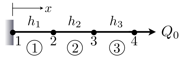
"Until now, specific applications have not been considered. Thus, the finite element equations developed are valid for any problem modeled by the governing differential equation. The only difference between different application problems is in the specification of the problem data and the boundary conditions. We next consider a four node/three element domain, as shown\n",
"\n",
"
\n",
"\n",
"The derivation of the finite element equations, i.e., the set of algebraic equations which relate the value of the primary variable to the secondary variables at the nodes, will be done using the following steps:\n",
"\n",
"**a)** Construct the weak form of the governing differential equation\n",
"\n",
"**b)** Assume the form of the approximate solution over a typical element \n",
"\n",
"**c)** Derive the FE equations by substituting the assumed form of the solution into the weak form of the governing DE \n",
"\n",
"### a) Construct the weak form of the governing differential equation\n",
"\n",
"The governing differential equation and associated boundary conditions is called the ''strong form'' of the governing equations. The ''weak'' form of the governing differential equation lends itself more easily to the finite element method. The motivation for doing this will be discussed after deriving the weak form.\n",
"\n",
"Recall the strong form of the governing differential equation:\n",
"\n",
"$$ \\frac{d}{dx}\\left( a\\frac{du}{dx}\\right) -cu+ q = 0 $$\n",
"\n",
"The weak form is derived following the three step process in [Lesson 7](Lesson7_TheWeakForm.ipynb). Namely, we first multiply the differential equation by a weight function and integrate over the problem domain\n",
"\n",
"$$ \n",
"\\int_{0}^{L}\\left( \\frac{d}{dx}\\left( a\\frac{du}{dx}\\right) -cu+ q \\right) w(x) dx=0 \n",
"$$\n",
"\n",
"Since $w(x)$ is a function of only $x$ we will write it simply as $w$. Recall that we can write this integral as\n",
"\n",
"$$\n",
" \\int_{0}^{L}\\left( \\frac{d}{dx}\\left( a\\frac{du}{dx}\\right) -cu+ q \\right) w dx= \\sum_e\\int_{\\Omega_e}\\left( \\frac{d}{dx}\\left( a\\frac{du}{dx}\\right) -cu+ q \\right) w dx=0\n",
"$$\n",
"\n",
"where $\\Omega_e=[x_1^{(e)}, x_2^{(e)}]$ is an individual element domain. Concentrating only on the $e^{\\text{th}}$ element, we have\n",
"\n",
"$$\n",
" \\int_{x_1^{(e)}}^{x_2^{(e)}} \\left( \\frac{d}{dx}\\left( a\\frac{du}{dx}\\right) w -cwu+ qw \\right)dx=0\n",
"$$\n",
"\n",
"Integrating the above expression by parts to transfer a derivative from $u$ to $w$, gives\n",
"\n",
"$$\n",
" = \\int_{x_1^{(e)}}^{x_2^{(e)}} \\frac{d}{dx}\\left( aw\\frac{du}{dx}\\right)dx - \\int_{x_1^{(e)}}^{x_2^{(e)}} a\\frac{du}{dx}\\frac{dw}{dx}dx + \\int_{x_1^{(e)}}^{x_2^{(e)}}\\left( qw -cwu \\right)dx =0\n",
"$$\n",
"\n",
"$$\n",
" \\left( aw\\frac{du}{dx} \\right) \\Bigg|_{x_1^{(e)}}^{x_2^{(e)}} - \\int_{x_1^{(e)}}^{x_2^{(e)}}{ a\\frac{du}{dx}\\frac{dw}{dx}dx} + \\int_{x_1^{(e)}}^{x_2^{(e)}}\\left( qw-cwu \\right) \\,\\mathrm{d}{x} =0\n",
"$$\n",
"\n",
"re-arranging\n",
"\n",
"$$\n",
" \\int_{x_1^{(e)}}^{x_2^{(e)}}\\left( a\\frac{du}{dx}\\frac{dw}{dx}+cwu-qw \\right)dx - wa\\frac{du}{dx}\\Bigg|_{x_1^{(e)}}^{x_2^{(e)}} =0 \n",
"$$\n",
"\n",
"Note that the essential and natural boundary conditions of the strong from arise naturally in the weak formulation. The classification of essential and natural boundary conditions is an important part of the variational formulation of the governing DE, thus we spend a moment going over the rules of their classification.\n",
"After trading differentiation between the weight function and the dependent variable, examine all boundary terms of the integral statement. The boundary terms will always involve both the weight function and the dependent variable. Coefficients of the weight function and its derivatives in the boundary expressions are termed the *secondary variables* and their specification on the boundary constitutes the *natural boundary conditions*. For our case, the boundary term $w(adu/dx)$ tells us that $adu/dx$ is the secondary variable and its specification on the boundary is the natural boundary condition.\n",
"The secondary variables always have physical meaning. In the case of heat transfer problems, the secondary variable represents heat, $Q$. We shall denote the secondary variable by\n",
"\n",
"\n",
"$$\n",
" Q=\\left( a \\frac{du}{dx} \\right) n_x\n",
"$$\n",
"\n",
"\n",
"where $n_x$ denotes the direction cosine, i.e., the angle between the $x$ axis and the normal to the boundary. For one dimensional problems, the normal is always along the length of the domain. Thus, $n_x=-1$ at the left end and $n_x=1$ at the right end of the domain.\n",
"The dependent variable of the problem, expressed in the same form as the weight function appearing in the boundary term, is called the *primary variable* and its specification on the boundary constitutes the *essential boundary conditions*. For the case in consideration, the weight function appears in the boundary expression as $w$. Therefore, the dependent variable $u$ is the primary variable and the essential boundary condition involves specifying $u$ at the boundary points.\n",
"\n",
"It should be noted that the number and form of the primary and secondary variables depend on the order of the differential equation. The number of primary and secondary variables is always the same and with each primary variable there is an associated secondary variable. For example - force and displacement, and heat and temperature. Only one of the pair, either the primary or the seondary variable, may be specified at a point of the boundary. Thus, a given problem can have its specified boundary conditions in one of three categories:\n",
"\n",
"\n",
"- All specified boundary conditions are essential (Dirichlet boundary conditions)\n",
"- Specified boundary conditions contain both essential and natural boundary conditions (mixed boundary conditions)\n",
"- All specified boundary conditions are natural (Von Neumann boundary conditions)\n",
"\n",
"\n",
"In general, a $2m^{\\rm th}$-order DE has $m$ primary variables and $m$ secondary variables.\n",
"In general, because $w$ is required to satisfy the boundary conditions of the problem the specification of $w$ and any of its derivatives constitute the essential boundary conditions. Likewise, the coefficients of $w$ or any of its derivatives constitute the natural boundary conditions.\n",
"If we now assume that all boundary conditions at the element level are of the natural type, we can re-write the term on the right hand side as\n",
"\n",
"\n",
"$$\n",
" aw\\frac{du}{dx}\\Bigg|_{x_1^{(e)}}^{x_2^{(e)}} = w(x_2^{(e)})Q_{{e+1}} + w(x_{e})Q_{{e}}\n",
"$$\n",
"\n",
"\n",
"and finally,\n",
"\n",
"\n",
"$$\n",
" \\int_{x_1^{(e)}}^{x_2^{(e)}} \\left( a\\frac{du}{dx}\\frac{dw}{dx}+cwu-wq\\right)dx - w(x_1^{(e)})Q_{{e}} - w(x_2^{(e)})Q_{{e+1}} =0\n",
"$$\n",
"\n",
"which is the weak form of the differential equation on element $e$. \n",
"\n",
"Recall that in the strong form the solution $u\\in C^1$ but in the weak form, because differentiation was transferred from $u$ to $w$, the continuity requirements were weakend so that now $u\\in C^0$. Weak and strong have nothing to do with the physical stature of the equation, only the continuity requirements on the solution.\n",
"\n",
"### b) Assume the form of the approximate solution over a typical element\n",
"\n",
"Note that the weak form over an element is equivalent to the differential equation and the natural boundary conditions on the element. However, the essential boundary conditions, $u(x_1^{(e)})=u_1^{(e)}$ and $u(x_2^{(e)})=u_2^{(e)}$, are not included in the weak form. Hence, as per our discussion of weighted residual methods, the approximation of $u$ must satisfy the essential boundary condtions. In other words, if $U_N^{(e)}$ is an approximation to $u$ on $\\Omega_{e}$ than it must be an interpolant between the nodes of the element, i.e., it must be equal to $u_1$ at $x_1^{(e)}$ and $u_2$ at $x_2^{(e)}$.\n",
"\n",
"We will now **assume** an approximate solution $U_N^{(e)}$ in the form of algebraic polynomials. We choose polynomials for two reasons - first, polynomials that satisfy the essential boundary conditions are easy to find over an element; second, integration of algebraic polynomials is easy. As in the weighted residual methods, the approximate solution must satisfy the following requirements:\n",
"\n",
"- The approximate solution should be continuous over the element and differentiable, as required by the weak form\n",
"- It must form a \"complete basis\" for the function space from which it is chosen\n",
"- It should be an interpolant of the primary variables at the nodes of the finite element\n",
"\n",
"The first requirement ensures a nonzero coefficient matrix and the third requirement is necessary in order to satisfy the essential boundary conditions of the element and to enforce continuity of the primary variables at points common to several elements. Let us now turn our attention to the second requirement. The second requirement is necessary to capture all possible states, i.e., constant, linear, and so on, of the actual solution. An approximation function forms a complete basis if it is capable of converging to any continuous function as terms are added. For example, the displacement function\n",
"\n",
"\n",
"$$\n",
" \\psi = c_0 + c_1 x + \\cdots + c_nx^n\n",
"$$\n",
"\n",
"\n",
"is complete because as $k\\rightarrow\\infty$ $u$ becomes a Taylor series which is capable of converging on any (well behaved) function. However, the displacement function\n",
"\n",
"\n",
"$$\n",
" \\psi = c_0 + c_4x^4 + \\cdots + c_nx^n\n",
"$$\n",
"\n",
"\n",
"is not a complete basis because it is missing the $c_1x, \\ c_2x^2,$ and $c_3x^3$ terms.\n",
"For the weak form of the governing equation, the minimum polynomial order required of the approximate solution is linear. Thus, a complete linear polynomial will have the form:\n",
"\n",
"\n",
"$$\n",
" ^{(e)}=a_1 + a_2x, \\ \\ \\ \\ a_1,a_2\\in{\\rm I\\kern-.16em R}\n",
"$$\n",
"\n",
"Note that this satisfies the first two requirements. Also note that there are two unknown coefficients $a_1,a_2$. We find the unknown coefficients by demanding that our approximate solution satisfies the third requirement:\n",
"\n",
"\n",
"$$\n",
" U_N^{(e)}(x_1^{(e)})=u_1^{(e)}, \\ \\ \\ \\ U_N^{(e)}(x_2^{(e)})=u_{2}^{(e)}\n",
"$$\n",
"\n",
"this now gives a relationship between the constants $a_1,a_2$ and the displacements $u_1^{(e)},u_{2}^{(e)}$\n",
"\n",
"\n",
"$$\n",
" U_N^{(e)}(x_1^{(e)})=u_1^{(e)}=a_1+a_2x_1^{(e)}\n",
"$$\n",
"\n",
"\n",
"\n",
"\n",
"$$\n",
" U_N^{(e)}(x_2^{(e)})=u_{2}^{(e)}=a_1+a_2x_2^{(e)}\n",
"$$\n",
"\n",
"\n",
"or, in matrix form\n",
"\n",
"\n",
"$$\n",
" \\left\\{ \\begin{array}{c} u_1^{(e)} \\\\ u_{2}^{(e)} \\end{array} \\right\\} = \\left[\\begin{array}{cc} 1 & x_1^{(e)} \\\\ 1 & x_2^{(e)} \\end{array} \\right] \\left\\{ \\begin{array}{c} a_1 \\\\ a_2 \\end{array} \\right\\}\n",
"$$\n",
"\n",
"\n",
"Solving for $a_1$ and $a_2$ gives\n",
"\n",
"\n",
"$$\n",
" a_1= \\frac{u_1^{(e)}x_2^{(e)}-u_{2}^{(e)}x_1^{(e)}}{x_2^{(e)}-x_1^{(e)}}\n",
"$$\n",
"\n",
"\n",
"\n",
"\n",
"$$\n",
" a_2=\\frac{u_{2}^{(e)}-u_1^{(e)}}{x_2^{(e)}-x_1^{(e)}}\n",
"$$\n",
"\n",
"\n",
"and\n",
"\n",
"\n",
"$$\n",
" U_N^{(e)} = \\frac{u_1^{(e)}x_2^{(e)}-u_{2}^{(e)}x_1^{(e)}}{x_2^{(e)}-x_1^{(e)}} + \\frac{u_{2}^{(e)}-u_1^{(e)}}{x_2^{(e)}-x_1^{(e)}}x\n",
"$$\n",
"\n",
"\n",
"after some re-arranging, the approximate solution can be written\n",
"\n",
"\n",
"$$\n",
" U_N^{(e)} = N_1^{(e)} u_1^{(e)} + N_{2}^{(e)} u_{2}^{(e)}\n",
"$$\n",
"\n",
"where\n",
"\n",
"\n",
"$$\n",
" N_1^{(e)}(x) = \\frac{x_2^{(e)}-x}{h_e}, \\qquad\n",
" N_{2}^{(e)}(x) = \\frac{x-x_1^{(e)}}{h_e}\n",
"$$\n",
"\n",
"and\n",
"\n",
"\n",
"$$\n",
" h_e = x_2^{(e)}-x_1^{(e)}\n",
"$$\n",
"\n",
"\n",
"is the length of the element. These equations are the general linear finite element approximation functions. Note that these equations are the Lagrange interpolation functions for the nodes of the elements.\n",
"\n",
"We further simplify the notation by noting that the element interpolation functions $N_i^{(e)}$ are expressed in terms of the *global coordinates* $x$ (i.e., the coordinate of the problem), but they are defined only on the element domain $\\Omega^{(e)}=(x_1^{(e)},x_2^{(e)})$. If we choose to express them in terms of a coordinate $\\hat{x}$ with origin fixed at node 1 of the element, the $N_i^{(e)}$ take the following forms\n",
"\n",
"$$ N_1^{(e)}(x)\\Rightarrow N_1^{(e)}(\\hat{x}) =\\frac{x_2-\\hat{x}}{h_e}=1-\\frac{\\hat{x}}{h_e} $$\n",
"$$ N_{2}^{(e)}(x)\\Rightarrow N_2^{(e)}(\\hat{x})=\\frac{\\hat{x}-x_1}{h_e}=\\frac{\\hat{x}}{h_e} $$\n",
"\n",
"We call the coordinate $\\hat{x}$ the *local* or *element coordinate*. Note that $N_1^{(e)}$ is equal to one at node one and zero at node two and $N_2^{(e)}$ is equal to zero at node one and one at node two. In other words, $N_i^{(e)}$ are interpolation functions of $u$. This property can be written as\n",
"\n",
"\n",
"\n",
"$$\n",
" N_i^{(e)}(x_j) = \\left\\{ \\begin{array}{c} 1 \\ \\ {\\rm if} \\ i=j \\\\ 0 \\ \\ {\\rm if} \\ i\\neq j \\end{array} \\right.\n",
"$$\n",
"\n",
"Using the local form of the interpolation functions, the approximate solution $U_N^{(e)}$ is written\n",
"\n",
"\n",
"$$\n",
" U_N^{(e)}=\\left[ \\begin{array}{cc}N_1^{(e)} & N_2^{(e)} \\end{array} \\right] \\left\\{ \\begin{array}{c} u_1^{(e)} \\\\[8pt] u_2^{(e)} \\end{array} \\right\\}\n",
"$$\n",
"\n",
"or, in a more compact form, we write\n",
"\n",
"\n",
"$$\n",
" U_N^{(e)}=\\sum_{j=1}^2 u_j^{(e)}N_j^{(e)}\n",
"$$\n",
"\n",
"\n",
"\n",
"## c) The Finite Element Model\n",
"\n",
"The weak form is equivalent to the governing differential equation over the element $\\Omega^{(e)}$ and also contains the natural boundary conditions. Further, the finite element approximation satisfies the essential boundary conditions of the element. Choosing a sufficient number of weight functions gives the necessary algebraic equations to determine the nodal values $u_i^{(e)}$ and $Q_i^{(e)}$ of the element $\\Omega^{(e)}$.\n",
"\n",
"Following the Galerkin method, we choose\n",
"\n",
"$$\n",
"w = \\sum_{i=1}^2w_i^{(e)}N_i^{(e)}\n",
"$$\n",
"\n",
"After substitution\n",
"\n",
"$$\n",
" \\int_{x_1^{(e)}}^{x_2^{(e)}}\\left( a\\frac{d\\left({\\sum_{i=1}^{2}w_i^{(e)}N_i^{(e)}}\\right)}{dx}\\frac{d\\left( {\\sum_{j=1}^{2}u_j^{(e)}N_j^{(e)}}\\right)}{dx}+ c\\sum_{i=1}^{2}w_i^{(e)}N_i^{(e)}\\sum_{j=1}^{2}u_j^{(e)}N_j^{(e)}- q\\sum_{i=1}^{2}w_i^{(e)}N_i^{(e)} \\right) \\,\\mathrm{d}{x}\n",
" - \\sum_{i=1}^{2}w_i^{(e)}N_i^{(e)}(x_1^{(e)})Q_1^{(e)}-\\sum_{i=1}^{2}w_i^{(e)}N_i^{(e)}(x_2^{(e)})Q_2^{(e)}=0\n",
"$$\n",
"\n",
"$$\n",
" =\\int_{x_1^{(e)}}^{x_2^{(e)}} \\left( a\\sum_{i=1}^2w_i^{(e)}\\sum_{j=1}^2u_j^{(e)}\\frac{dN_i^{(e)}}{dx}\\frac{dN_j^{(e)}}{dx}+ c\\sum_{i=1}^{2}w_i^{(e)}N_i^{(e)}\\sum_{j=1}^{2}u_j^{(e)}N_j^{(e)}- q\\sum_{i=1}^2w_i^{(e)}N_i^{(e)} \\right)\\,\\mathrm{d}{x}\n",
" - \\sum_{i=1}^{2}w_i^{(e)}\\left( N_i^{(e)}(x_1^{(e)})Q_1^{(e)} + N_i^{(e)}(x_2^{(e)})Q_2^{(e)} \\right)=0\n",
"$$\n",
"\n",
"$$\n",
" =\\sum_{i=1}^2w_i^{(e)}\\left[ \\int_{x_1^{(e)}}^{x_2^{(e)}}\\left( a\\sum_{j=1}^2u_j^{(e)}\\frac{dN_i^{(e)}}{dx}\\frac{dN_j^{(e)}}{dx}+cN_i^{(e)}\\sum_{j=1}^{2}u_j^{(e)}N_j^{(e)} - qN_i^{(e)} \\right)\\,\\mathrm{d}{x} - N_i^{(e)}(x_1^{(e)})Q_1^{(e)} -N_i^{(e)}(x_2^{(e)})Q_2^{(e)}\\right] =0\n",
"$$\n",
"\n",
"$$\n",
" =\\int_{x_1^{(e)}}^{x_2^{(e)}}\\left( a \\sum_{j=1}^2u_j^{(e)}\\frac{dN_i^{(e)}}{dx}\\frac{dN_j^{(e)}}{dx}+cN_i^{(e)}\\sum_{j=1}^{2}u_j^{(e)}N_j^{(e)} - qN_i^{(e)} \\right)\\,\\mathrm{d}{x}- N_i^{(e)}(x_1^{(e)})Q_1^{(e)} -N_i^{(e)}(x_2^{(e)})Q_2^{(e)} =0\n",
"$$\n",
"\n",
"Re-arranging\n",
"\n",
"$$\n",
" \\sum_{j=1}^2u_j^{(e)}\\int_{x_1^{(e)}}^{x_2^{(e)}}\\left( a \\frac{dN_i^{(e)}}{dx}\\frac{dN_j^{(e)}}{dx}+cN_i^{(e)}N_j^{(e)}\\right)\\,\\mathrm{d}{x} = \\int_{x_1^{(e)}}^{x_2^{(e)}} qN_i^{(e)} \\,\\mathrm{d}{x} \\ +\\ N_i^{(e)}(x_1^{(e)})Q_1^{(e)} +N_i^{(e)}(x_2^{(e)})Q_2^{(e)}\n",
"$$\n",
"\n",
"It is hard to see, but this is a set of 2 equations (1 equation for each free index $i$) for the two unknowns $u_1^{(e)}$ and $u_2^{(e)}$. Let's expand to see explicitly:\n",
"\n",
"$$\n",
" i=1\\Rightarrow \\sum_{j=1}^2u_j^{(e)}\\int_{x_1^{(e)}}^{x_2^{(e)}}\\left( a \\frac{dN_j^{(e)}}{dx}\\frac{dN_1^{(e)}}{dx}+cN_1^{(e)}N_j^{(e)}\\right)\\,\\mathrm{d}{x} = \\int_{x_1^{(e)}}^{x_2^{(e)}} qN_1^{(e)} \\,\\mathrm{d}{x} \\ +\\ N_1^{(e)}(x_1^{(e)})Q_1^{(e)} +N_1^{(e)}(x_2^{(e)})Q_2^{(e)}\n",
"$$\n",
"\n",
"$$\n",
" i=2\\Rightarrow \\sum_{j=1}^2u_j^{(e)}\\int_{x_1^{(e)}}^{x_2^{(e)}}\\left( a \\frac{dN_j^{(e)}}{dx}\\frac{dN_2^{(e)}}{dx}+cN_2^{(e)}N_j^{(e)}\\right)\\,\\mathrm{d}{x} = \\int_{x_1^{(e)}}^{x_2^{(e)}} qN_2^{(e)} \\,\\mathrm{d}{x} \\ +\\ N_2^{(e)}(x_1^{(e)})Q_1^{(e)} +N_2^{(e)}(x_2^{(e)})Q_2^{(e)}\n",
"$$\n",
"\n",
"These equations can now be written as\n",
"\n",
"$$\n",
" \\sum_{j=1}^2u_j^{(e)}\\int_{x_1^{(e)}}^{x_2^{(e)}}\\left( a \\frac{dN_j^{(e)}}{dx}\\frac{dN_1^{(e)}}{dx}+cN_1^{(e)}N_j^{(e)}\\right)\\,\\mathrm{d}{x} = \\int_{x_1^{(e)}}^{x_2^{(e)}} qN_1^{(e)} \\,\\mathrm{d}{x} \\ +\\ Q_1^{(e)}\n",
"$$\n",
"\n",
"$$\n",
" \\sum_{j=1}^2u_j^{(e)}\\int_{x_1^{(e)}}^{x_2^{(e)}}\\left( a \\frac{dN_j^{(e)}}{dx}\\frac{dN_2^{(e)}}{dx}+cN_2^{(e)}N_j^{(e)}\\right)\\,\\mathrm{d}{x} = \\int_{x_1^{(e)}}^{x_2^{(e)}} qN_2^{(e)} \\,\\mathrm{d}{x} \\ +\\ Q_2^{(e)}\n",
"$$\n",
"\n",
"\n",
"Which emits the following compact form of the finite element equations\n",
"\n",
"$$\n",
" k^{(e)}_{ij}u_j^{(e)} = f_i^{(e)} + Q_i^{(e)}\n",
"$$\n",
"\n",
"where\n",
"\n",
"$$\n",
" k^{(e)}_{ij}=\\int_{x_1^{(e)}}^{x_2^{(e)}} \\left( a\\frac{dN_i^{(e)}}{dx}\\frac{dN_j^{(e)}}{dx} + cN_i^{(e)}N_j^{(e)}\\right) \\,\\mathrm{d}{x}\n",
"$$\n",
"\n",
"and\n",
"\n",
"$$\n",
" f_i^{(e)}=\\int_{x_1^{(e)}}^{x_2^{(e)}} qN_i^{(e)} \\,\\mathrm{d}{x}\n",
"$$\n",
"\n",
"Recall that the $u_j$ are the unknown coefficients of our approximate solution. In matrix notation we write\n",
"\n",
"$$\n",
" [k^{(e)}]\\{u^{(e)}\\}=\\{f^{(e)}\\} + \\{Q^{(e)}\\}\n",
"$$\n",
"\n",
"\n",
"and in direct notation\n",
"\n",
"$$\n",
" {\\boldsymbol{k}}^{(e)}{\\boldsymbol{u}}^{(e)}={\\boldsymbol{f}}^{(e)} + {\\boldsymbol{Q}}^{(e)}\n",
"$$"
]
},
{
"cell_type": "markdown",
"metadata": {},
"source": [
"## Assemble Global Equations\n",
"\n",
"The global equations are assembled as\n",
"\n",
"\n",
"$$\n",
" \\int_{0}^{L}\\left( \\frac{d}{dx}\\left( a\\frac{du}{dx}\\right) -cu+ q \\right) w \\,\\mathrm{d}{x}= \\sum_e\\int_{\\Omega_e}\\left( \\frac{d}{dx}\\left( a\\frac{du}{dx}\\right) -cu+ q \\right) w dx=0\n",
"$$\n",
"\n",
"$$\n",
" \\sum_e k^{(e)}_{ij}u_j^{(e)} = \\sum_e \\left( f_i^{(e)} + Q_i^{(e)}\\right)\n",
"$$\n",
"\n",
"As with the direct method, the local stiffness matrices and force arrays are expanded and summed to produce the global equations:\n",
"\n",
"$$\n",
" k_{ij}=\\sum_{e=1}^{N-1}k_{ij}^{(e)}=\\left[\\begin{array}{ccccccccccc}\n",
" {k_{11}^{(1)}} & {k_{12}^{(1)}} & 0 & \\cdots &\\cdots & \\cdots& \\cdots& \\cdots & 0\\\\\n",
" {k_{21}^{(1)}} & {k_{22}^{(1)}}+{k_{11}^{(2)}}&{k_{12}^{(2)}}& 0 &\\cdots & \\cdots&\\cdots&\\cdots &0 \\\\\n",
" 0 & {k_{21}^{(2)}}&{k_{22}^{(2)}}+{k_{11}^{(3)}}&{k_{12}^{(3)}}& 0 &\\cdots&\\cdots& \\cdots&0 \\\\\n",
" 0 & \\cdots & \\ddots & \\ddots & \\ddots & 0&\\cdots&\\cdots & 0\\\\\n",
" 0 & \\cdots& \\cdots & {k_{21}^{(e-1)}}&{k_{22}^{(e-1)}}+{k_{11}^{(e)}}&{k_{12}^{(e)}}& 0 &\\cdots &0 \\\\\n",
" 0 & \\cdots& \\cdots & \\cdots & \\ddots & \\ddots&\\ddots&\\cdots&0\\\\\n",
" 0 & \\cdots&\\cdots& \\cdots & \\cdots&\\cdots &\\cdots&{k_{21}^{(N-1)}} &{k_{22}^{(N-1)}} \\\\\n",
" \\end{array} \\right]\n",
"$$\n",
"\n",
"$$\n",
" f_i=\\left\\{ \\begin{array}{c} f_1^1 \\\\ f_2^1+f_1^2 \\\\ f_2^2+f_1^{(3)} \\\\ \\vdots \\\\ f_2^{(e-1)}+f_1^{(e)} \\\\ \\vdots \\\\ f_2^{(N-1)} \\end{array} \\right\\}, \\ \\ \\ \\\n",
" Q_i=\\left\\{ \\begin{array}{c} Q_1^1 \\\\ Q_2^1+Q_1^2 \\\\ Q_2^2+Q_1^{(3)} \\\\ \\vdots \\\\ Q_2^{(e-1)}+Q_1^{(e)} \\\\ \\vdots \\\\ Q_2^{(N-1)} \\end{array} \\right\\}\n",
"$$\n",
"\n",
"then,\n",
"\n",
"$$\n",
" \\left[\\begin{array}{ccccccccccc}\n",
" {k_{11}^{(1)}} & {k_{12}^{(1)}} & 0 & \\cdots &\\cdots & \\cdots& \\cdots& \\cdots & 0\\\\\n",
" {k_{21}^{(1)}} & {k_{22}^{(1)}}+{k_{11}^{(2)}}&{k_{12}^{(2)}}& 0 &\\cdots & \\cdots&\\cdots&\\cdots &0 \\\\\n",
" 0 & {k_{21}^{(2)}}&{k_{22}^{(2)}}+{k_{11}^{(3)}}&{k_{12}^{(3)}}& 0 &\\cdots&\\cdots& \\cdots&0 \\\\\n",
" 0 & \\cdots & \\ddots & \\ddots & \\ddots & 0&\\cdots&\\cdots & 0\\\\\n",
" 0 & \\cdots& \\cdots & {k_{21}^{(e-1)}}&{k_{22}^{(e-1)}}+{k_{11}^{(e)}}&{k_{12}^{(e)}}& 0 &\\cdots &0 \\\\\n",
" 0 & \\cdots& \\cdots & \\cdots & \\ddots & \\ddots&\\ddots&\\cdots&0\\\\\n",
" 0 & \\cdots&\\cdots& \\cdots & \\cdots&\\cdots &\\cdots&{k_{21}^{(N-1)}} &{k_{22}^{(N-1)}} \\\\\n",
" \\end{array} \\right] \\left\\{ \\begin{array}{c} u_1 \\\\ u_2 \\\\ u_3 \\\\ \\vdots \\\\ u_{e} \\\\ \\vdots \\\\ u_{N} \\end{array} \\right\\}\n",
"$$\n",
"$$\n",
" =\n",
" \\left\\{ \\begin{array}{c} f_1^{(1)} \\\\ f_2^{(1)}+f_1^{(2)} \\\\ f_2^{(2)}+f_1^{(3)} \\\\ \\vdots \\\\ f_2^{(e-1)}+f_1^{(e)} \\\\ \\vdots \\\\ f_2^{(N-1)} \\end{array} \\right\\} +\n",
" \\left\\{ \\begin{array}{c} Q_1^{(1)} \\\\ Q_2^{(1)}+Q_1^{(2)} \\\\ Q_2^{(2)}+Q_1^{(3)} \\\\ \\vdots \\\\ Q_2^{(e-1)}+Q_1^{(e)} \\\\ \\vdots \\\\ Q_2^{(N-1)} \\end{array} \\right\\}\n",
"$$\n",
"\n",
"Note that in the derivation of the global equations it was assumed that the nodes were connected in series numbered in sequentially. As was seen with the direct stiffness method, it is possible to have elements connected in parallel and for the nodes to be numbered randomly. In that case, the ideas in the above expression hold, but the order of the coefficients in the different matrices will be changed accordingly."
]
},
{
"cell_type": "markdown",
"metadata": {},
"source": [
"## Element Connectivity\n",
"\n",
"When deriving the element equation for our governing equation, the $e^{\\rm th}$ element of the finite element mesh was isolated. To solve the global system, the element is put back into its original position and following two conditions (assuming that the nodes and elements are numbered in sequence) are enforced:\n",
"\n",
"- Continuity of primary variables at connecting nodes:\n",
" $$\n",
" {u_n^{(e)}=u_1^{(e+1)}}\n",
" $$\n",
" i.e., the last nodal value of the element $\\Omega^{(e)}$ is the same as the first nodal value of the adjacent element $\\Omega^{(e+1)}$.\n",
"\n",
"- Balance of secondary variables at connecting nodes:\n",
" $$\n",
" Q_n^{(e)}+Q_1^{(e+1)}=\\left\\{\\begin{array}{cl} 0 & {\\rm if \\ no \\ external \\ point \\ source \\ is \\ applied}\\\\ Q_0 & {\\rm if \\ an \\ external \\ point \\ source \\ of \\ magnitude } \\\\ & Q_0 {\\rm \\ is \\ applied}\\end{array} \\right.\n",
" $$\n",
"\n",
"The first condition merely states that the value of the primary variable is continuous over the problem domain and is enforced as\n",
"\n",
"$$\n",
" u_n^{(e)}=u_1^{(e+1)}=u_N\n",
"$$\n",
"\n",
"where $N$ is the global node number for the connecting node and is given by $N=(n-1)e+1$. For example, for a mesh of three linear ($n=2$) finite elements\n",
"\n",
"$$\n",
" \\begin{array}{c}\n",
" u_1^{(1)}=u_1 \\\\\n",
" u_2^{(1)}+u_1^{(2)}=u_2 \\\\\n",
" u_2^{(2)}+u_1^{(3)}=u_3 \\\\\n",
" u_2^{(3)}=u_4\n",
" \\end{array}\n",
"$$\n",
"\n",
"The second condition says that the value of the derivative of the primary variable is continuous at the point common to to elements $\\Omega^{(e)}$ and $\\Omega^{(e+1)}$ (when no change in $du/dx$ is imposed externally):\n",
"\n",
"$$\n",
" \\left( \\frac{du}{dx}\\right)^{(e)}=\\left( \\frac{du}{dx}\\right)^{(e+1)}\n",
"$$\n",
"$$\n",
" \\left( \\frac{du}{dx}\\right)^{(e)}+\\left( -\\frac{du}{dx}\\right)^{(e+1)}=0\n",
"$$\n",
"$$\n",
" \\Rightarrow Q_2^{(e)}+Q_1^{(e+1)}=0\n",
"$$"
]
},
{
"cell_type": "markdown",
"metadata": {},
"source": [
"# Examples [](#top)"
]
},
{
"cell_type": "markdown",
"metadata": {},
"source": [
"## Example: Linear Element Stiffness \n",
"\n",
"The stiffness matrix for the linear element can be determined in the local coordinates\n",
"\n",
"$$\n",
" k^{(e)}_{ij}=\\int_{0}^{h_e} \\left( a_1\\frac{dN_i^{(e)}}{d\\hat x}\\frac{dN_j^{(e)}}{d\\hat x} + c_1N_i^{(e)}N_j^{(e)}\\right) d\\hat x\n",
"$$\n",
"\n",
"It may not be obvious that $dx$ can be replaced with $d\\hat{x}$. Note that $\\hat{x}=x-x_1^{(e)}$, then $d\\hat{x}=dx$. Similar arguments can show that $dN_i^{(e)}/dx=dN_i^{(e)}/d\\hat{x}$. \n",
"\n",
"The coefficients of the stiffness are then found as\n",
"\n",
"$$\n",
" k^{(e)}_{11}=\\int_0^{h_e} a_1\\left(-\\frac{1}{h_e}\\right)\\left(-\\frac{1}{h_e}\\right) +c_1\\left( 1-\\frac{\\hat x}{h_e}\\right)\\left( 1-\\frac{\\hat x}{h_e}\\right) d\\hat{x} = \\frac{a_1}{h_e}+\\frac{1}{3}c_1h_e\n",
"$$\n",
"\n",
"$$\n",
" k^{(e)}_{12}=\\int_0^{h_e} a_1\\left(-\\frac{1}{h_e}\\right)\\left(\\frac{1}{h_e}\\right) +c_1\\left( 1-\\frac{\\hat x}{h_e}\\right)\\left(\\frac{\\hat x}{h_e}\\right) d\\hat{x} = \\frac{a_1}{h_e}+\\frac{1}{6}c_1h_e\n",
"$$\n",
"\n",
"$$\n",
" k^{(e)}_{21}=k^{(e)}_{12}\n",
"$$\n",
"\n",
"$$\n",
" k^{(e)}_{22}=\\int_0^{h_e} a_1\\left(\\frac{1}{h_e}\\right)\\left(\\frac{1}{h_e}\\right) +c_1\\left( \\frac{\\hat x}{h_e}\\right)\\left( \\frac{\\hat x}{h_e}\\right) d\\hat{x} = \\frac{a_1}{h_e}+\\frac{1}{3}c_1h_e\n",
"$$\n",
"\n",
"Similarly, if $q$ is constant over the element\n",
"\n",
"$$\n",
" f_1^{(e)} = \\int_0^{h_e}q_1\\left( 1-\\frac{\\hat{x}}{h_e} \\right) d\\hat{x}=\\frac{1}{2} q_1h_e\n",
"$$\n",
"\n",
"$$\n",
" f_2^{(e)} = \\int_0^{h_e}q_1\\frac{\\hat{x}}{h_e} d\\hat{x}=\\frac{1}{2} q_1h_e\n",
"$$\n",
"\n",
"Thus, for a constant $q_1$, the total source $q_1h_e$ is equally distributed to the two nodes. The coefficient matrix and column vector are then\n",
"\n",
"$$\n",
" {\\boldsymbol{k}}^{(e)}=\\frac{a_1}{h_e}\\left[\\begin{array}{cc} 1 & -1 \\\\ -1 & 1 \\end{array} \\right] +\\frac{c_1h_e}{6}\\left[\\begin{array}{cc} 2 & 1 \\\\ 1 & 2 \\end{array} \\right]\n",
"$$\n",
"\n",
"$$\n",
" {\\boldsymbol{f}}^{(e)}= \\frac{q_1h_e}{2}\\left\\{\\begin{array}{c} 1 \\\\ 1 \\end{array} \\right\\}\n",
"$$\n",
"\n",
"The form of ${\\boldsymbol{Q}}^{(e)}$ will be investigated when the boundary conditions are considered."
]
},
{
"cell_type": "markdown",
"metadata": {},
"source": [
"## Example: Imposition of Boundary Conditions\n",
"\n",
"Until now, specific applications have not been considered. Thus, the finite element equations developed are valid for any problem modeled by the governing differential equation. The only difference between different application problems is in the specification of the problem data and the boundary conditions. We next consider a four node/three element domain, as shown\n",
"\n",
" \n",
"\n",
"The problem data are as follows: $c=q=u_1=0$. Imposing the boundary conditions on the assembled global equations we obtain\n",
"\n",
"$$ \\begin{bmatrix} \n",
"k_{11}^{(1)} & k_{12}^{(1)} & 0 & 0 \\\\ \n",
"k_{21}^{(1)} & k_{22}^{(1)} + k_{11}^{(2)} & k_{12}^{(2)} & 0 \\\\ \n",
"0 & k_{21}^{(2)} & k_{22}^{(2)}+k_{11}^{(3)} & k_{12}^{(3)} \\\\ \n",
"0 & 0 & k_{21}^{(3)} & k_{22}^{(3)} \\end{bmatrix} \n",
"\\begin{Bmatrix} 0 \\\\ u_2 \\\\ u_3 \\\\ u_4 \\end{Bmatrix} = \n",
"\\begin{Bmatrix} Q_1^{(1)} \\\\ 0 \\\\ 0 \\\\ Q_0 \\end{Bmatrix}\n",
"$$\n",
"\n",
"which contains four equations for the four unknowns $u_2, u_3, u_4 $ and $Q_1^1$."
]
},
{
"cell_type": "markdown",
"metadata": {},
"source": [
"## Example 3: Postprocessing of Solution\n",
"\n",
" The solution of the finite element equations gives the nodal values of the primary unknown (i.e., displacement, velocity, or temperature). Postprocessing of the results includes one or more of the following:\n",
"\n",
"- Computation of any secondary variables (i.e., the gradient of the solution). \n",
"- Interpretation of the results. \n",
"- Tabular and/or graphical presentation of results.\n",
"\n",
" To determine the solution of $u$ as a continuous function of position $x$, we return to the approximation for $u$\n",
" \n",
"\n",
"$$ U_N^{(e)}=\\sum_{i=1}^2 u_j^{(e)}N_j^{(e)} $$\n",
"\n",
"\n",
"over each element:\n",
"\n",
"\n",
"$$\n",
" u(x) \\approx \\left\\{ \\begin{array}{c} {\\sum_{j=1}^2 u_j^{(1)}N_j^{(1)}} \\\\ ={\\sum_{j=1}^2 u_j^{(2)}N_j^{(2)}} \\\\ \\vdots \\\\ {\\sum_{i=1}^2 u_j^{(N)}N_j^{(N)}} \\end{array} \\right.\n",
"$$\n",
"\n",
"where $N$ is the number of elements in the mesh. Depending on the value of $x$, the corresponding element equation is used. The derivative of the solution is obtained by differentiation.\n",
"\n",
"\n",
"$$\n",
" \\frac{du}{dx} \\approx \\left\\{ \\begin{array}{c} {\\sum_{j=1}^2 u_j^{(1)}\\frac{dN_j^{(1)}}{dx}} \\\\ {\\sum_{j=1}^{(2)} u_j^2\\frac{dN_j^{(2)}}{dx}} \\\\ \\vdots \\\\ {\\sum_{j=1}^2 u_j^{(N)}\\frac{dN_j^{(N)}}{dx}} \\end{array} \\right.\n",
"$$\n",
"\n",
"Note that the derivative $dU_N^{(e)}/dx$ of the linear finite element solution $U_N^{(e)}$ is constant within each element and it is discontinuous at the nodes because the continuity of the derivative of the finite element solution at the connecting nodes is not imposed:\n",
"\n",
"\n",
"$$\n",
" \\frac{dU_N^{(e)}}{dx}\\neq\\frac{dU_N^{(e+1)}}{dx}\n",
"$$\n",
"\n",
"\n",
"The derivative calculated from different elements meeting at a node is always discontinuous in all $C^0$ approximations, unless the approximate solution coincides with the actual solution.\n",
"FYI, the secondary variables $Q_i^{(e)}$ can be computed in two different ways. We can determine them directly from the assembled global equations, as we have been doing. We will denote the $Q_i^{(e)}$ found in this way as $(Q_i^{(e)})_{\\rm equil}$, since the assembled equations often represent the equilibrium relations of the system. The $Q_i^{(e)}$ can also be computed\n",
"\n",
"\n",
"$$\n",
" -Q_1^{(e)}=\\left( a\\frac{du}{dx}\\right)\\Bigg|_{x=x_1^{(e)}}, \\ \\ \\ \\ Q_2^{(e)}=\\left( a\\frac{du}{dx}\\right)\\Bigg|_{x=x_2^{(e)}}\n",
"$$\n",
"\n",
"\n",
"by replacing $u$ with $U_N$. We will denote the $Q_i^{(e)}$ found in this way as $(Q_i^{(e)})_{\\rm def}$. Since $(Q_i^{(e)})_{\\rm def}$ are calculated using the approximate $U_N$, they are not as accurate as $(Q_i^{(e)})_{\\rm equil}$. However, in finite element computer codes, $(Q_i^{(e)})_{\\rm def}$ are calculated instead of $(Q_i^{(e)})_{\\rm equil}$, for computational ease. However, in this class we will stick mainly with finding $(Q_i^{(e)})_{\\rm equil}$.\n"
]
},
{
"cell_type": "markdown",
"metadata": {},
"source": [
"# Closing Remarks\n",
"\n",
"**Remark 1.** We used the Galerkin method to derive the finite element equations, but other methods such as the Raleigh-Ritz method or least squares could have been used.\n",
"\n",
"**Remark 2.** The steps we followed today are common for any problem in the table of applications. The derivation of the interpolation functions depended only on the element geometry and on the number and position of nodes in the element.\n",
"\n",
"**Remark 3.** For more complicated elements, numerical integration will be necessary to evaluate the element matrices. We will cover this later in the semester.\n",
"\n",
"**Remark 4.** Point sources at the nodes are included in the finite element model via the balance of sources at the nodes. Thus, when constructing a finite element mesh, one should be sure to include a node at the location of a point source. There are ways to deal with point sources applied between nodes, but we won't cover them until later this semester.\n",
"\n",
"**Remark 5.** There are three types of errors associated with the finite element method:\n",
"\n",
"- Domain approximation error - error due to approximation of domain\n",
"- Computational errors - errors due to finite arithmetic\n",
"- Approximation errors - error due to approximation of continuous solution with piecewise solution\n",
"\n",
"**Remark 6.** Since $k_{ij}^{(e)}$ is symmetric, one need only compute the diagonal and the upper or lower diagonal terms. Because of the symmetry of the element matrices, the global matrix is also symmetric and one need only store the upper triangle, including the diagonal, in a finite element program. This can save a lot of memory for large systems. Also, since the global matrix $K_{IJ}=0$ if global nodes $I$ and $J$ do not belong to the same element, the global coefficient matrix is banded.\n"
]
}
],
"metadata": {
"kernelspec": {
"display_name": "Python 2",
"language": "python",
"name": "python2"
},
"language_info": {
"codemirror_mode": {
"name": "ipython",
"version": 2
},
"file_extension": ".py",
"mimetype": "text/x-python",
"name": "python",
"nbconvert_exporter": "python",
"pygments_lexer": "ipython2",
"version": "2.7.9"
}
},
"nbformat": 4,
"nbformat_minor": 0
}
\n",
"\n",
"The problem data are as follows: $c=q=u_1=0$. Imposing the boundary conditions on the assembled global equations we obtain\n",
"\n",
"$$ \\begin{bmatrix} \n",
"k_{11}^{(1)} & k_{12}^{(1)} & 0 & 0 \\\\ \n",
"k_{21}^{(1)} & k_{22}^{(1)} + k_{11}^{(2)} & k_{12}^{(2)} & 0 \\\\ \n",
"0 & k_{21}^{(2)} & k_{22}^{(2)}+k_{11}^{(3)} & k_{12}^{(3)} \\\\ \n",
"0 & 0 & k_{21}^{(3)} & k_{22}^{(3)} \\end{bmatrix} \n",
"\\begin{Bmatrix} 0 \\\\ u_2 \\\\ u_3 \\\\ u_4 \\end{Bmatrix} = \n",
"\\begin{Bmatrix} Q_1^{(1)} \\\\ 0 \\\\ 0 \\\\ Q_0 \\end{Bmatrix}\n",
"$$\n",
"\n",
"which contains four equations for the four unknowns $u_2, u_3, u_4 $ and $Q_1^1$."
]
},
{
"cell_type": "markdown",
"metadata": {},
"source": [
"## Example 3: Postprocessing of Solution\n",
"\n",
" The solution of the finite element equations gives the nodal values of the primary unknown (i.e., displacement, velocity, or temperature). Postprocessing of the results includes one or more of the following:\n",
"\n",
"- Computation of any secondary variables (i.e., the gradient of the solution). \n",
"- Interpretation of the results. \n",
"- Tabular and/or graphical presentation of results.\n",
"\n",
" To determine the solution of $u$ as a continuous function of position $x$, we return to the approximation for $u$\n",
" \n",
"\n",
"$$ U_N^{(e)}=\\sum_{i=1}^2 u_j^{(e)}N_j^{(e)} $$\n",
"\n",
"\n",
"over each element:\n",
"\n",
"\n",
"$$\n",
" u(x) \\approx \\left\\{ \\begin{array}{c} {\\sum_{j=1}^2 u_j^{(1)}N_j^{(1)}} \\\\ ={\\sum_{j=1}^2 u_j^{(2)}N_j^{(2)}} \\\\ \\vdots \\\\ {\\sum_{i=1}^2 u_j^{(N)}N_j^{(N)}} \\end{array} \\right.\n",
"$$\n",
"\n",
"where $N$ is the number of elements in the mesh. Depending on the value of $x$, the corresponding element equation is used. The derivative of the solution is obtained by differentiation.\n",
"\n",
"\n",
"$$\n",
" \\frac{du}{dx} \\approx \\left\\{ \\begin{array}{c} {\\sum_{j=1}^2 u_j^{(1)}\\frac{dN_j^{(1)}}{dx}} \\\\ {\\sum_{j=1}^{(2)} u_j^2\\frac{dN_j^{(2)}}{dx}} \\\\ \\vdots \\\\ {\\sum_{j=1}^2 u_j^{(N)}\\frac{dN_j^{(N)}}{dx}} \\end{array} \\right.\n",
"$$\n",
"\n",
"Note that the derivative $dU_N^{(e)}/dx$ of the linear finite element solution $U_N^{(e)}$ is constant within each element and it is discontinuous at the nodes because the continuity of the derivative of the finite element solution at the connecting nodes is not imposed:\n",
"\n",
"\n",
"$$\n",
" \\frac{dU_N^{(e)}}{dx}\\neq\\frac{dU_N^{(e+1)}}{dx}\n",
"$$\n",
"\n",
"\n",
"The derivative calculated from different elements meeting at a node is always discontinuous in all $C^0$ approximations, unless the approximate solution coincides with the actual solution.\n",
"FYI, the secondary variables $Q_i^{(e)}$ can be computed in two different ways. We can determine them directly from the assembled global equations, as we have been doing. We will denote the $Q_i^{(e)}$ found in this way as $(Q_i^{(e)})_{\\rm equil}$, since the assembled equations often represent the equilibrium relations of the system. The $Q_i^{(e)}$ can also be computed\n",
"\n",
"\n",
"$$\n",
" -Q_1^{(e)}=\\left( a\\frac{du}{dx}\\right)\\Bigg|_{x=x_1^{(e)}}, \\ \\ \\ \\ Q_2^{(e)}=\\left( a\\frac{du}{dx}\\right)\\Bigg|_{x=x_2^{(e)}}\n",
"$$\n",
"\n",
"\n",
"by replacing $u$ with $U_N$. We will denote the $Q_i^{(e)}$ found in this way as $(Q_i^{(e)})_{\\rm def}$. Since $(Q_i^{(e)})_{\\rm def}$ are calculated using the approximate $U_N$, they are not as accurate as $(Q_i^{(e)})_{\\rm equil}$. However, in finite element computer codes, $(Q_i^{(e)})_{\\rm def}$ are calculated instead of $(Q_i^{(e)})_{\\rm equil}$, for computational ease. However, in this class we will stick mainly with finding $(Q_i^{(e)})_{\\rm equil}$.\n"
]
},
{
"cell_type": "markdown",
"metadata": {},
"source": [
"# Closing Remarks\n",
"\n",
"**Remark 1.** We used the Galerkin method to derive the finite element equations, but other methods such as the Raleigh-Ritz method or least squares could have been used.\n",
"\n",
"**Remark 2.** The steps we followed today are common for any problem in the table of applications. The derivation of the interpolation functions depended only on the element geometry and on the number and position of nodes in the element.\n",
"\n",
"**Remark 3.** For more complicated elements, numerical integration will be necessary to evaluate the element matrices. We will cover this later in the semester.\n",
"\n",
"**Remark 4.** Point sources at the nodes are included in the finite element model via the balance of sources at the nodes. Thus, when constructing a finite element mesh, one should be sure to include a node at the location of a point source. There are ways to deal with point sources applied between nodes, but we won't cover them until later this semester.\n",
"\n",
"**Remark 5.** There are three types of errors associated with the finite element method:\n",
"\n",
"- Domain approximation error - error due to approximation of domain\n",
"- Computational errors - errors due to finite arithmetic\n",
"- Approximation errors - error due to approximation of continuous solution with piecewise solution\n",
"\n",
"**Remark 6.** Since $k_{ij}^{(e)}$ is symmetric, one need only compute the diagonal and the upper or lower diagonal terms. Because of the symmetry of the element matrices, the global matrix is also symmetric and one need only store the upper triangle, including the diagonal, in a finite element program. This can save a lot of memory for large systems. Also, since the global matrix $K_{IJ}=0$ if global nodes $I$ and $J$ do not belong to the same element, the global coefficient matrix is banded.\n"
]
}
],
"metadata": {
"kernelspec": {
"display_name": "Python 2",
"language": "python",
"name": "python2"
},
"language_info": {
"codemirror_mode": {
"name": "ipython",
"version": 2
},
"file_extension": ".py",
"mimetype": "text/x-python",
"name": "python",
"nbconvert_exporter": "python",
"pygments_lexer": "ipython2",
"version": "2.7.9"
}
},
"nbformat": 4,
"nbformat_minor": 0
}