{
"cells": [
{
"cell_type": "code",
"execution_count": 1,
"metadata": {
"collapsed": false
},
"outputs": [
{
"data": {
"text/html": [
"\n"
],
"text/plain": [
""
]
},
"execution_count": 1,
"metadata": {},
"output_type": "execute_result"
}
],
"source": [
"import theme\n",
"theme.load_style()"
]
},
{
"cell_type": "markdown",
"metadata": {},
"source": [
"# Lesson 9: Examples of One Dimensional Second Order Boundary Value Problems\n",
"\n",
" \n",
"\n",
"This lecture by Tim Fuller is licensed under the\n",
"Creative Commons Attribution 4.0 International License. All code examples are also licensed under the [MIT license](http://opensource.org/licenses/MIT)."
]
},
{
"cell_type": "markdown",
"metadata": {},
"source": [
"# Topics\n",
"- [Introduction](#intro)\n",
"- [Review](#review)\n",
"- [Heat Transfer](#heat)\n",
" - [Key Equations](#key-heat-eqns)\n",
" - [Example: Temperature Distribution in a Wall](#ex-1)\n",
"- [Fluid Mechanics](#fluid)\n",
" - [Key Equations](#bg)\n",
" - [Example: Flow Between Two Parallel Plates](#fluid-ex)\n",
"- [Solid Mechanics](#solid)\n",
" - [Key Equations](#deriv)\n",
" - [Example: Compression of Tapered Column](#solid-ex)\n",
"- [Example: Point Loads Between Nodes](#ex-ptloads)\n",
"- [Example: Axisymmetry](#axisymm)"
]
},
{
"cell_type": "markdown",
"metadata": {},
"source": [
"# Introduction[
\n",
"\n",
"This lecture by Tim Fuller is licensed under the\n",
"Creative Commons Attribution 4.0 International License. All code examples are also licensed under the [MIT license](http://opensource.org/licenses/MIT)."
]
},
{
"cell_type": "markdown",
"metadata": {},
"source": [
"# Topics\n",
"- [Introduction](#intro)\n",
"- [Review](#review)\n",
"- [Heat Transfer](#heat)\n",
" - [Key Equations](#key-heat-eqns)\n",
" - [Example: Temperature Distribution in a Wall](#ex-1)\n",
"- [Fluid Mechanics](#fluid)\n",
" - [Key Equations](#bg)\n",
" - [Example: Flow Between Two Parallel Plates](#fluid-ex)\n",
"- [Solid Mechanics](#solid)\n",
" - [Key Equations](#deriv)\n",
" - [Example: Compression of Tapered Column](#solid-ex)\n",
"- [Example: Point Loads Between Nodes](#ex-ptloads)\n",
"- [Example: Axisymmetry](#axisymm)"
]
},
{
"cell_type": "markdown",
"metadata": {},
"source": [
"# Introduction[ ](#top)\n",
"\n",
"In [Lesson 8](Lesson8_DerivationOf1DEquations.ipynb), the finite element equations for second order boundary value problems were derived. In this lesson, specific applications from heat transfer, fluid mechanics, and solid mechanics will be examined."
]
},
{
"cell_type": "markdown",
"metadata": {},
"source": [
"# Review[](#top)\n",
"\n",
"The key finite element equations are\n",
"\n",
"## Strong Form\n",
"\n",
"$$\n",
" \\frac{d}{dx}\\left( a(x) \\frac{du(x)}{dx} \\right) - c(x)u(x) + q(x) = 0 \n",
" \\quad \\text{for } x\\in(0,L)\n",
"$$\n",
"\n",
"$$\n",
" u(0)=u_0, \\ \\ \\left( a(x)\\frac{du(x)}{dx} \\right)\\Bigg|_{x=L}=Q_0\n",
"$$\n",
"\n",
"## Weak Form\n",
"\n",
"$$\n",
" \\int_{x_1}^{x_2} \\left( a\\frac{du}{dx}\\frac{dw}{dx}+cwu-wq\\right) \\,\\mathrm{d}{x} - w(x_1)Q_1 - w(x_2)Q_{2} =0\n",
"$$\n",
"\n",
"## Representative Applications\n",
"\n",
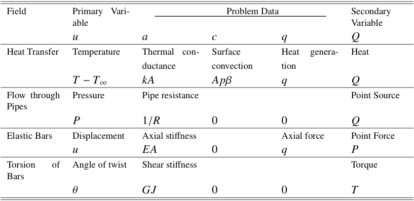
"
](#top)\n",
"\n",
"In [Lesson 8](Lesson8_DerivationOf1DEquations.ipynb), the finite element equations for second order boundary value problems were derived. In this lesson, specific applications from heat transfer, fluid mechanics, and solid mechanics will be examined."
]
},
{
"cell_type": "markdown",
"metadata": {},
"source": [
"# Review[](#top)\n",
"\n",
"The key finite element equations are\n",
"\n",
"## Strong Form\n",
"\n",
"$$\n",
" \\frac{d}{dx}\\left( a(x) \\frac{du(x)}{dx} \\right) - c(x)u(x) + q(x) = 0 \n",
" \\quad \\text{for } x\\in(0,L)\n",
"$$\n",
"\n",
"$$\n",
" u(0)=u_0, \\ \\ \\left( a(x)\\frac{du(x)}{dx} \\right)\\Bigg|_{x=L}=Q_0\n",
"$$\n",
"\n",
"## Weak Form\n",
"\n",
"$$\n",
" \\int_{x_1}^{x_2} \\left( a\\frac{du}{dx}\\frac{dw}{dx}+cwu-wq\\right) \\,\\mathrm{d}{x} - w(x_1)Q_1 - w(x_2)Q_{2} =0\n",
"$$\n",
"\n",
"## Representative Applications\n",
"\n",
" \n",
"\n",
"## Shape Functions\n",
"\n",
"Element shape functions expressed in local coordinates:\n",
"\n",
"$$N_1^{(e)}(\\hat{x}) = 1-\\frac{\\hat{x}}{h^{(e)}}$$\n",
"$$N_2^{(e)}(\\hat{x}) = \\frac{\\hat{x}}{h^{(e)}}$$\n",
"\n",
"## Stiffness Matrix\n",
"\n",
"Stiffness matrix for a single element:\n",
"\n",
"\n",
"$$\n",
" k^{(e)}_{ij}=\\int_{x_1^{(e)}}^{x_2^{(e+1)}} \\left( a^{(e)}\\frac{dN_i^{(e)}}{dx}\\frac{dN_j{(e)}}{dx} + cN_i^{(e)}N_j^{(e)}\\right) \\,\\mathrm{d}{x}\n",
"$$\n",
"\n",
"## Force Array\n",
"\n",
"Force array for a single element:\n",
"\n",
"\n",
"$$\n",
" f_i^{(e)}=\\int_{x_{1}^{(e)}}^{x_{2}^{(e)}} qN_i^{(e)} \\,\\mathrm{d}{x}\n",
"$$\n",
"\n",
"\n",
"## Finite Element Equations\n",
"\n",
"\n",
"$$\n",
" k{(e)}_{ij}u_j{(e)} = f_i^{(e)} + Q_i^{(e)}\n",
"$$\n",
"\n",
"## Assembly of Element Equations\n",
"\n",
"$$\n",
" K_{ij}=\\sum_{e=1}^{N-1}k^{(e)}_{ij}\n",
"$$\n",
"\n",
"\n",
"$$\n",
" f_j=\\sum_{e=1}^{N-1}f_i^{(e)}\n",
"$$\n",
"\n",
"\n",
"where $N$ is the number of nodes. Balance of secondary variables at connecting nodes:\n",
"\n",
"\n",
"$$\n",
" Q_2^{(e)}+Q_1^{(e+1)} = \n",
" \\begin{cases} 0 & \\text{if no external point source is applied}\\\\\n",
" Q_0 & \\text{if an external point source of magnitude } \\\\ & Q_0 \\text{ is applied}\n",
" \\end{cases}\n",
"$$"
]
},
{
"cell_type": "markdown",
"metadata": {},
"source": [
"# Heat Transfer[](#top)\n",
"\n",
"## Key Equations from Heat Transfer\n",
"\n",
"Fourier's law of conduction:\n",
"\n",
"$$\n",
" q_x=-\\kappa A \\frac{\\partial T}{{\\partial x}}\n",
"$$\n",
"\n",
"Newton's law of cooling:\n",
"\n",
"$$\n",
" q_x=\\beta A(T_s-T_{\\infty})\n",
"$$\n",
"\n",
"Change in internal energy per unit volume\n",
"\n",
"$$\n",
" \\Delta E=\\rho c_v \\frac{\\partial T}{\\partial t}\n",
"$$\n",
"\n",
"where $A$ is the element cross section, $T$ is the temperature, $\\kappa$ is the thermal conductivity, $h$ is the convection heat transfer coefficient, $\\rho$ is the density, and $c_v$ is the specific heat.\n",
"\n",
"### Derivation of Heat Equation\n",
"\n",
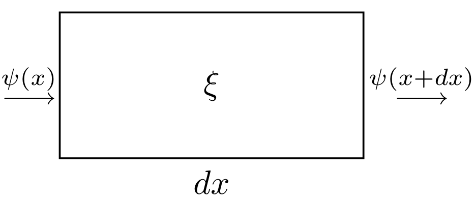
"Consider the single heat transfer element with energy entering at $x$, leaving at $x+dx$, energy transfer $\\psi$, and heat generation $\\xi$\n",
"\n",
"
\n",
"\n",
"## Shape Functions\n",
"\n",
"Element shape functions expressed in local coordinates:\n",
"\n",
"$$N_1^{(e)}(\\hat{x}) = 1-\\frac{\\hat{x}}{h^{(e)}}$$\n",
"$$N_2^{(e)}(\\hat{x}) = \\frac{\\hat{x}}{h^{(e)}}$$\n",
"\n",
"## Stiffness Matrix\n",
"\n",
"Stiffness matrix for a single element:\n",
"\n",
"\n",
"$$\n",
" k^{(e)}_{ij}=\\int_{x_1^{(e)}}^{x_2^{(e+1)}} \\left( a^{(e)}\\frac{dN_i^{(e)}}{dx}\\frac{dN_j{(e)}}{dx} + cN_i^{(e)}N_j^{(e)}\\right) \\,\\mathrm{d}{x}\n",
"$$\n",
"\n",
"## Force Array\n",
"\n",
"Force array for a single element:\n",
"\n",
"\n",
"$$\n",
" f_i^{(e)}=\\int_{x_{1}^{(e)}}^{x_{2}^{(e)}} qN_i^{(e)} \\,\\mathrm{d}{x}\n",
"$$\n",
"\n",
"\n",
"## Finite Element Equations\n",
"\n",
"\n",
"$$\n",
" k{(e)}_{ij}u_j{(e)} = f_i^{(e)} + Q_i^{(e)}\n",
"$$\n",
"\n",
"## Assembly of Element Equations\n",
"\n",
"$$\n",
" K_{ij}=\\sum_{e=1}^{N-1}k^{(e)}_{ij}\n",
"$$\n",
"\n",
"\n",
"$$\n",
" f_j=\\sum_{e=1}^{N-1}f_i^{(e)}\n",
"$$\n",
"\n",
"\n",
"where $N$ is the number of nodes. Balance of secondary variables at connecting nodes:\n",
"\n",
"\n",
"$$\n",
" Q_2^{(e)}+Q_1^{(e+1)} = \n",
" \\begin{cases} 0 & \\text{if no external point source is applied}\\\\\n",
" Q_0 & \\text{if an external point source of magnitude } \\\\ & Q_0 \\text{ is applied}\n",
" \\end{cases}\n",
"$$"
]
},
{
"cell_type": "markdown",
"metadata": {},
"source": [
"# Heat Transfer[](#top)\n",
"\n",
"## Key Equations from Heat Transfer\n",
"\n",
"Fourier's law of conduction:\n",
"\n",
"$$\n",
" q_x=-\\kappa A \\frac{\\partial T}{{\\partial x}}\n",
"$$\n",
"\n",
"Newton's law of cooling:\n",
"\n",
"$$\n",
" q_x=\\beta A(T_s-T_{\\infty})\n",
"$$\n",
"\n",
"Change in internal energy per unit volume\n",
"\n",
"$$\n",
" \\Delta E=\\rho c_v \\frac{\\partial T}{\\partial t}\n",
"$$\n",
"\n",
"where $A$ is the element cross section, $T$ is the temperature, $\\kappa$ is the thermal conductivity, $h$ is the convection heat transfer coefficient, $\\rho$ is the density, and $c_v$ is the specific heat.\n",
"\n",
"### Derivation of Heat Equation\n",
"\n",
"Consider the single heat transfer element with energy entering at $x$, leaving at $x+dx$, energy transfer $\\psi$, and heat generation $\\xi$\n",
"\n",
" \n",
"\n",
"The balance of energy on the element requires\n",
"\n",
"$$ energy \\ in \\ + \\ energy \\ generated \\ = \\ change \\ in \\ internal \\ energy \\ + \\ energy \\ out $$\n",
"\n",
"or (referring to the above figure)\n",
"\n",
"$$ \\psi(x) + \\xi = \\Delta E + \\psi(x+dx) $$\n",
"\n",
"which can be written as\n",
"\n",
"$$ -\\kappa A \\frac{\\partial T}{{\\partial x}}\\Bigg|_{x=x}+qAdx=\\rho c_v A \\frac{\\partial T}{\\partial t}dx - \\kappa A \\frac{\\partial T}{{\\partial x}}\\Bigg|_{x=x+dx} $$\n",
"\n",
"where $q$ is the heat generation per unit volume. Using the first order Taylor series for $\\kappa A (\\partial{T}/\\partial{{ x}})|_{x=x+dx}$, we get\n",
"\n",
"$$ -\\kappa A \\frac{\\partial T}{{\\partial x}}+qAdx=\n",
"\\rho c_v A \\frac{\\partial T}{\\partial t}dx - \\left[ \n",
"\\kappa A \\frac{\\partial T}{{\\partial x}}+\n",
"\\frac{\\partial }{\\partial x}\\left( \\kappa A \\frac{\\partial T}{{\\partial x}} \\right) dx \n",
"\\right] \n",
"$$\n",
"\n",
"Finally, after some re-arranging, the heat equation becomes\n",
"\n",
"$$\n",
" \\frac{\\partial }{\\partial x}\\left(\\kappa A \\frac{\\partial T}{\\partial x}\\right) +Aq = \\rho c_v A\\frac{\\partial T}{\\partial t}\n",
"$$\n",
"\n",
"Considering only steady state conditions (meaning that there is no time dependence of the primary variable $T$) gives\n",
"\n",
"$$\n",
" \\frac{\\partial }{\\partial x}\\left(\\kappa A \\frac{\\partial T}{\\partial x}\\right) +Aq = 0\n",
"$$\n",
"\n",
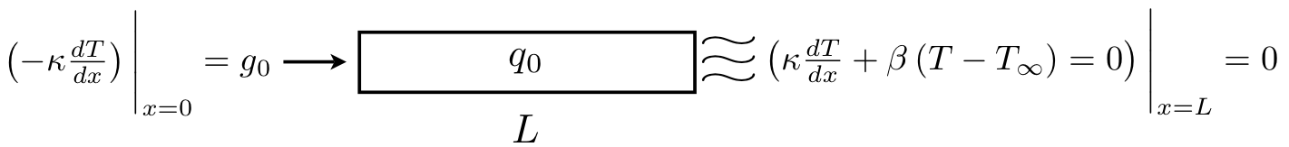
"## Example: Temperature Distribution in a Wall\n",
"\n",
"Consider a slab of length $L$ and constant thermal conductivity $\\kappa$ ($W\\cdot m^{-1}\\,^{\\circ}{C^{-1}})$\n",
"\n",
"
\n",
"\n",
"The balance of energy on the element requires\n",
"\n",
"$$ energy \\ in \\ + \\ energy \\ generated \\ = \\ change \\ in \\ internal \\ energy \\ + \\ energy \\ out $$\n",
"\n",
"or (referring to the above figure)\n",
"\n",
"$$ \\psi(x) + \\xi = \\Delta E + \\psi(x+dx) $$\n",
"\n",
"which can be written as\n",
"\n",
"$$ -\\kappa A \\frac{\\partial T}{{\\partial x}}\\Bigg|_{x=x}+qAdx=\\rho c_v A \\frac{\\partial T}{\\partial t}dx - \\kappa A \\frac{\\partial T}{{\\partial x}}\\Bigg|_{x=x+dx} $$\n",
"\n",
"where $q$ is the heat generation per unit volume. Using the first order Taylor series for $\\kappa A (\\partial{T}/\\partial{{ x}})|_{x=x+dx}$, we get\n",
"\n",
"$$ -\\kappa A \\frac{\\partial T}{{\\partial x}}+qAdx=\n",
"\\rho c_v A \\frac{\\partial T}{\\partial t}dx - \\left[ \n",
"\\kappa A \\frac{\\partial T}{{\\partial x}}+\n",
"\\frac{\\partial }{\\partial x}\\left( \\kappa A \\frac{\\partial T}{{\\partial x}} \\right) dx \n",
"\\right] \n",
"$$\n",
"\n",
"Finally, after some re-arranging, the heat equation becomes\n",
"\n",
"$$\n",
" \\frac{\\partial }{\\partial x}\\left(\\kappa A \\frac{\\partial T}{\\partial x}\\right) +Aq = \\rho c_v A\\frac{\\partial T}{\\partial t}\n",
"$$\n",
"\n",
"Considering only steady state conditions (meaning that there is no time dependence of the primary variable $T$) gives\n",
"\n",
"$$\n",
" \\frac{\\partial }{\\partial x}\\left(\\kappa A \\frac{\\partial T}{\\partial x}\\right) +Aq = 0\n",
"$$\n",
"\n",
"## Example: Temperature Distribution in a Wall\n",
"\n",
"Consider a slab of length $L$ and constant thermal conductivity $\\kappa$ ($W\\cdot m^{-1}\\,^{\\circ}{C^{-1}})$\n",
"\n",
" \n",
"\n",
"Suppose that energy at a uniform rate of $q_0$ ($Wm^{-3}$) is generated in the slab. We wish to determine the temperature distribution in the slab when the boundary surfaces of the wall are subject to the following boundary conditions\n",
"\n",
"$$ \\left( -\\kappa \\frac{dT}{dx}\\right)\\Bigg|_{x=0} = g_0 \\ (Wm^{-2}), \\quad \\left( \\kappa \\frac{dT}{dx}+\\beta (T-T_{\\infty})\\right)\\Bigg|_{x=L} = 0 $$\n",
"\n",
"In our example, the surface at $x=0$ is subjected to a uniform heat flux $g_0$ and heat is dissipated by convection into a fluid of temperature $T_{\\infty}$ at the surface at $x=L$. These boundary conditions give\n",
"\n",
"$$\n",
"Q_1^1= \\left( -\\kappa A \\frac{dT}{dx}\\right)\\Bigg|_{x=0} = Ag_0\n",
"$$\n",
"\n",
"and\n",
"\n",
"$$\n",
"Q_2^N = \\left( \\kappa A \\frac{dT}{dx} \\right)\\Bigg|_{x=L} = -\\beta A(T-T_{\\infty})\\Bigg|_{x=L}=-\\beta A\\left( u_N - T_{\\infty} \\right)\n",
"$$\n",
"\n",
"where $A$ is the cross-sectional area normal to the heat flow and $h$ is the heat transfer coefficient. For a two element mesh ($N=3$, $h_1=h_2=h=L/2$), the finite element equations are\n",
"\n",
"**Element 1**\n",
"\n",
"$$\n",
"\\frac{\\kappa A}{h}\n",
"\\left[ \\begin{array}{ccc} 1 & -1 & 0 \\newline -1 & 1 & 0 \\newline 0 & 0 & 0 \\end{array} \\right] \n",
"\\left\\{ \\begin{array}{c} u_1 \\newline u_2 \\newline u_3 \\end{array} \\right\\} \n",
"= \\frac{Aq_0h }{2}\n",
"\\left\\{ \\begin{array}{c} 1 \\newline 1 \\newline 0 \\end{array} \\right\\} \n",
"+ \\left\\{ \\begin{array}{c} Ag_0 \\newline 0 \\newline 0 \\end{array} \\right\\}\n",
"$$\n",
"\n",
"**Element 2**\n",
"\n",
"$$\n",
"\\frac{\\kappa A}{h}\n",
"\\left[ \\begin{array}{ccc} 0 & 0 & 0 \\newline 0 & 1 & -1 \\newline 0 & -1 & 1 \\end{array} \\right] \n",
"\\left\\{ \\begin{array}{c} u_1 \\newline u_2 \\newline u_3 \\end{array} \\right\\} = \n",
"\\frac{Aq_0h}{2}\n",
"\\left\\{ \\begin{array}{c} 0 \\newline 1 \\newline 1 \\end{array} \\right\\} + \n",
"\\left\\{ \\begin{array}{c} 0 \\newline 0 -A\\beta \\newline u_3 + A\\beta T_{\\infty} \\end{array} \\right\\}\n",
"$$\n",
"\n",
"**Global Equations**\n",
"\n",
"$$\n",
"\\frac{\\kappa A}{h}\n",
"\\left[ \\begin{array}{ccc} 1 & -1 & 0 \\newline -1 & 2 & -1 \\newline 0 & -1 & 1 \\end{array} \\right] \n",
"\\left\\{ \\begin{array}{c} u_1 \\newline u_2 \\newline u_3 \\end{array} \\right\\} \n",
"= \\frac{Aq_0h}{2}\\left\\{ \\begin{array}{c} 1 \\newline 2 \\newline 1 \\end{array} \\right\\} +\n",
"\\left\\{ \\begin{array}{c} Ag_0 \\newline 0 \\newline -A\\beta u_3 + A\\beta T_{\\infty} \\end{array} \\right\\}\n",
"$$\n",
"\n",
"or\n",
"\n",
"$$\n",
"\\frac{\\kappa A}{h}\n",
"\\left[ \\begin{array}{ccc} 1 & -1 & 0 \\newline -1 & 2 & -1 \\newline 0 & -1 & 1+\\beta h/\\kappa \\end{array} \\right] \n",
"\\left\\{ \\begin{array}{c} u_1 \\newline u_2 \\newline u_3 \\end{array} \\right\\} = \n",
"A \\left\\{ \\begin{array}{c} {\\frac{q_0h }{2}}+g_0 {{q_0h }} \\newline {\\frac{q_0h }{2}}+ \\beta T_{\\infty} \\end{array} \\right\\}\n",
"$$\n",
"\n",
"which can be solved for $u_1, \\ u_2$, and $u_3$\n",
"\n",
"$$\n",
"\\left\\{ \\begin{array}{c} u_1 \\newline u_2 \\newline u_3 \\end{array} \\right\\} =\n",
"\\frac{1}{\\kappa\\beta} \n",
"\\left[ \\begin {array}{c}\n",
"\\kappa\\left( 2q_0 h+ g_0\\right)+\\beta \\left( 2{h}^{2}q_0+2h g_0+\\kappa T \\right) \\newline \n",
"\\kappa \\left(2q_0h+g_0\\right) + \\beta \\left( 1.5 {h}^{2}q_0+ \\beta hg_0+\\kappa T \\right) \\newline \n",
"\\kappa(2 q_0h+g_0+\\beta T)\n",
"\\end {array} \\right]\n",
"$$"
]
},
{
"cell_type": "markdown",
"metadata": {},
"source": [
"# Fluid Mechanics[](#top)\n",
"\n",
"## Background\n",
"\n",
"The Navier-Stokes equation for the momentum of a fluid in the $x$-direction is\n",
"\n",
"$$\n",
"\\frac{\\partial }{\\partial x}\\left( 2\\mu \\frac{\\partial u}{\\partial x} - P \\right) + \\frac{\\partial }{\\partial y}\\left( \\mu \\left( \\frac{\\partial u}{\\partial y} + \\frac{\\partial v}{\\partial x} \\right) \\right) + f_x = \\rho\\left(\\frac{\\partial u}{\\partial t} + u\\frac{\\partial u}{\\partial x} + v\\frac{\\partial u}{\\partial y}\\right)\n",
"$$\n",
"\n",
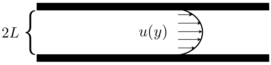
"Where $u$ and $v$ are the $x$ and $y$ components of the velocity, respectively, $P$ is the pressure, $f_x$ is the body force, $\\rho$ is the density, and $\\mu$ is the viscosity. For a fully developed laminar flow between two stationary parallel plates, separated by a distance $2L$, the velocity field is given by\n",
"\n",
"$$\n",
"u=u(y), \\ \\ \\ \\ v=0\n",
"$$\n",
"\n",
"With $P=P(x)$, $f_x=0$, and ${\\frac{\\partial u}{\\partial x}}=0$, the Navier-Stokes equation simplifies to\n",
"\n",
"$$\n",
"\\mu \\frac{d^2u}{d{y}^2}=\\frac{dP}{dx}\n",
"$$\n",
"\n",
"## Example: Flow Between Two Parallel Plates\n",
"\n",
"We now wish to determine the velocity distribution of the fluid between the two parallel plates for a given constant pressure gradient $dP/dx$. \n",
"\n",
"
\n",
"\n",
"Suppose that energy at a uniform rate of $q_0$ ($Wm^{-3}$) is generated in the slab. We wish to determine the temperature distribution in the slab when the boundary surfaces of the wall are subject to the following boundary conditions\n",
"\n",
"$$ \\left( -\\kappa \\frac{dT}{dx}\\right)\\Bigg|_{x=0} = g_0 \\ (Wm^{-2}), \\quad \\left( \\kappa \\frac{dT}{dx}+\\beta (T-T_{\\infty})\\right)\\Bigg|_{x=L} = 0 $$\n",
"\n",
"In our example, the surface at $x=0$ is subjected to a uniform heat flux $g_0$ and heat is dissipated by convection into a fluid of temperature $T_{\\infty}$ at the surface at $x=L$. These boundary conditions give\n",
"\n",
"$$\n",
"Q_1^1= \\left( -\\kappa A \\frac{dT}{dx}\\right)\\Bigg|_{x=0} = Ag_0\n",
"$$\n",
"\n",
"and\n",
"\n",
"$$\n",
"Q_2^N = \\left( \\kappa A \\frac{dT}{dx} \\right)\\Bigg|_{x=L} = -\\beta A(T-T_{\\infty})\\Bigg|_{x=L}=-\\beta A\\left( u_N - T_{\\infty} \\right)\n",
"$$\n",
"\n",
"where $A$ is the cross-sectional area normal to the heat flow and $h$ is the heat transfer coefficient. For a two element mesh ($N=3$, $h_1=h_2=h=L/2$), the finite element equations are\n",
"\n",
"**Element 1**\n",
"\n",
"$$\n",
"\\frac{\\kappa A}{h}\n",
"\\left[ \\begin{array}{ccc} 1 & -1 & 0 \\newline -1 & 1 & 0 \\newline 0 & 0 & 0 \\end{array} \\right] \n",
"\\left\\{ \\begin{array}{c} u_1 \\newline u_2 \\newline u_3 \\end{array} \\right\\} \n",
"= \\frac{Aq_0h }{2}\n",
"\\left\\{ \\begin{array}{c} 1 \\newline 1 \\newline 0 \\end{array} \\right\\} \n",
"+ \\left\\{ \\begin{array}{c} Ag_0 \\newline 0 \\newline 0 \\end{array} \\right\\}\n",
"$$\n",
"\n",
"**Element 2**\n",
"\n",
"$$\n",
"\\frac{\\kappa A}{h}\n",
"\\left[ \\begin{array}{ccc} 0 & 0 & 0 \\newline 0 & 1 & -1 \\newline 0 & -1 & 1 \\end{array} \\right] \n",
"\\left\\{ \\begin{array}{c} u_1 \\newline u_2 \\newline u_3 \\end{array} \\right\\} = \n",
"\\frac{Aq_0h}{2}\n",
"\\left\\{ \\begin{array}{c} 0 \\newline 1 \\newline 1 \\end{array} \\right\\} + \n",
"\\left\\{ \\begin{array}{c} 0 \\newline 0 -A\\beta \\newline u_3 + A\\beta T_{\\infty} \\end{array} \\right\\}\n",
"$$\n",
"\n",
"**Global Equations**\n",
"\n",
"$$\n",
"\\frac{\\kappa A}{h}\n",
"\\left[ \\begin{array}{ccc} 1 & -1 & 0 \\newline -1 & 2 & -1 \\newline 0 & -1 & 1 \\end{array} \\right] \n",
"\\left\\{ \\begin{array}{c} u_1 \\newline u_2 \\newline u_3 \\end{array} \\right\\} \n",
"= \\frac{Aq_0h}{2}\\left\\{ \\begin{array}{c} 1 \\newline 2 \\newline 1 \\end{array} \\right\\} +\n",
"\\left\\{ \\begin{array}{c} Ag_0 \\newline 0 \\newline -A\\beta u_3 + A\\beta T_{\\infty} \\end{array} \\right\\}\n",
"$$\n",
"\n",
"or\n",
"\n",
"$$\n",
"\\frac{\\kappa A}{h}\n",
"\\left[ \\begin{array}{ccc} 1 & -1 & 0 \\newline -1 & 2 & -1 \\newline 0 & -1 & 1+\\beta h/\\kappa \\end{array} \\right] \n",
"\\left\\{ \\begin{array}{c} u_1 \\newline u_2 \\newline u_3 \\end{array} \\right\\} = \n",
"A \\left\\{ \\begin{array}{c} {\\frac{q_0h }{2}}+g_0 {{q_0h }} \\newline {\\frac{q_0h }{2}}+ \\beta T_{\\infty} \\end{array} \\right\\}\n",
"$$\n",
"\n",
"which can be solved for $u_1, \\ u_2$, and $u_3$\n",
"\n",
"$$\n",
"\\left\\{ \\begin{array}{c} u_1 \\newline u_2 \\newline u_3 \\end{array} \\right\\} =\n",
"\\frac{1}{\\kappa\\beta} \n",
"\\left[ \\begin {array}{c}\n",
"\\kappa\\left( 2q_0 h+ g_0\\right)+\\beta \\left( 2{h}^{2}q_0+2h g_0+\\kappa T \\right) \\newline \n",
"\\kappa \\left(2q_0h+g_0\\right) + \\beta \\left( 1.5 {h}^{2}q_0+ \\beta hg_0+\\kappa T \\right) \\newline \n",
"\\kappa(2 q_0h+g_0+\\beta T)\n",
"\\end {array} \\right]\n",
"$$"
]
},
{
"cell_type": "markdown",
"metadata": {},
"source": [
"# Fluid Mechanics[](#top)\n",
"\n",
"## Background\n",
"\n",
"The Navier-Stokes equation for the momentum of a fluid in the $x$-direction is\n",
"\n",
"$$\n",
"\\frac{\\partial }{\\partial x}\\left( 2\\mu \\frac{\\partial u}{\\partial x} - P \\right) + \\frac{\\partial }{\\partial y}\\left( \\mu \\left( \\frac{\\partial u}{\\partial y} + \\frac{\\partial v}{\\partial x} \\right) \\right) + f_x = \\rho\\left(\\frac{\\partial u}{\\partial t} + u\\frac{\\partial u}{\\partial x} + v\\frac{\\partial u}{\\partial y}\\right)\n",
"$$\n",
"\n",
"Where $u$ and $v$ are the $x$ and $y$ components of the velocity, respectively, $P$ is the pressure, $f_x$ is the body force, $\\rho$ is the density, and $\\mu$ is the viscosity. For a fully developed laminar flow between two stationary parallel plates, separated by a distance $2L$, the velocity field is given by\n",
"\n",
"$$\n",
"u=u(y), \\ \\ \\ \\ v=0\n",
"$$\n",
"\n",
"With $P=P(x)$, $f_x=0$, and ${\\frac{\\partial u}{\\partial x}}=0$, the Navier-Stokes equation simplifies to\n",
"\n",
"$$\n",
"\\mu \\frac{d^2u}{d{y}^2}=\\frac{dP}{dx}\n",
"$$\n",
"\n",
"## Example: Flow Between Two Parallel Plates\n",
"\n",
"We now wish to determine the velocity distribution of the fluid between the two parallel plates for a given constant pressure gradient $dP/dx$. \n",
"\n",
" \n",
"\n",
"In this case, the DE is a special case of the same DE we have been solving all semester with $q={\\rm constant}=q_0$, $a=\\mu={\\rm constant}$, $c=0$, and $x=y$. Thus, the finite element model is\n",
"\n",
"$$\n",
"k^e_{ij}u_j^e = f_i^e + Q_i^e\n",
"$$\n",
"\n",
"with\n",
"\n",
"$$\n",
"Q_1^e=-\\left(\\mu\\frac{du}{dy}\\right)\\Bigg|_A, \\ \\ \\ \\ Q_2^e=\\left(\\mu\\frac{du}{dy}\\right)\\Bigg|_B\n",
"$$\n",
"\n",
"For a two element mesh of linear elements ($h=L$), we have\n",
"\n",
"$$\n",
"\\frac{\\mu}{h}\n",
"\\left[ \\begin{array}{ccc} 1 & -1 & 0 \\newline -1 & 2 & -1 \\newline 0 & -1 & 1 \\end{array} \\right] \n",
"\\left\\{ \\begin{array}{c} u_1 \\newline u_2 \\newline u_3 \\end{array} \\right\\} = \n",
"\\frac{q_0h}{2}\\left\\{ \\begin{array}{c} 1 \\newline 2 \\newline 1 \\end{array} \\right\\} + \n",
"\\left\\{ \\begin{array}{c} Q_1^1 \\newline Q_2^1+Q_1^2 \\newline Q_2^2 \\end{array} \\right\\}\n",
"$$\n",
"\n",
"Let us now consider the following boundary conditions, known as \"no-slip\" boundary conditions\n",
"\n",
"$$\n",
"u(-L)=u(L)=0\n",
"$$\n",
"\n",
"Then\n",
"\n",
"$$\n",
"\\frac{\\mu}{h}\\left[ \\begin{array}{ccc} 1 & -1 & 0 \\newline -1 & 2 & -1 \\newline 0 & -1 & 1 \\end{array} \\right] \n",
"\\left\\{ \\begin{array}{c} 0 \\newline u_2 \\newline 0 \\end{array} \\right\\} = \n",
"\\frac{q_0h}{2}\\left\\{ \\begin{array}{c} 1 \\newline 2 \\newline 1 \\end{array} \\right\\} +\n",
"\\left\\{ \\begin{array}{c} Q_1^1 \\newline 0 \\newline Q_2^2 \\end{array} \\right\\}\n",
"$$\n",
"\n",
"From which\n",
"\n",
"\n",
"$$\n",
"u_2=\\frac{q_0L^2}{2\\mu}\n",
"$$"
]
},
{
"cell_type": "markdown",
"metadata": {},
"source": [
"# Solid Mechanics[](#top)\n",
"\n",
"## Derivation of Governing DE for a Linear Elastic Bar\n",
"\n",
"Consider a bar of length L subjected to a body load and axial force as shown\n",
" \n",
"
\n",
"\n",
"In this case, the DE is a special case of the same DE we have been solving all semester with $q={\\rm constant}=q_0$, $a=\\mu={\\rm constant}$, $c=0$, and $x=y$. Thus, the finite element model is\n",
"\n",
"$$\n",
"k^e_{ij}u_j^e = f_i^e + Q_i^e\n",
"$$\n",
"\n",
"with\n",
"\n",
"$$\n",
"Q_1^e=-\\left(\\mu\\frac{du}{dy}\\right)\\Bigg|_A, \\ \\ \\ \\ Q_2^e=\\left(\\mu\\frac{du}{dy}\\right)\\Bigg|_B\n",
"$$\n",
"\n",
"For a two element mesh of linear elements ($h=L$), we have\n",
"\n",
"$$\n",
"\\frac{\\mu}{h}\n",
"\\left[ \\begin{array}{ccc} 1 & -1 & 0 \\newline -1 & 2 & -1 \\newline 0 & -1 & 1 \\end{array} \\right] \n",
"\\left\\{ \\begin{array}{c} u_1 \\newline u_2 \\newline u_3 \\end{array} \\right\\} = \n",
"\\frac{q_0h}{2}\\left\\{ \\begin{array}{c} 1 \\newline 2 \\newline 1 \\end{array} \\right\\} + \n",
"\\left\\{ \\begin{array}{c} Q_1^1 \\newline Q_2^1+Q_1^2 \\newline Q_2^2 \\end{array} \\right\\}\n",
"$$\n",
"\n",
"Let us now consider the following boundary conditions, known as \"no-slip\" boundary conditions\n",
"\n",
"$$\n",
"u(-L)=u(L)=0\n",
"$$\n",
"\n",
"Then\n",
"\n",
"$$\n",
"\\frac{\\mu}{h}\\left[ \\begin{array}{ccc} 1 & -1 & 0 \\newline -1 & 2 & -1 \\newline 0 & -1 & 1 \\end{array} \\right] \n",
"\\left\\{ \\begin{array}{c} 0 \\newline u_2 \\newline 0 \\end{array} \\right\\} = \n",
"\\frac{q_0h}{2}\\left\\{ \\begin{array}{c} 1 \\newline 2 \\newline 1 \\end{array} \\right\\} +\n",
"\\left\\{ \\begin{array}{c} Q_1^1 \\newline 0 \\newline Q_2^2 \\end{array} \\right\\}\n",
"$$\n",
"\n",
"From which\n",
"\n",
"\n",
"$$\n",
"u_2=\\frac{q_0L^2}{2\\mu}\n",
"$$"
]
},
{
"cell_type": "markdown",
"metadata": {},
"source": [
"# Solid Mechanics[](#top)\n",
"\n",
"## Derivation of Governing DE for a Linear Elastic Bar\n",
"\n",
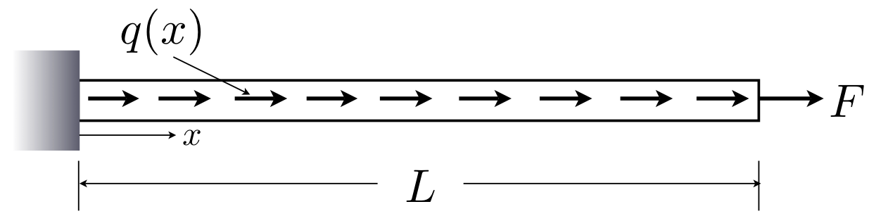
"Consider a bar of length L subjected to a body load and axial force as shown\n",
" \n",
" \n",
"\n",
"For the bar in equilibrium, the governing equation is\n",
"\n",
"$$\n",
"\\frac{d(A\\sigma)}{dx} + q = 0\n",
"$$\n",
"\n",
"Assuming linear elastic behavior, the constitutive model (stress-strain relationship) is\n",
"\n",
"$$\n",
"\\sigma = E\\epsilon\n",
"$$\n",
"\n",
"and the strain-displacement relationship is given by\n",
"\n",
"$$\n",
"\\epsilon = \\frac{du}{dx}\n",
"$$\n",
"\n",
"plugging the constitutive relationship and strain-displacement in to the governing DE gives\n",
"\n",
"$$\n",
"\\frac{d}{dx}\\left( AE\\frac{du}{dx}\\right) + q = 0\n",
"$$\n",
"\n",
"Two BCs are needed to solve a second order ODE. The first boundary condition, that at the wall, is simply the statement that the displacement at the wall is zero:\n",
"\n",
"$$\n",
"u(0) = 0\n",
"$$\n",
"\n",
"The second boundary condition, on the other hand, is more difficult to see. Often in texts, you will see the second boundary condition written as a \"force\" boundary condition:\n",
"\n",
"$$\n",
"AE\\frac{du}{dx}\\Bigg|_{x=L}=F\n",
"$$\n",
"\n",
"Where does this BC come from? Let us consider the end of the beam at $x=L$. At the beams end\n",
"\n",
"$$\n",
"A\\sigma=F\n",
"$$\n",
"\n",
"from the constitutive model and the stress strain relationship, this condition can be written as\n",
"\n",
"$$\n",
"A\\sigma=F=AE\\epsilon=AE\\frac{du}{dx}\\Bigg|_{x=L}=F\n",
"$$\n",
"\n",
"Thus, the governing differential equation for our bar problem is\n",
"\n",
"$$\n",
"\\frac{d}{dx}\\left( AE\\frac{du}{dx}\\right) + q = 0 \\ \\ {\\rm for} \\ x\\in(0,L)\n",
"$$\n",
"\n",
"subject to\n",
"\n",
"$$\n",
"u(0)=0, \\ \\ AE\\frac{du}{dx}\\Bigg|_{x=L}=F\n",
"$$\n",
"\n",
"Which is equivalent to the DE we've been investigating with $c(x)=0$, $u_0=0$, and $Q_0=F$."
]
},
{
"cell_type": "markdown",
"metadata": {},
"source": [
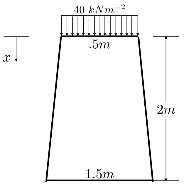
"## Example: Tapered Column\n",
"\n",
"Consider the problem of finding the displacements and stresses in a tapered steel ($\\gamma=78 \\ kNm^{-3}$, $E=200 GPa$) column with geometry and load shown, with a thickness of $t=.5m$.\n",
" \n",
"
\n",
"\n",
"For the bar in equilibrium, the governing equation is\n",
"\n",
"$$\n",
"\\frac{d(A\\sigma)}{dx} + q = 0\n",
"$$\n",
"\n",
"Assuming linear elastic behavior, the constitutive model (stress-strain relationship) is\n",
"\n",
"$$\n",
"\\sigma = E\\epsilon\n",
"$$\n",
"\n",
"and the strain-displacement relationship is given by\n",
"\n",
"$$\n",
"\\epsilon = \\frac{du}{dx}\n",
"$$\n",
"\n",
"plugging the constitutive relationship and strain-displacement in to the governing DE gives\n",
"\n",
"$$\n",
"\\frac{d}{dx}\\left( AE\\frac{du}{dx}\\right) + q = 0\n",
"$$\n",
"\n",
"Two BCs are needed to solve a second order ODE. The first boundary condition, that at the wall, is simply the statement that the displacement at the wall is zero:\n",
"\n",
"$$\n",
"u(0) = 0\n",
"$$\n",
"\n",
"The second boundary condition, on the other hand, is more difficult to see. Often in texts, you will see the second boundary condition written as a \"force\" boundary condition:\n",
"\n",
"$$\n",
"AE\\frac{du}{dx}\\Bigg|_{x=L}=F\n",
"$$\n",
"\n",
"Where does this BC come from? Let us consider the end of the beam at $x=L$. At the beams end\n",
"\n",
"$$\n",
"A\\sigma=F\n",
"$$\n",
"\n",
"from the constitutive model and the stress strain relationship, this condition can be written as\n",
"\n",
"$$\n",
"A\\sigma=F=AE\\epsilon=AE\\frac{du}{dx}\\Bigg|_{x=L}=F\n",
"$$\n",
"\n",
"Thus, the governing differential equation for our bar problem is\n",
"\n",
"$$\n",
"\\frac{d}{dx}\\left( AE\\frac{du}{dx}\\right) + q = 0 \\ \\ {\\rm for} \\ x\\in(0,L)\n",
"$$\n",
"\n",
"subject to\n",
"\n",
"$$\n",
"u(0)=0, \\ \\ AE\\frac{du}{dx}\\Bigg|_{x=L}=F\n",
"$$\n",
"\n",
"Which is equivalent to the DE we've been investigating with $c(x)=0$, $u_0=0$, and $Q_0=F$."
]
},
{
"cell_type": "markdown",
"metadata": {},
"source": [
"## Example: Tapered Column\n",
"\n",
"Consider the problem of finding the displacements and stresses in a tapered steel ($\\gamma=78 \\ kNm^{-3}$, $E=200 GPa$) column with geometry and load shown, with a thickness of $t=.5m$.\n",
" \n",
" \n",
"\n",
"Since we are going to approximate the problem in $1D$, we represent the distributed load at the top of the column as a point force\n",
"\n",
"$$ F=(0.5\\times 0.5)40 = 10kN $$\n",
"\n",
"The weight of the column is represented as a body force per unit length. The total force at any distance $x$ is equal to the weight of the column above that point. The weight at a distance $x$ is equal to the product of the volume of the body above $x$ and the specific weight of the column:\n",
"\n",
"$$ W(x)=0.5\\frac{1+0.5x}{2} x\\times 78 = 19.5(1+0.5x)x $$\n",
"\n",
"The body force per unit length is computed from\n",
"\n",
"$$ q=\\frac{dW}{dx}=19.5(1+x) $$\n",
"\n",
"The area $A(x)$ is given by\n",
"\n",
"\n",
"$$ A(x)=(0.5+0.5x)0.5=.25(1+x) $$\n",
"\n",
"\n",
"Thus,\n",
"\n",
"$$ \\frac{d}{dx}\\left( .25E(1+x)\\frac{du}{dx}\\right) + 19.5(1+x)=0 $$\n",
"\n",
"subject to the boundary conditions\n",
"\n",
"$$ \\left( .25E(1+x)\\frac{du}{dx}\\right)\\Bigg|_{x=0}=-10, \\ \\ \\ \\ u(2)=0 $$\n",
"\n",
"Again, the finite element model is given by\n",
"\n",
"\n",
"$$ k^e_{ij}u_j^e = f_i^e + Q_i^e $$\n",
"\n",
"with\n",
"\n",
"$$ Q_{x_1^{(e)}}^e=\\left( -.25E(1+x)\\frac{du}{dx}\\right)\\Bigg|_A, \\ \\ \\ \\ Q_{x_2^{(e)}}^e=\\left( .25E(1+x)\\frac{du}{dx}\\right)\\Bigg|_B $$\n",
"\n",
"For the linear element we have\n",
"\n",
"$$ k_{11}^e=\\int_{x_e}^{x_{e+1}}.25E(1+x)\\left( -\\frac{1}{h}\\right)^2\\,\\mathrm{d}{x}=\\frac{E}{4h_e}\\left( 1+.5\\left( x_e+x_{e+1}\\right) \\right) $$\n",
"\n",
"$$ f_{1}^e=\\int_{x_e}^{x_{e+1}}19.5(1+x)\\left( -\\frac{1}{h}\\right)\\,\\mathrm{d}{x}=19.5h_e\\left( .5 +.1667\\left( x_e+x_{e+1}\\right) \\right) $$\n",
"\n",
"Evaluating the other components gives\n",
"\n",
"$$ {\\boldsymbol{k}}^e=\\frac{E}{4h_e}\\left( 1+.5\\left( x_e+x_{e+1}\\right) \\right) \\left[ \\begin{array}{cc} 1 & -1 -1 & 1 \\end{array} \\right] $$\n",
"\n",
"$$ {\\boldsymbol{f}}^e=19.5\\frac{h_e}{2}\\left( \\left\\{\\begin{array}{c} 1 \\newline 1 \\end{array} \\right\\} + \\frac{1}{3}\\left\\{\\begin{array}{c}x_{e+1}+2x_e \\newline 2x_{e+1}+x_e \\end{array} \\right\\} \\right) $$\n",
"\n",
"Let us now consider a two element mesh with $h_1=h_2=1m$, then\n",
" \n",
"$$ {\\boldsymbol{k}}^{(1)}=\\frac{E}{4}\\left[\\begin{array}{cc}1.5 & -1.5 -1.5 & 1.5 \\end{array}\\right], \\ \\ \\ \\ {\\boldsymbol{f}}^{(1)}=\\frac{19.5}{2}\\left(\\left\\{\\begin{array}{c} 1 1\\end{array}\\right\\}+\\frac{1}{3}\\left\\{\\begin{array}{c} 1 2\\end{array}\\right\\}\\right)=\\left\\{\\begin{array}{c} 13 16.25\\end{array}\\right\\} $$\n",
"\n",
"$$ {\\boldsymbol{k}}^{(2)}=\\frac{E}{4}\\left[\\begin{array}{cc}2.5 & -2.5 \\newline -2.5 & 2.5 \\end{array}\\right], \\ \\ \\ \\ {\\boldsymbol{f}}^{(2)}=\\frac{19.5}{2}\\left(\\left\\{\\begin{array}{c} 1\\newline1\\end{array}\\right\\}+\\frac{1}{3}\\left\\{\\begin{array}{c} 4\\newline5\\end{array}\\right\\}\\right)=\\left\\{\\begin{array}{c} 22.75\\newline26\\end{array}\\right\\} $$\n",
"\n",
"The global equations are\n",
"\n",
"$$ E\\left[ \n",
"\\begin{array}{ccc} \n",
"0.375 & -0.375 & 0.000 \\newline \n",
"-0.375 & 1.000 & -0.625 \\newline \n",
"0.000 & -0.625 & 0.625 \\end{array}\n",
"\\right]\\left\\{\\begin{array}{c}\n",
"u_1 \\newline u_2 \\newline u_3 \\end{array} \\right\\}\n",
"= \\left\\{ \\begin{array}{c} \n",
"13 \\newline 39 \\newline 26 \\end{array} \\right\\} + \n",
"\\left\\{ \\begin{array}{c} Q_1^1 \\newline Q_2^1+Q_1^2 \\newline Q_2^2 \\end{array} \\right\\} $$\n",
"\n",
"Boundary conditions:\n",
"\n",
"$$ u_3=0, \\quad Q_1^1=\\left(-EA\\frac{du}{dx}\\right)\\Bigg|_{x=0}=-(-10)=10 $$\n",
"\n",
"Equilibrium condition:\n",
"\n",
"$$ Q_2^1+Q_1^2=0 $$\n",
"\n",
"Inserting the boundary and equilibrium conditions into the global equations gives a system of three equations for the three unknowns $u_2, \\ u_2, \\ Q_2^2$."
]
},
{
"cell_type": "markdown",
"metadata": {},
"source": [
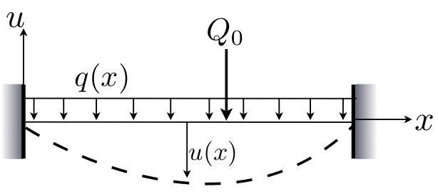
"# Example: Point Loads on the Interior of Elements\n",
"\n",
"Let us consider the problem of finding the deflection of a wire with tension $T$ and due to the distributed load $q(x)$, with a point source $Q_0$ at $\\hat x=5L/8$ as shown below\n",
"\n",
"
\n",
"\n",
"Since we are going to approximate the problem in $1D$, we represent the distributed load at the top of the column as a point force\n",
"\n",
"$$ F=(0.5\\times 0.5)40 = 10kN $$\n",
"\n",
"The weight of the column is represented as a body force per unit length. The total force at any distance $x$ is equal to the weight of the column above that point. The weight at a distance $x$ is equal to the product of the volume of the body above $x$ and the specific weight of the column:\n",
"\n",
"$$ W(x)=0.5\\frac{1+0.5x}{2} x\\times 78 = 19.5(1+0.5x)x $$\n",
"\n",
"The body force per unit length is computed from\n",
"\n",
"$$ q=\\frac{dW}{dx}=19.5(1+x) $$\n",
"\n",
"The area $A(x)$ is given by\n",
"\n",
"\n",
"$$ A(x)=(0.5+0.5x)0.5=.25(1+x) $$\n",
"\n",
"\n",
"Thus,\n",
"\n",
"$$ \\frac{d}{dx}\\left( .25E(1+x)\\frac{du}{dx}\\right) + 19.5(1+x)=0 $$\n",
"\n",
"subject to the boundary conditions\n",
"\n",
"$$ \\left( .25E(1+x)\\frac{du}{dx}\\right)\\Bigg|_{x=0}=-10, \\ \\ \\ \\ u(2)=0 $$\n",
"\n",
"Again, the finite element model is given by\n",
"\n",
"\n",
"$$ k^e_{ij}u_j^e = f_i^e + Q_i^e $$\n",
"\n",
"with\n",
"\n",
"$$ Q_{x_1^{(e)}}^e=\\left( -.25E(1+x)\\frac{du}{dx}\\right)\\Bigg|_A, \\ \\ \\ \\ Q_{x_2^{(e)}}^e=\\left( .25E(1+x)\\frac{du}{dx}\\right)\\Bigg|_B $$\n",
"\n",
"For the linear element we have\n",
"\n",
"$$ k_{11}^e=\\int_{x_e}^{x_{e+1}}.25E(1+x)\\left( -\\frac{1}{h}\\right)^2\\,\\mathrm{d}{x}=\\frac{E}{4h_e}\\left( 1+.5\\left( x_e+x_{e+1}\\right) \\right) $$\n",
"\n",
"$$ f_{1}^e=\\int_{x_e}^{x_{e+1}}19.5(1+x)\\left( -\\frac{1}{h}\\right)\\,\\mathrm{d}{x}=19.5h_e\\left( .5 +.1667\\left( x_e+x_{e+1}\\right) \\right) $$\n",
"\n",
"Evaluating the other components gives\n",
"\n",
"$$ {\\boldsymbol{k}}^e=\\frac{E}{4h_e}\\left( 1+.5\\left( x_e+x_{e+1}\\right) \\right) \\left[ \\begin{array}{cc} 1 & -1 -1 & 1 \\end{array} \\right] $$\n",
"\n",
"$$ {\\boldsymbol{f}}^e=19.5\\frac{h_e}{2}\\left( \\left\\{\\begin{array}{c} 1 \\newline 1 \\end{array} \\right\\} + \\frac{1}{3}\\left\\{\\begin{array}{c}x_{e+1}+2x_e \\newline 2x_{e+1}+x_e \\end{array} \\right\\} \\right) $$\n",
"\n",
"Let us now consider a two element mesh with $h_1=h_2=1m$, then\n",
" \n",
"$$ {\\boldsymbol{k}}^{(1)}=\\frac{E}{4}\\left[\\begin{array}{cc}1.5 & -1.5 -1.5 & 1.5 \\end{array}\\right], \\ \\ \\ \\ {\\boldsymbol{f}}^{(1)}=\\frac{19.5}{2}\\left(\\left\\{\\begin{array}{c} 1 1\\end{array}\\right\\}+\\frac{1}{3}\\left\\{\\begin{array}{c} 1 2\\end{array}\\right\\}\\right)=\\left\\{\\begin{array}{c} 13 16.25\\end{array}\\right\\} $$\n",
"\n",
"$$ {\\boldsymbol{k}}^{(2)}=\\frac{E}{4}\\left[\\begin{array}{cc}2.5 & -2.5 \\newline -2.5 & 2.5 \\end{array}\\right], \\ \\ \\ \\ {\\boldsymbol{f}}^{(2)}=\\frac{19.5}{2}\\left(\\left\\{\\begin{array}{c} 1\\newline1\\end{array}\\right\\}+\\frac{1}{3}\\left\\{\\begin{array}{c} 4\\newline5\\end{array}\\right\\}\\right)=\\left\\{\\begin{array}{c} 22.75\\newline26\\end{array}\\right\\} $$\n",
"\n",
"The global equations are\n",
"\n",
"$$ E\\left[ \n",
"\\begin{array}{ccc} \n",
"0.375 & -0.375 & 0.000 \\newline \n",
"-0.375 & 1.000 & -0.625 \\newline \n",
"0.000 & -0.625 & 0.625 \\end{array}\n",
"\\right]\\left\\{\\begin{array}{c}\n",
"u_1 \\newline u_2 \\newline u_3 \\end{array} \\right\\}\n",
"= \\left\\{ \\begin{array}{c} \n",
"13 \\newline 39 \\newline 26 \\end{array} \\right\\} + \n",
"\\left\\{ \\begin{array}{c} Q_1^1 \\newline Q_2^1+Q_1^2 \\newline Q_2^2 \\end{array} \\right\\} $$\n",
"\n",
"Boundary conditions:\n",
"\n",
"$$ u_3=0, \\quad Q_1^1=\\left(-EA\\frac{du}{dx}\\right)\\Bigg|_{x=0}=-(-10)=10 $$\n",
"\n",
"Equilibrium condition:\n",
"\n",
"$$ Q_2^1+Q_1^2=0 $$\n",
"\n",
"Inserting the boundary and equilibrium conditions into the global equations gives a system of three equations for the three unknowns $u_2, \\ u_2, \\ Q_2^2$."
]
},
{
"cell_type": "markdown",
"metadata": {},
"source": [
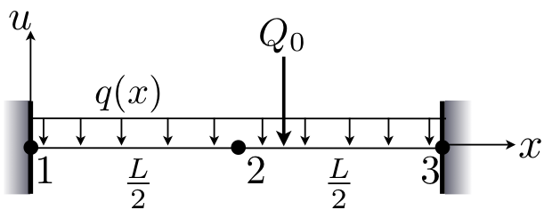
"# Example: Point Loads on the Interior of Elements\n",
"\n",
"Let us consider the problem of finding the deflection of a wire with tension $T$ and due to the distributed load $q(x)$, with a point source $Q_0$ at $\\hat x=5L/8$ as shown below\n",
"\n",
" \n",
"\n",
"The deflection of the wire can be modeled by a special case of the same $2^{\\rm nd}$ order DE we have been studying:\n",
"\n",
"$$\n",
" \\frac{d}{dx}\\left( a(x) \\frac{du(x)}{dx} \\right) - c(x)u(x)+q(x) = 0 \\ \\ {\\rm for} \\ x\\in(0,L)\n",
"$$\n",
"\n",
"with $c(x)=0$:\n",
"\n",
"$$\n",
" T \\frac{d^2u(x)}{d{x}^2} + q(x) = 0 \\ \\ {\\rm for} \\ x\\in(0,L)\n",
"$$\n",
"\n",
"Recall the weak form\n",
"\n",
"$$\n",
" \\int_0^L w'(x)u'(x) \\,\\mathrm{d}{x} - \\frac{1}{T}\\int_0^Lw(x)q(x)\\,\\mathrm{d}{x}=w(x)u'(x)\\Bigg|_0^L\n",
"$$\n",
"\n",
"where $w(x)$ is the weight function. Suppose now we choose a two element mesh to represent the problem domain with $h_1=h_2=L/2$\n",
"\n",
"
\n",
"\n",
"The deflection of the wire can be modeled by a special case of the same $2^{\\rm nd}$ order DE we have been studying:\n",
"\n",
"$$\n",
" \\frac{d}{dx}\\left( a(x) \\frac{du(x)}{dx} \\right) - c(x)u(x)+q(x) = 0 \\ \\ {\\rm for} \\ x\\in(0,L)\n",
"$$\n",
"\n",
"with $c(x)=0$:\n",
"\n",
"$$\n",
" T \\frac{d^2u(x)}{d{x}^2} + q(x) = 0 \\ \\ {\\rm for} \\ x\\in(0,L)\n",
"$$\n",
"\n",
"Recall the weak form\n",
"\n",
"$$\n",
" \\int_0^L w'(x)u'(x) \\,\\mathrm{d}{x} - \\frac{1}{T}\\int_0^Lw(x)q(x)\\,\\mathrm{d}{x}=w(x)u'(x)\\Bigg|_0^L\n",
"$$\n",
"\n",
"where $w(x)$ is the weight function. Suppose now we choose a two element mesh to represent the problem domain with $h_1=h_2=L/2$\n",
"\n",
" \n",
"\n",
"The point source is now on the interior of element 2. Thus far in our finite element analysis, point sources at the nodes are included in the finite element model via the balance of sources at the nodes and we have not considered point sources on the interior of elements. If a point source does not occur at a node it is possible to ''distribute'' it to the element nodes.\n",
"Let $Q_0$ denote a point source at the point $x_0$, $x_e\\leq x_0 \\leq x_{e+1}$. The point source $Q_0$ can be represented as a ``function'' by\n",
"\n",
"$$ Q(x)=Q_0\\delta(x-x_0) $$\n",
"\n",
" \n",
"Where the Dirac delta function $\\delta(x-x_0)$, is defined by:\n",
" \n",
"$$\n",
"\\int_{-\\infty}^{\\infty}y(x)\\delta(x-x_0)\\,\\mathrm{d}{x}=y(x_0)\n",
"$$\n",
"\n",
"The contribution of the function $q(x)$ to the nodes of the element $\\Omega^e=(x_e,x_{e+1})$ is computed from\n",
" \n",
"$$\n",
"\\bar{Q}_i^e=\\int_{-\\infty}^{\\infty}Q(x)\\phi_i^e(x)\\,\\mathrm{d}{x}\n",
"$$\n",
"\n",
"which, because of the compact support of the basis functions, can be written\n",
" \n",
"$$\n",
"\\bar{Q}_i^e=\\int_{x_e}^{x_{e+1}}Q(x)\\phi_i^e(x)\\,\\mathrm{d}{x} = \\int_{x_e}^{x_{e+1}}Q_0\\delta(x-x_0)\\phi_i^e(x)\\,\\mathrm{d}{x}=Q_0\\phi_i^e(x_0)\n",
"$$\n",
"\n",
"where $\\phi_i^e$ are the interpolation functions of the element $\\Omega^e$. Thus, the point source $Q_0$ is distributed to the element node $i$ by the value $Q_0\\phi_i^e(x_0)$. This holds for any element, regardless of the degree/type of interpolation. For the linear Lagrange interpolation functions in 1D, we get\n",
" \n",
"$$\n",
"{\\bar{Q}}_1^e=Q_0\\frac{x_{e+1}-x_0}{h_e}=\\alpha Q_0, \\quad \\bar{Q}_2^e=Q_0\\frac{x_{0}-x_e}{h_e}=(1-\\alpha)Q_0\n",
"$$\n",
"\n",
"where $\\alpha=(x_{e+1}-x_0)/h_e$ is the ratio of the distance between node 2 and the source to the length of the element. Now, returning to our example, the finite element equations for the transverse deflection of the wire are:\n",
" \n",
"$$\n",
"T\\sum_{e=1}^2k_{ij}^eu_j^e=f_i^e+Q_i^e + \\bar{Q}_i^e\n",
"$$\n",
"\n",
"The point source is included using:\n",
" \n",
"$$\n",
"\\bar{Q}_1^2=2Q_0\\frac{L-\\frac{5L}{8}}{L}=\\frac{3Q_0}{4}, \\quad \\bar{Q}_2^2=2Q_0\\frac{\\frac{5L}{8}-\\frac{1L}{2}}{L}=\\frac{Q_0}{4}\n",
"$$\n",
"\n",
"Substitution gives\n",
" \n",
"$$\n",
"T\\sum_{e=1}^2k_{ij}^eu_j^e=f_i^e+Q_i^e + \\frac{Q_0}{4} \\begin{pmatrix} 0 \\newline 3 \\newline 1 \\end{pmatrix}\n",
"$$\n",
"\n",
"$$\n",
"\\Rightarrow\\frac{2T}{L}\n",
"\\begin{pmatrix} \n",
"1 & -1 & 0 \\newline \n",
"-1 & 2 & -1 \\newline\n",
"0 & -1 & 1 \\end{pmatrix}\n",
"\\begin{pmatrix} u_1 \\newline u_2 \\newline u_3 \\end{pmatrix}\n",
"=\\frac{qL}{4}\\begin{pmatrix}1 2 1\\end{pmatrix} \n",
"+ \n",
"\\begin{pmatrix} \n",
"Q_1^1 \\newline 0 \\newline Q_2^2 \n",
"\\end{pmatrix}\n",
"+\n",
"\\frac{Q_0}{4} \\begin{pmatrix} 0 \\newline 3 \\newline 1 \\end{pmatrix}\n",
"$$\n",
"\n",
"Applying the boundary conditions:\n",
" \n",
"$$\n",
"u(0)=u_1=0, \\qquad u(L)=u_3=0\n",
"$$\n",
"\n",
"gives\n",
" \n",
"$$\n",
"\\Rightarrow\\frac{2T}{L}\n",
"\\begin{pmatrix} \n",
"1 & -1 & 0 \\newline\n",
"-1 & 2 & -1 \\newline\n",
"0 & -1 & 1 \n",
"\\end{pmatrix}\n",
"\\begin{pmatrix} 0 \\newline u_2 \\newline 0 \n",
"\\end{pmatrix} = \\frac{1}{4}\\begin{pmatrix} qL + 4Q_1^1 \\newline 2qL+3Q_0 \\newline qL+4Q_2^2+Q_0 \\end{pmatrix}\n",
"$$\n",
"\n",
"From which\n",
" \n",
"$$\n",
"u_2 = L\\frac{2qL+3Q_0}{16T}\n",
"$$\n",
"\n",
"then\n",
" \n",
"$$\n",
"Q_1^1=-\\frac{1}{4}\\left(\\frac{8T}{L}u_2+qL\\right)=-\\frac{qL}{2}-\\frac{3Q_0}{8}\n",
"$$\n",
"\n",
"$$\n",
"Q_2^2=-\\frac{1}{4}\\left(\\frac{8T}{L}u_2+qL+Q_0\\right)=-\\frac{qL}{2}-\\frac{5Q_0}{8}\n",
"$$\n",
"\n",
"We can verify that we solved the equations correctly by comparing our result for the reactions $Q_i^e$ with the equilibrium requirement:\n",
" \n",
"$$\n",
"\\sum F_y = 0\n",
"$$\n",
"\n",
"$$\n",
"\\Rightarrow \\sum F_y = qL+Q_0 - Q_1^1-Q_2^2 = qL+Q_0 -\\frac{3Q_0}{8}-\\frac{qL}{2}-\\frac{qL}{2}-\\frac{5Q_0}{8}=0\n",
"$$\n",
"\n",
"Sure enough, equilibrium is satisfied and we can have confidence in our solution.\n",
"\n",
"We have seen in this previous example how to handle point loads that lie on the interior of an element. We saw that including these point loads involves an increase of work and a decrease in the quality of our model (i.e., the point load was distributed among two nodes). In practice, it is easier and more accurate to place a node at the location of a point force."
]
},
{
"cell_type": "markdown",
"metadata": {},
"source": [
"# Example: Axisymmetry\n",
"\n",
"Consider a long solid cylinder of radius $R_0$ in which energy is generated at a constant rate $q_0 \\ (Wm^{-3})$. The boundary surface at $r=R_0$ is maintained at a constant temperature $T_0$. We wish to calculate the temperature distribution $T(r)$ and heat flux $q(r)=-kdT/dr$ (or heat $Q=-AkdT/dr$), shown below\n",
"\n",
"
\n",
"\n",
"The point source is now on the interior of element 2. Thus far in our finite element analysis, point sources at the nodes are included in the finite element model via the balance of sources at the nodes and we have not considered point sources on the interior of elements. If a point source does not occur at a node it is possible to ''distribute'' it to the element nodes.\n",
"Let $Q_0$ denote a point source at the point $x_0$, $x_e\\leq x_0 \\leq x_{e+1}$. The point source $Q_0$ can be represented as a ``function'' by\n",
"\n",
"$$ Q(x)=Q_0\\delta(x-x_0) $$\n",
"\n",
" \n",
"Where the Dirac delta function $\\delta(x-x_0)$, is defined by:\n",
" \n",
"$$\n",
"\\int_{-\\infty}^{\\infty}y(x)\\delta(x-x_0)\\,\\mathrm{d}{x}=y(x_0)\n",
"$$\n",
"\n",
"The contribution of the function $q(x)$ to the nodes of the element $\\Omega^e=(x_e,x_{e+1})$ is computed from\n",
" \n",
"$$\n",
"\\bar{Q}_i^e=\\int_{-\\infty}^{\\infty}Q(x)\\phi_i^e(x)\\,\\mathrm{d}{x}\n",
"$$\n",
"\n",
"which, because of the compact support of the basis functions, can be written\n",
" \n",
"$$\n",
"\\bar{Q}_i^e=\\int_{x_e}^{x_{e+1}}Q(x)\\phi_i^e(x)\\,\\mathrm{d}{x} = \\int_{x_e}^{x_{e+1}}Q_0\\delta(x-x_0)\\phi_i^e(x)\\,\\mathrm{d}{x}=Q_0\\phi_i^e(x_0)\n",
"$$\n",
"\n",
"where $\\phi_i^e$ are the interpolation functions of the element $\\Omega^e$. Thus, the point source $Q_0$ is distributed to the element node $i$ by the value $Q_0\\phi_i^e(x_0)$. This holds for any element, regardless of the degree/type of interpolation. For the linear Lagrange interpolation functions in 1D, we get\n",
" \n",
"$$\n",
"{\\bar{Q}}_1^e=Q_0\\frac{x_{e+1}-x_0}{h_e}=\\alpha Q_0, \\quad \\bar{Q}_2^e=Q_0\\frac{x_{0}-x_e}{h_e}=(1-\\alpha)Q_0\n",
"$$\n",
"\n",
"where $\\alpha=(x_{e+1}-x_0)/h_e$ is the ratio of the distance between node 2 and the source to the length of the element. Now, returning to our example, the finite element equations for the transverse deflection of the wire are:\n",
" \n",
"$$\n",
"T\\sum_{e=1}^2k_{ij}^eu_j^e=f_i^e+Q_i^e + \\bar{Q}_i^e\n",
"$$\n",
"\n",
"The point source is included using:\n",
" \n",
"$$\n",
"\\bar{Q}_1^2=2Q_0\\frac{L-\\frac{5L}{8}}{L}=\\frac{3Q_0}{4}, \\quad \\bar{Q}_2^2=2Q_0\\frac{\\frac{5L}{8}-\\frac{1L}{2}}{L}=\\frac{Q_0}{4}\n",
"$$\n",
"\n",
"Substitution gives\n",
" \n",
"$$\n",
"T\\sum_{e=1}^2k_{ij}^eu_j^e=f_i^e+Q_i^e + \\frac{Q_0}{4} \\begin{pmatrix} 0 \\newline 3 \\newline 1 \\end{pmatrix}\n",
"$$\n",
"\n",
"$$\n",
"\\Rightarrow\\frac{2T}{L}\n",
"\\begin{pmatrix} \n",
"1 & -1 & 0 \\newline \n",
"-1 & 2 & -1 \\newline\n",
"0 & -1 & 1 \\end{pmatrix}\n",
"\\begin{pmatrix} u_1 \\newline u_2 \\newline u_3 \\end{pmatrix}\n",
"=\\frac{qL}{4}\\begin{pmatrix}1 2 1\\end{pmatrix} \n",
"+ \n",
"\\begin{pmatrix} \n",
"Q_1^1 \\newline 0 \\newline Q_2^2 \n",
"\\end{pmatrix}\n",
"+\n",
"\\frac{Q_0}{4} \\begin{pmatrix} 0 \\newline 3 \\newline 1 \\end{pmatrix}\n",
"$$\n",
"\n",
"Applying the boundary conditions:\n",
" \n",
"$$\n",
"u(0)=u_1=0, \\qquad u(L)=u_3=0\n",
"$$\n",
"\n",
"gives\n",
" \n",
"$$\n",
"\\Rightarrow\\frac{2T}{L}\n",
"\\begin{pmatrix} \n",
"1 & -1 & 0 \\newline\n",
"-1 & 2 & -1 \\newline\n",
"0 & -1 & 1 \n",
"\\end{pmatrix}\n",
"\\begin{pmatrix} 0 \\newline u_2 \\newline 0 \n",
"\\end{pmatrix} = \\frac{1}{4}\\begin{pmatrix} qL + 4Q_1^1 \\newline 2qL+3Q_0 \\newline qL+4Q_2^2+Q_0 \\end{pmatrix}\n",
"$$\n",
"\n",
"From which\n",
" \n",
"$$\n",
"u_2 = L\\frac{2qL+3Q_0}{16T}\n",
"$$\n",
"\n",
"then\n",
" \n",
"$$\n",
"Q_1^1=-\\frac{1}{4}\\left(\\frac{8T}{L}u_2+qL\\right)=-\\frac{qL}{2}-\\frac{3Q_0}{8}\n",
"$$\n",
"\n",
"$$\n",
"Q_2^2=-\\frac{1}{4}\\left(\\frac{8T}{L}u_2+qL+Q_0\\right)=-\\frac{qL}{2}-\\frac{5Q_0}{8}\n",
"$$\n",
"\n",
"We can verify that we solved the equations correctly by comparing our result for the reactions $Q_i^e$ with the equilibrium requirement:\n",
" \n",
"$$\n",
"\\sum F_y = 0\n",
"$$\n",
"\n",
"$$\n",
"\\Rightarrow \\sum F_y = qL+Q_0 - Q_1^1-Q_2^2 = qL+Q_0 -\\frac{3Q_0}{8}-\\frac{qL}{2}-\\frac{qL}{2}-\\frac{5Q_0}{8}=0\n",
"$$\n",
"\n",
"Sure enough, equilibrium is satisfied and we can have confidence in our solution.\n",
"\n",
"We have seen in this previous example how to handle point loads that lie on the interior of an element. We saw that including these point loads involves an increase of work and a decrease in the quality of our model (i.e., the point load was distributed among two nodes). In practice, it is easier and more accurate to place a node at the location of a point force."
]
},
{
"cell_type": "markdown",
"metadata": {},
"source": [
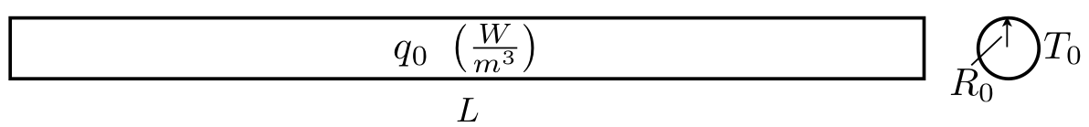
"# Example: Axisymmetry\n",
"\n",
"Consider a long solid cylinder of radius $R_0$ in which energy is generated at a constant rate $q_0 \\ (Wm^{-3})$. The boundary surface at $r=R_0$ is maintained at a constant temperature $T_0$. We wish to calculate the temperature distribution $T(r)$ and heat flux $q(r)=-kdT/dr$ (or heat $Q=-AkdT/dr$), shown below\n",
"\n",
" \n",
"\n",
"In general, this type of problem is 3D and requires solving a PDE in $x,y,z$. However, if the energy generation, boundary conditions, and material properties are all only functions of the radius $r$ and the temperature distribution along the length of the cylinder is approximately the approximately the same, it is sufficient to consider any cross section away from the ends. Or, the problem is reduced from 3D in $x,y,z$ to 2D in $r,\\theta$. Since the problem data are independent of the circumferential direction $\\theta$, the temperature distribution along any radius is the same, thereby reducing the 2D problem to a 1D one.\n",
"\n",
"Problems of this sort are described by the DE\n",
" \n",
"$$\n",
" -\\frac{1}{r}\\frac{d}{dr}\\left( a(r)\\frac{du}{dr}\\right)-q(r)=0, \\qquad r\\in(0,R_0)\n",
"$$\n",
"\n",
"which can be found by performing the coordinate change $x=r\\cos\\theta$, $y=r\\sin\\theta$, $x^2+y^2=r^2$, and $\\tan\\theta=x/y$.\n",
"\n",
"We now develop the weak form of the axisymmetric equation as we have done before, namely, we multiply by a weight function $w(r)$ and integrate over the problem domain. However, this time we must integrate over the volume of the cylinder of unit length:\n",
" \n",
"$$\n",
"\\int_V\\left( -\\frac{1}{r}\\frac{d}{dr}\\left( a\\frac{du}{dr}\\right)-q \\right) w \\ rdrd\\theta dz=0\n",
"$$\n",
"\n",
"$$\n",
"=\\int_0^1\\int_0^{2\\pi}\\int_{r_1}^{r_2}\\left( -\\frac{1}{r}\\frac{d}{dr}\\left( a\\frac{du}{dr}\\right)-q \\right) w \\ rdrd\\theta dz=0\n",
"$$\n",
"\n",
"where $(r_1,r_2)$ is the domain of the element along the radial direction. Next we integrate in $\\theta$ and $z$\n",
" \n",
"$$\n",
"=2\\pi\\int_{r_1}^{r_2}\\left( -\\frac{1}{r}\\frac{d}{dr}\\left( a\\frac{du}{dr}\\right)-q \\right) w \\ rdr=0\n",
"$$\n",
"\n",
"and integrate by parts\n",
" \n",
"$$\n",
"=2\\pi\\int_{r_1}^{r_2} a\\frac{dw}{dr}\\frac{du}{dr}-rqw \\ dr -\\left( w2\\pi a\\frac{du}{dr}\\right)_{r_1}^{r_2}=0\n",
"$$\n",
"\n",
"$$\n",
"=2\\pi\\int_{r_1}^{r_2} a\\frac{dw}{dr}\\frac{du}{dr}-rqw \\ dr -w(r_1)Q_1^e-w(r_2)Q_2^e=0\n",
"$$\n",
"\n",
"where\n",
" \n",
"$$\n",
"Q_1^e=-2\\pi\\left( a\\frac{du}{dr}\\right)\\Bigg|_{r_1}, \\qquad Q_2^e=2\\pi\\left( a\\frac{du}{dr}\\right)\\Bigg|_{r_2}\n",
"$$\n",
"\n",
"The finite element model is obtained by substituting the approximation\n",
" \n",
"$$\n",
"u(r)\\approx U_N(r)=\\sum_{j=1}^{n-1}u_j\\phi_j^e(r)\n",
"$$\n",
"\n",
"to get\n",
" \n",
"$$\n",
"{\\boldsymbol{k}}^e{\\boldsymbol{u}}^e={\\boldsymbol{f}}^e+{\\boldsymbol{Q}}^e\n",
"$$\n",
"\n",
"where\n",
" \n",
"$$\n",
"k_{ij}^e=2\\pi\\int_{r_1}^{r_2}a\\frac{d\\phi_i^e}{dr}\\frac{d\\phi_j}{dr}dr, \\qquad f_i^e=2\\pi\\int_{r_1}^{r_2}\\phi_i^eqrdr\n",
"$$\n",
"\n",
"where $\\phi_i^e$ are the interpolation functions expressed in terms of the radial coordinate $r$. In the case of a linear interpolation function, $\\phi_i^e$ takes the form:\n",
" \n",
"$$\n",
"\\phi_1^e=\\frac{r_2-r}{h_e}, \\qquad \\phi_2^e=\\frac{r-r_1}{h_e}\n",
"$$\n",
"\n",
"Substitution gives\n",
" \n",
"$$\n",
"{\\boldsymbol{k}}^e=\\frac{2\\pi a}{h_e}\\left( r_1 + \\frac{1}{2} h_e\\right)\n",
"\\begin{pmatrix} 1 & -1 \\newline -1 & 1 \\end{pmatrix}, \\quad \n",
"{\\boldsymbol{f}}^e=\\frac{2\\pi q_eh_e}{6}\\begin{pmatrix} 3r_1+h_e \\\\ 3r_1 + 2h_e \\end{pmatrix}\n",
"$$\n",
"\n",
"Let us now return to our example problem. The boundary conditions are\n",
" \n",
"$$\n",
"T(R_0)=T_0, \\qquad \\left( 2\\pi kr\\frac{dT}{dr}\\right)\\Bigg|_{r=0}=0\n",
"$$\n",
"\n",
"The zero-flux boundary condition at $r=0$ follows from the fact that the domain is radially symmetric about $r=0$. If, however, the cylinder were hollow, we could specify a temperature or heat flux at the inner radius.\n",
" \n",
"Letting $a=kr$, the finite element model of the governing equation is given by\n",
" \n",
"$$\n",
"{\\boldsymbol{k}}^e{\\boldsymbol{u}}^e={\\boldsymbol{f}}^e+{\\boldsymbol{Q}}^e\n",
"$$\n",
"\n",
"where\n",
" \n",
"$$\n",
"k_{ij}^e=2\\pi\\int_{r_1}^{r_2}kr\\frac{d\\phi_i^e}{dr}\\frac{d\\phi_j}{dr}dr, \\quad f_i^e=2\\pi\\int_{r_1}^{r_2}\\phi_i^eq_0rdr\n",
"$$\n",
" \n",
"$$\n",
"Q_1^e=-2\\pi k\\left( r\\frac{du}{dr}\\right)\\Bigg|_{r_1}, \\quad Q_2^e=2\\pi k\\left( r\\frac{du}{dr}\\right)\\Bigg|_{r_2}\n",
"$$\n",
"\n",
"for $\\Omega^e=(r_1,r_2)$. Substitution gives\n",
" \n",
"$$\n",
"\\frac{2\\pi k}{h_e}\\frac{r_{e+1}+r_e}{2}\n",
"\\begin{pmatrix} 1 & -1 \\newline -1 & 1 \\end{pmatrix}\n",
"\\begin{pmatrix} u_1^e \\newline u_2^e \\end{pmatrix} = \n",
"\\frac{2\\pi q_0h_e}{6}\\begin{pmatrix} \n",
"2r_e+r_{e+1} \\newline \n",
"r_e + 2r_{e+1} \n",
"\\end{pmatrix} + \n",
"\\begin{pmatrix}Q_1^1 \\newline Q_2^1 \\end{pmatrix}\n",
"$$\n",
"\n",
"For a mesh of two elements, we take $h_1=h_2=\\frac{1}{2} R_0$, and $r_1=0,r_2=\\frac{1}{2} R_0,r_3=R_0$. The two element mesh gives\n",
" \n",
"$$\n",
"\\pi k \\begin{pmatrix} \n",
"1 & -1 & 0 \\newline \n",
"-1 & 1+3 & -3 \\newline\n",
"0 & -3 & 3 \n",
"\\end{pmatrix}\n",
"\\begin{pmatrix} u_1 \\newline u_2 \\newline u_3\\end{pmatrix}\n",
"=\n",
"\\frac{\\pi q_0R_0}{6}\\begin{pmatrix}\n",
"\\frac{1}{2} R_0 \\newline R_0 + 2R_0 \\newline \\frac{1}{2} R_0 + 2R_0 \\end{pmatrix}\n",
"+\n",
"\\begin{pmatrix}Q_1^1 \\newline Q_2^1+Q_1^2 \\newline Q_2^2\\end{pmatrix}\n",
"$$\n",
"\n",
"Imposing the boundary conditions that $u_3=T_0$ and $Q_1^1=0$ gives\n",
" \n",
"$$\n",
"\\pi k\\begin{pmatrix} \n",
"1 & -1 & 0 \\newline\n",
" -1 & 4 & -3 \\newline\n",
" 0 & -3 & 3 \n",
"\\end{pmatrix}\n",
"\\begin{pmatrix}u_1 \\newline u_2 \\newline T_0\\end{pmatrix} = \n",
"\\frac{\\pi q_0R_0}{12}\\begin{pmatrix} R_0 \\newline 6R_0 \\newline 5 R_0 \\end{pmatrix}\n",
"+\n",
"\\begin{pmatrix}0 \\newline 0 \\newline Q_2^2\\end{pmatrix}\n",
"$$\n",
"\n",
"The condensed equations are\n",
" \n",
"$$\n",
"\\pi k \\begin{pmatrix} 1 & -1 \\newline -1 & 4 \\end{pmatrix}\n",
"\\begin{pmatrix}u_1 \\newline u_2\\end{pmatrix} = \n",
"\\frac{\\pi q_0R_0^2}{12}\\begin{pmatrix}1 \\newline 6 \\end{pmatrix} + \n",
"\\pi k\\begin{pmatrix} 0 \\newline 3T\\end{pmatrix}\n",
"$$\n",
"\n",
"from which\n",
" \n",
"$$\n",
"u_1=\\frac{5}{18}\\frac{q_0R_0^2}{k}+T_0, \\quad u_2=\\frac{7}{36}\\frac{q_0R_0^2}{k}+T_0\n",
"$$\n",
"\n",
"we can now solve for $Q_2^2$ from equilibrium:\n",
" \n",
"$$\n",
"Q_2^2=-\\frac{5}{12}\\pi q_0R_0^2+3\\pi k(u_3-u_2)=-\\pi q_0R_0^2\n",
"$$\n",
"\n",
"The finite element solution then becomes:\n",
" \n",
"$$\n",
"u(r) \\approx U_N(r) = T_{\\rm FEM}(r)\n",
"=\\begin{cases}\n",
"u_1\\phi_1^1+u_2\\phi_2^1 &= \\left(\\frac{5}{18}\\frac{q_0R_0^2}{k}+T_0\\right)\\frac{R_0-2r}{R_0} + \\left(\\frac{7}{36}\\frac{q_0R_0^2}{k} + T_0\\right)\\frac{2r}{R_0} \\newline\n",
"u_2\\phi_1^2+u_3\\phi_2^2 &= \\left(\\frac{7}{36}\\frac{q_0R_0^2}{k}+T_0\\right)\\frac{2\\left( R_0-r\\right)}{R_0}+T_0\\frac{2r-R_0}{R_0}\n",
"\\end{cases}\n",
"$$\n",
"\n",
"$$\n",
"\\qquad = \\begin{cases}\n",
"\\frac{q_0R_0^2}{18k}\\left( r-\\frac{3r}{R_0}\\right)+T_0 & \\text{for } 0\\leq r\\leq \\frac{1}{2} R_0 \\newline\n",
"\\frac{7}{18}\\frac{q_0R_0^2}{k}\\left( 1-\\frac{r}{R_0}\\right)+T_0 & \\text{for } \\frac{1}{2} R_0 \\leq r \\leq R_0\n",
"\\end{cases}\n",
"$$"
]
},
{
"cell_type": "code",
"execution_count": null,
"metadata": {
"collapsed": true
},
"outputs": [],
"source": []
}
],
"metadata": {
"kernelspec": {
"display_name": "Python 2",
"language": "python",
"name": "python2"
},
"language_info": {
"codemirror_mode": {
"name": "ipython",
"version": 2
},
"file_extension": ".py",
"mimetype": "text/x-python",
"name": "python",
"nbconvert_exporter": "python",
"pygments_lexer": "ipython2",
"version": "2.7.9"
}
},
"nbformat": 4,
"nbformat_minor": 0
}
\n",
"\n",
"In general, this type of problem is 3D and requires solving a PDE in $x,y,z$. However, if the energy generation, boundary conditions, and material properties are all only functions of the radius $r$ and the temperature distribution along the length of the cylinder is approximately the approximately the same, it is sufficient to consider any cross section away from the ends. Or, the problem is reduced from 3D in $x,y,z$ to 2D in $r,\\theta$. Since the problem data are independent of the circumferential direction $\\theta$, the temperature distribution along any radius is the same, thereby reducing the 2D problem to a 1D one.\n",
"\n",
"Problems of this sort are described by the DE\n",
" \n",
"$$\n",
" -\\frac{1}{r}\\frac{d}{dr}\\left( a(r)\\frac{du}{dr}\\right)-q(r)=0, \\qquad r\\in(0,R_0)\n",
"$$\n",
"\n",
"which can be found by performing the coordinate change $x=r\\cos\\theta$, $y=r\\sin\\theta$, $x^2+y^2=r^2$, and $\\tan\\theta=x/y$.\n",
"\n",
"We now develop the weak form of the axisymmetric equation as we have done before, namely, we multiply by a weight function $w(r)$ and integrate over the problem domain. However, this time we must integrate over the volume of the cylinder of unit length:\n",
" \n",
"$$\n",
"\\int_V\\left( -\\frac{1}{r}\\frac{d}{dr}\\left( a\\frac{du}{dr}\\right)-q \\right) w \\ rdrd\\theta dz=0\n",
"$$\n",
"\n",
"$$\n",
"=\\int_0^1\\int_0^{2\\pi}\\int_{r_1}^{r_2}\\left( -\\frac{1}{r}\\frac{d}{dr}\\left( a\\frac{du}{dr}\\right)-q \\right) w \\ rdrd\\theta dz=0\n",
"$$\n",
"\n",
"where $(r_1,r_2)$ is the domain of the element along the radial direction. Next we integrate in $\\theta$ and $z$\n",
" \n",
"$$\n",
"=2\\pi\\int_{r_1}^{r_2}\\left( -\\frac{1}{r}\\frac{d}{dr}\\left( a\\frac{du}{dr}\\right)-q \\right) w \\ rdr=0\n",
"$$\n",
"\n",
"and integrate by parts\n",
" \n",
"$$\n",
"=2\\pi\\int_{r_1}^{r_2} a\\frac{dw}{dr}\\frac{du}{dr}-rqw \\ dr -\\left( w2\\pi a\\frac{du}{dr}\\right)_{r_1}^{r_2}=0\n",
"$$\n",
"\n",
"$$\n",
"=2\\pi\\int_{r_1}^{r_2} a\\frac{dw}{dr}\\frac{du}{dr}-rqw \\ dr -w(r_1)Q_1^e-w(r_2)Q_2^e=0\n",
"$$\n",
"\n",
"where\n",
" \n",
"$$\n",
"Q_1^e=-2\\pi\\left( a\\frac{du}{dr}\\right)\\Bigg|_{r_1}, \\qquad Q_2^e=2\\pi\\left( a\\frac{du}{dr}\\right)\\Bigg|_{r_2}\n",
"$$\n",
"\n",
"The finite element model is obtained by substituting the approximation\n",
" \n",
"$$\n",
"u(r)\\approx U_N(r)=\\sum_{j=1}^{n-1}u_j\\phi_j^e(r)\n",
"$$\n",
"\n",
"to get\n",
" \n",
"$$\n",
"{\\boldsymbol{k}}^e{\\boldsymbol{u}}^e={\\boldsymbol{f}}^e+{\\boldsymbol{Q}}^e\n",
"$$\n",
"\n",
"where\n",
" \n",
"$$\n",
"k_{ij}^e=2\\pi\\int_{r_1}^{r_2}a\\frac{d\\phi_i^e}{dr}\\frac{d\\phi_j}{dr}dr, \\qquad f_i^e=2\\pi\\int_{r_1}^{r_2}\\phi_i^eqrdr\n",
"$$\n",
"\n",
"where $\\phi_i^e$ are the interpolation functions expressed in terms of the radial coordinate $r$. In the case of a linear interpolation function, $\\phi_i^e$ takes the form:\n",
" \n",
"$$\n",
"\\phi_1^e=\\frac{r_2-r}{h_e}, \\qquad \\phi_2^e=\\frac{r-r_1}{h_e}\n",
"$$\n",
"\n",
"Substitution gives\n",
" \n",
"$$\n",
"{\\boldsymbol{k}}^e=\\frac{2\\pi a}{h_e}\\left( r_1 + \\frac{1}{2} h_e\\right)\n",
"\\begin{pmatrix} 1 & -1 \\newline -1 & 1 \\end{pmatrix}, \\quad \n",
"{\\boldsymbol{f}}^e=\\frac{2\\pi q_eh_e}{6}\\begin{pmatrix} 3r_1+h_e \\\\ 3r_1 + 2h_e \\end{pmatrix}\n",
"$$\n",
"\n",
"Let us now return to our example problem. The boundary conditions are\n",
" \n",
"$$\n",
"T(R_0)=T_0, \\qquad \\left( 2\\pi kr\\frac{dT}{dr}\\right)\\Bigg|_{r=0}=0\n",
"$$\n",
"\n",
"The zero-flux boundary condition at $r=0$ follows from the fact that the domain is radially symmetric about $r=0$. If, however, the cylinder were hollow, we could specify a temperature or heat flux at the inner radius.\n",
" \n",
"Letting $a=kr$, the finite element model of the governing equation is given by\n",
" \n",
"$$\n",
"{\\boldsymbol{k}}^e{\\boldsymbol{u}}^e={\\boldsymbol{f}}^e+{\\boldsymbol{Q}}^e\n",
"$$\n",
"\n",
"where\n",
" \n",
"$$\n",
"k_{ij}^e=2\\pi\\int_{r_1}^{r_2}kr\\frac{d\\phi_i^e}{dr}\\frac{d\\phi_j}{dr}dr, \\quad f_i^e=2\\pi\\int_{r_1}^{r_2}\\phi_i^eq_0rdr\n",
"$$\n",
" \n",
"$$\n",
"Q_1^e=-2\\pi k\\left( r\\frac{du}{dr}\\right)\\Bigg|_{r_1}, \\quad Q_2^e=2\\pi k\\left( r\\frac{du}{dr}\\right)\\Bigg|_{r_2}\n",
"$$\n",
"\n",
"for $\\Omega^e=(r_1,r_2)$. Substitution gives\n",
" \n",
"$$\n",
"\\frac{2\\pi k}{h_e}\\frac{r_{e+1}+r_e}{2}\n",
"\\begin{pmatrix} 1 & -1 \\newline -1 & 1 \\end{pmatrix}\n",
"\\begin{pmatrix} u_1^e \\newline u_2^e \\end{pmatrix} = \n",
"\\frac{2\\pi q_0h_e}{6}\\begin{pmatrix} \n",
"2r_e+r_{e+1} \\newline \n",
"r_e + 2r_{e+1} \n",
"\\end{pmatrix} + \n",
"\\begin{pmatrix}Q_1^1 \\newline Q_2^1 \\end{pmatrix}\n",
"$$\n",
"\n",
"For a mesh of two elements, we take $h_1=h_2=\\frac{1}{2} R_0$, and $r_1=0,r_2=\\frac{1}{2} R_0,r_3=R_0$. The two element mesh gives\n",
" \n",
"$$\n",
"\\pi k \\begin{pmatrix} \n",
"1 & -1 & 0 \\newline \n",
"-1 & 1+3 & -3 \\newline\n",
"0 & -3 & 3 \n",
"\\end{pmatrix}\n",
"\\begin{pmatrix} u_1 \\newline u_2 \\newline u_3\\end{pmatrix}\n",
"=\n",
"\\frac{\\pi q_0R_0}{6}\\begin{pmatrix}\n",
"\\frac{1}{2} R_0 \\newline R_0 + 2R_0 \\newline \\frac{1}{2} R_0 + 2R_0 \\end{pmatrix}\n",
"+\n",
"\\begin{pmatrix}Q_1^1 \\newline Q_2^1+Q_1^2 \\newline Q_2^2\\end{pmatrix}\n",
"$$\n",
"\n",
"Imposing the boundary conditions that $u_3=T_0$ and $Q_1^1=0$ gives\n",
" \n",
"$$\n",
"\\pi k\\begin{pmatrix} \n",
"1 & -1 & 0 \\newline\n",
" -1 & 4 & -3 \\newline\n",
" 0 & -3 & 3 \n",
"\\end{pmatrix}\n",
"\\begin{pmatrix}u_1 \\newline u_2 \\newline T_0\\end{pmatrix} = \n",
"\\frac{\\pi q_0R_0}{12}\\begin{pmatrix} R_0 \\newline 6R_0 \\newline 5 R_0 \\end{pmatrix}\n",
"+\n",
"\\begin{pmatrix}0 \\newline 0 \\newline Q_2^2\\end{pmatrix}\n",
"$$\n",
"\n",
"The condensed equations are\n",
" \n",
"$$\n",
"\\pi k \\begin{pmatrix} 1 & -1 \\newline -1 & 4 \\end{pmatrix}\n",
"\\begin{pmatrix}u_1 \\newline u_2\\end{pmatrix} = \n",
"\\frac{\\pi q_0R_0^2}{12}\\begin{pmatrix}1 \\newline 6 \\end{pmatrix} + \n",
"\\pi k\\begin{pmatrix} 0 \\newline 3T\\end{pmatrix}\n",
"$$\n",
"\n",
"from which\n",
" \n",
"$$\n",
"u_1=\\frac{5}{18}\\frac{q_0R_0^2}{k}+T_0, \\quad u_2=\\frac{7}{36}\\frac{q_0R_0^2}{k}+T_0\n",
"$$\n",
"\n",
"we can now solve for $Q_2^2$ from equilibrium:\n",
" \n",
"$$\n",
"Q_2^2=-\\frac{5}{12}\\pi q_0R_0^2+3\\pi k(u_3-u_2)=-\\pi q_0R_0^2\n",
"$$\n",
"\n",
"The finite element solution then becomes:\n",
" \n",
"$$\n",
"u(r) \\approx U_N(r) = T_{\\rm FEM}(r)\n",
"=\\begin{cases}\n",
"u_1\\phi_1^1+u_2\\phi_2^1 &= \\left(\\frac{5}{18}\\frac{q_0R_0^2}{k}+T_0\\right)\\frac{R_0-2r}{R_0} + \\left(\\frac{7}{36}\\frac{q_0R_0^2}{k} + T_0\\right)\\frac{2r}{R_0} \\newline\n",
"u_2\\phi_1^2+u_3\\phi_2^2 &= \\left(\\frac{7}{36}\\frac{q_0R_0^2}{k}+T_0\\right)\\frac{2\\left( R_0-r\\right)}{R_0}+T_0\\frac{2r-R_0}{R_0}\n",
"\\end{cases}\n",
"$$\n",
"\n",
"$$\n",
"\\qquad = \\begin{cases}\n",
"\\frac{q_0R_0^2}{18k}\\left( r-\\frac{3r}{R_0}\\right)+T_0 & \\text{for } 0\\leq r\\leq \\frac{1}{2} R_0 \\newline\n",
"\\frac{7}{18}\\frac{q_0R_0^2}{k}\\left( 1-\\frac{r}{R_0}\\right)+T_0 & \\text{for } \\frac{1}{2} R_0 \\leq r \\leq R_0\n",
"\\end{cases}\n",
"$$"
]
},
{
"cell_type": "code",
"execution_count": null,
"metadata": {
"collapsed": true
},
"outputs": [],
"source": []
}
],
"metadata": {
"kernelspec": {
"display_name": "Python 2",
"language": "python",
"name": "python2"
},
"language_info": {
"codemirror_mode": {
"name": "ipython",
"version": 2
},
"file_extension": ".py",
"mimetype": "text/x-python",
"name": "python",
"nbconvert_exporter": "python",
"pygments_lexer": "ipython2",
"version": "2.7.9"
}
},
"nbformat": 4,
"nbformat_minor": 0
}