 \n",
"\n",
"This lecture by Tim Fuller is licensed under the\n",
"Creative Commons Attribution 4.0 International License. All code examples are also licensed under the [MIT license](http://opensource.org/licenses/MIT)."
]
},
{
"cell_type": "markdown",
"metadata": {},
"source": [
"\n",
"# Topics\n",
"\n",
"- [Numerical Integration](#num_int) \n",
"- [Gauss Legendre Quadrature](#gl_quad)\n",
"- [Natural Coordinates](#nat_coords)\n",
" - [Approximation of Geometry](#appx_geom)\n",
" - [\\*Parametric Forms](#parametric_forms)\n",
"- [Examples](#examples)\n",
" - [Example 1: Element Stiffness Integration](#ex-1)\n",
" - [Example 2: Reduced Integration](#ex-2)"
]
},
{
"cell_type": "markdown",
"metadata": {},
"source": [
"# Numerical Integration[
\n",
"\n",
"This lecture by Tim Fuller is licensed under the\n",
"Creative Commons Attribution 4.0 International License. All code examples are also licensed under the [MIT license](http://opensource.org/licenses/MIT)."
]
},
{
"cell_type": "markdown",
"metadata": {},
"source": [
"\n",
"# Topics\n",
"\n",
"- [Numerical Integration](#num_int) \n",
"- [Gauss Legendre Quadrature](#gl_quad)\n",
"- [Natural Coordinates](#nat_coords)\n",
" - [Approximation of Geometry](#appx_geom)\n",
" - [\\*Parametric Forms](#parametric_forms)\n",
"- [Examples](#examples)\n",
" - [Example 1: Element Stiffness Integration](#ex-1)\n",
" - [Example 2: Reduced Integration](#ex-2)"
]
},
{
"cell_type": "markdown",
"metadata": {},
"source": [
"# Numerical Integration[ ](#top)\n",
"\n",
"Consider the element stiffness\n",
"\n",
"$$\n",
"K_{ij}^{(e)} = \\int_{x_1^{(e)}}^{x_2^{(e)}} a^{(e)} \\phi'_i \\phi'_j dx\n",
"$$\n",
"\n",
"In the event that $a_e$ is a complicated function of $x$, the exact evaluation of the stiffness may not be possible. In such cases, numerical integration is necessary. Likewise, with other integrals encountered in the FEM.\n",
"\n",
"Numerical evaluation of integrals is called numerical quadrature and typically involves approximating the integrand by a polynomial of sufficient degree.\n",
"\n",
"For example, consider the integral\n",
"\n",
"$$\n",
"J[f] = \\int_{x_A}^{x_B} f(x) dx\n",
"$$\n",
"\n",
"We approximate $f(x)$ by\n",
"\n",
"$$\n",
"f(x) \\approx \\sum_i^n f(x_i) \\phi_i(x)\n",
"$$\n",
"\n",
"where the $x_i$ are the $i^{\\rm th}$ point of the interval $[x_A, x_B]$ and $\\phi_i(x_i)$ are polynomials of degree $n-1$. Substitution of the approximate solution for $f$ in to the integral equation gives\n",
"\n",
"$$\n",
"\\begin{align}\n",
"J[f] &= \\int_{x_A}^{x_B} f(x) dx \\\\\n",
" &\\approx \\sum_{i=1}^n f(x_i) \\int_{x_A}^{x_B} \\phi_i(x) dx \\\\\n",
"& = f(x_1) \\int_{x_A}^{x_B} \\phi_1(x) dx + \\ldots + f(x_N) \\int_{x_A}^{x_B} \\phi_n(x) dx\n",
"\\end{align}\n",
"$$\n",
"\n",
"Suppose we choose Lagrange linear interpolation polynomials for the approximation of $f$ with $n=2$. Then\n",
"\n",
"$$\n",
"J[f] \\approx f(x_A) \\int_{x_A}^{x_B} \\frac{x_B - x}{h} dx + f(x_B) \\int_{x_A}^{x_B} \\frac{x - x_A}{h} dx = \\frac{1}{2}h\\left(f(x_A) + f(x_B)\\right)\n",
"$$\n",
"\n",
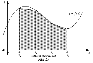
"Graphically, this represents the area of a trapezoid used to approximate the area under the function $f(x)$\n",
"\n",
"
](#top)\n",
"\n",
"Consider the element stiffness\n",
"\n",
"$$\n",
"K_{ij}^{(e)} = \\int_{x_1^{(e)}}^{x_2^{(e)}} a^{(e)} \\phi'_i \\phi'_j dx\n",
"$$\n",
"\n",
"In the event that $a_e$ is a complicated function of $x$, the exact evaluation of the stiffness may not be possible. In such cases, numerical integration is necessary. Likewise, with other integrals encountered in the FEM.\n",
"\n",
"Numerical evaluation of integrals is called numerical quadrature and typically involves approximating the integrand by a polynomial of sufficient degree.\n",
"\n",
"For example, consider the integral\n",
"\n",
"$$\n",
"J[f] = \\int_{x_A}^{x_B} f(x) dx\n",
"$$\n",
"\n",
"We approximate $f(x)$ by\n",
"\n",
"$$\n",
"f(x) \\approx \\sum_i^n f(x_i) \\phi_i(x)\n",
"$$\n",
"\n",
"where the $x_i$ are the $i^{\\rm th}$ point of the interval $[x_A, x_B]$ and $\\phi_i(x_i)$ are polynomials of degree $n-1$. Substitution of the approximate solution for $f$ in to the integral equation gives\n",
"\n",
"$$\n",
"\\begin{align}\n",
"J[f] &= \\int_{x_A}^{x_B} f(x) dx \\\\\n",
" &\\approx \\sum_{i=1}^n f(x_i) \\int_{x_A}^{x_B} \\phi_i(x) dx \\\\\n",
"& = f(x_1) \\int_{x_A}^{x_B} \\phi_1(x) dx + \\ldots + f(x_N) \\int_{x_A}^{x_B} \\phi_n(x) dx\n",
"\\end{align}\n",
"$$\n",
"\n",
"Suppose we choose Lagrange linear interpolation polynomials for the approximation of $f$ with $n=2$. Then\n",
"\n",
"$$\n",
"J[f] \\approx f(x_A) \\int_{x_A}^{x_B} \\frac{x_B - x}{h} dx + f(x_B) \\int_{x_A}^{x_B} \\frac{x - x_A}{h} dx = \\frac{1}{2}h\\left(f(x_A) + f(x_B)\\right)\n",
"$$\n",
"\n",
"Graphically, this represents the area of a trapezoid used to approximate the area under the function $f(x)$\n",
"\n",
" \n",
"\n",
"This is known as the trapzoidal rule. If we use quadratic Lagrange interpolation of $f(x)$ we obtain\n",
"\n",
"$$\n",
"J[f] \\approx \\frac{1}{6}h \\left(f(x_A) + 4 f(x_A + \\frac{1}{2}h) + f(x_B)\\right)\n",
"$$\n",
"\n",
"The previous examples demonstrate the basic idea behind numerical quadrature. In the trapezoidal type rules, we choose the $x_i$ and the weights shake out naturally. It can be shown that this form of numerical integration is exact for polynomials of up to degree $n-1$. The trapezoidal rules also demonstrate a more general form of numerical quadrature:\n",
"\n",
"$$\n",
"\\begin{align}\n",
"J[f] &= \\int_{x_A}^{x_B} f(x) w(x) dx \\\\\n",
"J_n[f] &= \\int_{x_A}^{x_B}w(x) \\sum_{i=1}^n f(x_i) L_i(x) \n",
"= \\sum_{i=1}^n w_i f(x_i)\n",
"\\end{align}\n",
"$$\n",
"\n",
"with\n",
"\n",
"$$\n",
"w_i = \\int_{x_A}^{x_B}L_i(x)w(x) dx, \\quad \n",
"L_i^n(x)=\\prod_{\\stackrel{j=1}{j \\neq i}}^n \\frac{x-x_j}{x_j-x_i}\n",
"$$\n",
"\n",
"where the $x_i$ are called quadrature points, $w_i$ are quadrature weights, and $L_i(x)$ are $n^{\\text{th}}$ order Lagrange polynomials. The goal of numerical quadrature is to choose the $x_i$ and the $w_i$ such that $J_n$ is exact for polynomials up to degree $2n-1$."
]
},
{
"cell_type": "markdown",
"metadata": {},
"source": [
"# Gauss-Legendre Quadrature[](#top)\n",
"\n",
"So, how do we choose the $x_i$ and $w_i$? That question is the subject of numerical analysis, and the exact details are beyond the scope of this class. Here, we seek to determine the quadrature points and weights for small $n$ and appeal to reason and mathematical proofs to furnish the results for all $n$. To that end, we consider only the special case that $w(x)=1$, $a=-1$, $b=1$, and $f(x) \\in P_n$, where $P_n$ is the space of polynomials of degree $n$. This quadrature rule is known as Gauss-Legendre quadrature. Other quadrature rules are distinguished by their choice of $w$, $a$, and $b$.\n",
"\n",
"So, how do we go about finding the $x_i$ and $w_i$? Suppose we want to determine the $w_i$ and $x_i$ for $n=2$:\n",
"\n",
"$$\n",
"\\begin{align}\n",
"J_2[f] &= \\sum_{i=1}^2 f(x_i) \\int_{-1}^{1} L_i(x) = w_1 f(x_1) + w_2 f(x_2)\n",
"\\end{align}\n",
"$$\n",
"\n",
"Evidently, to solve for the unkown $w_i$ and $x_i$, we need 4 equations. Let us form them by considering the first four polynomials $f=1, x, x^2, x^3$:\n",
"\n",
"$$\n",
"\\begin{align}\n",
"w_1 \\cdot 1 + w_2 \\cdot 1 = \\int_{-1}^1 dx = 2 &\\qquad\n",
"w_1 \\cdot x_1 + w_2 \\cdot x_2 = \\int_{-1}^1 x dx = 0 \\\\\n",
"w_1 \\cdot x_1^2 + w_2 \\cdot x_2^2 = \\int_{-1}^1 x^2 dx = \\frac{2}{3} &\\qquad\n",
"w_1 \\cdot x_1^3 + w_2 \\cdot x_2^3 = \\int_{-1}^1 x^3 dx = 0\n",
"\\end{align}\n",
"$$\n",
"\n",
"After some algebra and using the methods of undetermined coefficients to solve the nonlinear system of equations, we find that\n",
"\n",
"$$\n",
"w_1 = w_2 = 1, \\qquad x_1 = -x_2 = -\\frac{\\sqrt{3}}{3}\n",
"$$\n",
"\n",
"and\n",
"\n",
"$$\n",
"J_2[f] = f\\left(-\\frac{\\sqrt{3}}{3}\\right) + f\\left(\\frac{\\sqrt{3}}{3}\\right)\n",
"$$\n",
"\n",
"This is called a 2 point Gauss-Legendre quadrature rule. **The Gauss-Legendre quadrature rule gives exact results if $f(x)$ is a polynomial of degree $2n-1$.**\n",
"\n",
"How can we find the $w_i$ and $x_i$ for higher order Gauss-Legendre quadrature? We can go through the same process as with $n=2$, but it is slow and tedious. Instead, using properties of orthogonal polynomials, the $x_i$ and $w_i$ can be derived for many $w_x$ and domains of integration $[a, b]$. For Gauss-Legendre quadrature, it turns out that the $x_i$ are the roots of the $n^{\\text{th}}$ order Legendre polynomial. The $w_i$ can then be found from knowledge of the $x_i$ and properties of the Legendre polynomials. The details are beyond the scope of this class, but tabulated values of the $x_i$ and $w_i$ can be found in Table 4.1 of the text."
]
},
{
"cell_type": "markdown",
"metadata": {},
"source": [
"# Natural Coordinates[](#top)\n",
"\n",
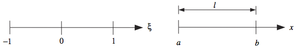
"To make use of the results from the previous section, the domain of integration for an integral of interest must be $[-1,1]$. For integration of element functions, this implies that we must perform a change of coordinates from the element domain $[x_1^{(e)},x_2^{(e)}]$ to $[-1,1]$. The transformed domain $[-1, 1]$ is referred to as the **natural coordinates**. The actual element domain will be referred to as the **physical coordinates**. To distinguish natural coordinates from the physical coordinates, the natural coordinates will be labeled $\\xi$.\n",
"\n",
"Mathematically, we seek a transformation such that \n",
"\n",
"$$\n",
"\\xi = \\begin{cases}\n",
"-1 & \\text{for } x = x_1^{(e)} \\\\\n",
"1 & \\text{for } x = x_2^{(e)} \\\\\n",
"\\end{cases}\n",
"$$\n",
"\n",
"Then the transformation between $x$ and $\\xi$ can be represented by\n",
"\n",
"$$\n",
"x = a + b\\xi\n",
"$$\n",
"\n",
"which is known as a \"stretch\" transformation. We determine the constants $a$ and $b$ be requiring that\n",
"\n",
"$$\n",
"\\begin{align}\n",
"x_1^{(e)} &= a + b(-1) \\\\\n",
"x_2^{(e)} &= a + b(1)\n",
"\\end{align}\n",
"$$\n",
"\n",
"Solving for $a$ and $b$ we get\n",
"\n",
"$$\n",
"a = b = \\frac{1}{2} h^{(e)}\n",
"$$\n",
"\n",
"Then, the transformation becomes\n",
"\n",
"$$\n",
"x = x_1^{(e)} + \\frac{1}{2}h^{(e)} \\left( 1 + \\xi \\right)\n",
"$$\n",
"\n",
"where $x_1^{(e)}$ denotes the left end node of the element and $h^{(e)}$ is the element length. \n",
"\n",
"The value of the natural coordinate always lies in $[-1,1]$ with origin at the element center, as shown:\n",
"\n",
"
\n",
"\n",
"This is known as the trapzoidal rule. If we use quadratic Lagrange interpolation of $f(x)$ we obtain\n",
"\n",
"$$\n",
"J[f] \\approx \\frac{1}{6}h \\left(f(x_A) + 4 f(x_A + \\frac{1}{2}h) + f(x_B)\\right)\n",
"$$\n",
"\n",
"The previous examples demonstrate the basic idea behind numerical quadrature. In the trapezoidal type rules, we choose the $x_i$ and the weights shake out naturally. It can be shown that this form of numerical integration is exact for polynomials of up to degree $n-1$. The trapezoidal rules also demonstrate a more general form of numerical quadrature:\n",
"\n",
"$$\n",
"\\begin{align}\n",
"J[f] &= \\int_{x_A}^{x_B} f(x) w(x) dx \\\\\n",
"J_n[f] &= \\int_{x_A}^{x_B}w(x) \\sum_{i=1}^n f(x_i) L_i(x) \n",
"= \\sum_{i=1}^n w_i f(x_i)\n",
"\\end{align}\n",
"$$\n",
"\n",
"with\n",
"\n",
"$$\n",
"w_i = \\int_{x_A}^{x_B}L_i(x)w(x) dx, \\quad \n",
"L_i^n(x)=\\prod_{\\stackrel{j=1}{j \\neq i}}^n \\frac{x-x_j}{x_j-x_i}\n",
"$$\n",
"\n",
"where the $x_i$ are called quadrature points, $w_i$ are quadrature weights, and $L_i(x)$ are $n^{\\text{th}}$ order Lagrange polynomials. The goal of numerical quadrature is to choose the $x_i$ and the $w_i$ such that $J_n$ is exact for polynomials up to degree $2n-1$."
]
},
{
"cell_type": "markdown",
"metadata": {},
"source": [
"# Gauss-Legendre Quadrature[](#top)\n",
"\n",
"So, how do we choose the $x_i$ and $w_i$? That question is the subject of numerical analysis, and the exact details are beyond the scope of this class. Here, we seek to determine the quadrature points and weights for small $n$ and appeal to reason and mathematical proofs to furnish the results for all $n$. To that end, we consider only the special case that $w(x)=1$, $a=-1$, $b=1$, and $f(x) \\in P_n$, where $P_n$ is the space of polynomials of degree $n$. This quadrature rule is known as Gauss-Legendre quadrature. Other quadrature rules are distinguished by their choice of $w$, $a$, and $b$.\n",
"\n",
"So, how do we go about finding the $x_i$ and $w_i$? Suppose we want to determine the $w_i$ and $x_i$ for $n=2$:\n",
"\n",
"$$\n",
"\\begin{align}\n",
"J_2[f] &= \\sum_{i=1}^2 f(x_i) \\int_{-1}^{1} L_i(x) = w_1 f(x_1) + w_2 f(x_2)\n",
"\\end{align}\n",
"$$\n",
"\n",
"Evidently, to solve for the unkown $w_i$ and $x_i$, we need 4 equations. Let us form them by considering the first four polynomials $f=1, x, x^2, x^3$:\n",
"\n",
"$$\n",
"\\begin{align}\n",
"w_1 \\cdot 1 + w_2 \\cdot 1 = \\int_{-1}^1 dx = 2 &\\qquad\n",
"w_1 \\cdot x_1 + w_2 \\cdot x_2 = \\int_{-1}^1 x dx = 0 \\\\\n",
"w_1 \\cdot x_1^2 + w_2 \\cdot x_2^2 = \\int_{-1}^1 x^2 dx = \\frac{2}{3} &\\qquad\n",
"w_1 \\cdot x_1^3 + w_2 \\cdot x_2^3 = \\int_{-1}^1 x^3 dx = 0\n",
"\\end{align}\n",
"$$\n",
"\n",
"After some algebra and using the methods of undetermined coefficients to solve the nonlinear system of equations, we find that\n",
"\n",
"$$\n",
"w_1 = w_2 = 1, \\qquad x_1 = -x_2 = -\\frac{\\sqrt{3}}{3}\n",
"$$\n",
"\n",
"and\n",
"\n",
"$$\n",
"J_2[f] = f\\left(-\\frac{\\sqrt{3}}{3}\\right) + f\\left(\\frac{\\sqrt{3}}{3}\\right)\n",
"$$\n",
"\n",
"This is called a 2 point Gauss-Legendre quadrature rule. **The Gauss-Legendre quadrature rule gives exact results if $f(x)$ is a polynomial of degree $2n-1$.**\n",
"\n",
"How can we find the $w_i$ and $x_i$ for higher order Gauss-Legendre quadrature? We can go through the same process as with $n=2$, but it is slow and tedious. Instead, using properties of orthogonal polynomials, the $x_i$ and $w_i$ can be derived for many $w_x$ and domains of integration $[a, b]$. For Gauss-Legendre quadrature, it turns out that the $x_i$ are the roots of the $n^{\\text{th}}$ order Legendre polynomial. The $w_i$ can then be found from knowledge of the $x_i$ and properties of the Legendre polynomials. The details are beyond the scope of this class, but tabulated values of the $x_i$ and $w_i$ can be found in Table 4.1 of the text."
]
},
{
"cell_type": "markdown",
"metadata": {},
"source": [
"# Natural Coordinates[](#top)\n",
"\n",
"To make use of the results from the previous section, the domain of integration for an integral of interest must be $[-1,1]$. For integration of element functions, this implies that we must perform a change of coordinates from the element domain $[x_1^{(e)},x_2^{(e)}]$ to $[-1,1]$. The transformed domain $[-1, 1]$ is referred to as the **natural coordinates**. The actual element domain will be referred to as the **physical coordinates**. To distinguish natural coordinates from the physical coordinates, the natural coordinates will be labeled $\\xi$.\n",
"\n",
"Mathematically, we seek a transformation such that \n",
"\n",
"$$\n",
"\\xi = \\begin{cases}\n",
"-1 & \\text{for } x = x_1^{(e)} \\\\\n",
"1 & \\text{for } x = x_2^{(e)} \\\\\n",
"\\end{cases}\n",
"$$\n",
"\n",
"Then the transformation between $x$ and $\\xi$ can be represented by\n",
"\n",
"$$\n",
"x = a + b\\xi\n",
"$$\n",
"\n",
"which is known as a \"stretch\" transformation. We determine the constants $a$ and $b$ be requiring that\n",
"\n",
"$$\n",
"\\begin{align}\n",
"x_1^{(e)} &= a + b(-1) \\\\\n",
"x_2^{(e)} &= a + b(1)\n",
"\\end{align}\n",
"$$\n",
"\n",
"Solving for $a$ and $b$ we get\n",
"\n",
"$$\n",
"a = b = \\frac{1}{2} h^{(e)}\n",
"$$\n",
"\n",
"Then, the transformation becomes\n",
"\n",
"$$\n",
"x = x_1^{(e)} + \\frac{1}{2}h^{(e)} \\left( 1 + \\xi \\right)\n",
"$$\n",
"\n",
"where $x_1^{(e)}$ denotes the left end node of the element and $h^{(e)}$ is the element length. \n",
"\n",
"The value of the natural coordinate always lies in $[-1,1]$ with origin at the element center, as shown:\n",
"\n",
" "
]
},
{
"cell_type": "markdown",
"metadata": {},
"source": [
"## Approximation of Geometry\n",
"\n",
"Recall that the element stiffness and force arrays (for second order boundary value problems) are given by\n",
"\n",
"$$\n",
"k_{ij} = \\int_{x_A}^{x_B} a\\phi'_i\\phi'_j + c\\phi_i\\phi_j dx\n",
"$$\n",
"$$\n",
"f_i = \\int_{x_A}^{x_B} q\\phi_i + P\\delta(x - x_i) dx\n",
"$$\n",
"\n",
"These element matrices involve derivatives of the interpolation functions with respect to the physical coordinates $x$. Thus, we need to find a transformation of the form\n",
"\n",
"$$\n",
"x = \\chi(\\xi)\n",
"$$\n",
"\n",
"so that the integrals can be cast in terms of $\\xi$ on $[-1, 1]$. The transformation $\\chi$ is assumed to be 1 to 1. An example of one such transformation is\n",
"\n",
"$$\n",
"\\chi(\\xi) = x_1^{(e)} + \\frac{1}{2}h^{(e)}\\left(1+\\xi\\right)\n",
"$$\n",
"\n",
"which is the same as our original transformation. In this transformation $\\chi(\\xi)$ is a linear function of $\\xi$. It will map a straight line to a straight line. If $\\chi$ were non-linear, it would map a straight line to a curved line.\n",
"\n",
"It is natural to think of approximating the geometry in the same way as we approximated a dependent variable. In other words, the transformation $x=\\chi(\\xi)$ can be written as\n",
"\n",
"$$\n",
"x = \\chi(\\xi) = \\sum_{i=1}^m x_i^{(e)} \\phi_i^{(e)}(\\xi)\n",
"$$\n",
"\n",
"where $x_i^{(e)}$ is the physical coordinate of the $i^{\\rm th}$ node of element $(e)$. $\\phi_i^{(e)}(\\xi)$ are interpolating polynomials of degree $m-1$. This equation represents the shape of the element and the $\\phi_i^{(e)}(\\xi)$ are called the **shape functions**, aften denoted as $\\{N(\\xi)\\}$.\n",
"\n",
"Physically, this mapping maps a geometric shape from $\\xi$ to $x$. In other words, for any given value of $\\xi$ we can determine the corresponding value of $x$. When the element is a straight line, the preceding transformation is the same as that for the linear case.\n",
"\n",
"
"
]
},
{
"cell_type": "markdown",
"metadata": {},
"source": [
"## Approximation of Geometry\n",
"\n",
"Recall that the element stiffness and force arrays (for second order boundary value problems) are given by\n",
"\n",
"$$\n",
"k_{ij} = \\int_{x_A}^{x_B} a\\phi'_i\\phi'_j + c\\phi_i\\phi_j dx\n",
"$$\n",
"$$\n",
"f_i = \\int_{x_A}^{x_B} q\\phi_i + P\\delta(x - x_i) dx\n",
"$$\n",
"\n",
"These element matrices involve derivatives of the interpolation functions with respect to the physical coordinates $x$. Thus, we need to find a transformation of the form\n",
"\n",
"$$\n",
"x = \\chi(\\xi)\n",
"$$\n",
"\n",
"so that the integrals can be cast in terms of $\\xi$ on $[-1, 1]$. The transformation $\\chi$ is assumed to be 1 to 1. An example of one such transformation is\n",
"\n",
"$$\n",
"\\chi(\\xi) = x_1^{(e)} + \\frac{1}{2}h^{(e)}\\left(1+\\xi\\right)\n",
"$$\n",
"\n",
"which is the same as our original transformation. In this transformation $\\chi(\\xi)$ is a linear function of $\\xi$. It will map a straight line to a straight line. If $\\chi$ were non-linear, it would map a straight line to a curved line.\n",
"\n",
"It is natural to think of approximating the geometry in the same way as we approximated a dependent variable. In other words, the transformation $x=\\chi(\\xi)$ can be written as\n",
"\n",
"$$\n",
"x = \\chi(\\xi) = \\sum_{i=1}^m x_i^{(e)} \\phi_i^{(e)}(\\xi)\n",
"$$\n",
"\n",
"where $x_i^{(e)}$ is the physical coordinate of the $i^{\\rm th}$ node of element $(e)$. $\\phi_i^{(e)}(\\xi)$ are interpolating polynomials of degree $m-1$. This equation represents the shape of the element and the $\\phi_i^{(e)}(\\xi)$ are called the **shape functions**, aften denoted as $\\{N(\\xi)\\}$.\n",
"\n",
"Physically, this mapping maps a geometric shape from $\\xi$ to $x$. In other words, for any given value of $\\xi$ we can determine the corresponding value of $x$. When the element is a straight line, the preceding transformation is the same as that for the linear case.\n",
"\n",
"\n",
"\n",
"The transformation is not used to change the actual geometry of the element - the transformation is used to write\n",
"\n",
"$$\n",
"\\int_{x_1^{(e)}}^{x_2^{(e)}}f(x)dx = \\int_{-1}^{1}f(\\xi)d\\xi\n",
"$$\n",
"\n",
"so that Gauss quadrature can be used to approximate the integral.\n",
"\n",
"
\n",
"\n",
"To complete the transformation, we need $dx$ in terms of $d\\xi$. $dx$ in the global coordinates is related to $d\\xi$ by\n",
"\n",
"$$\n",
"dx = \\frac{\\partial x}{\\partial \\xi} d\\xi = J^{(e)} d\\xi\n",
"$$\n",
"\n",
"where $J^{(e)}$ is called the \"Jacobian\" of the transformation. Using our transformation, we have\n",
"\n",
"$$\n",
"J^{(e)} = \\frac{\\partial x}{\\partial \\xi} =\n",
"\\frac{\\partial }{\\partial \\xi} \\sum_{i=1}^{m} x_i^{(e)}\\frac{\\partial \\phi_i^{(e)}(\\xi)}{\\partial \\xi}\n",
"$$"
]
},
{
"cell_type": "markdown",
"metadata": {},
"source": [
"## \\*Parametric Formulations\n",
"\n",
"Recall that our approximate solution is of the form\n",
"\n",
"$$\n",
"u_N(x) = \\sum_{j=1}^{n} u_j \\phi_j(x)\n",
"$$\n",
"\n",
"In general, the degree of the transformation $m$ does not have to equal the degree of the approximation $n$. In other words, $\\phi_i(x) \\neq \\phi_i(\\xi)$.\n",
"\n",
"Two elements can be used in the finite element analysis: one for the approximation of the geometry and the other for the interpolation of $u$. Finite element formulations are classified as\n",
"\n",
"- Subparametric: m < n\n",
"- Isoparametric: m = n\n",
"- Superparametric: m > n\n",
"\n",
"Examples:\n",
"\n",
"- Subparametric: In the Euler-Bernouli beam element the transverse deflection is approximated by the cubic Hermite polynomials and straight beams are approximated by linear polynomials.\n",
"- Isoparametric: The same element is used to approximate the geometry and dependent variable.\n",
"- Superparametric: The geometry is approximated by higher order polynomial than the dependent variable. Rarely used in practice."
]
},
{
"cell_type": "markdown",
"metadata": {},
"source": [
"# Examples[](#top)\n",
"\n",
"## Example 1: Element Stiffness\n",
"\n",
"We now piece together what we have done so far. Consider the FE stiffness matrix in global coordinates\n",
"\n",
"$$\n",
"k_{ij}^{(e)} = \\int_{x_A}^{x_B} a_e \\frac{d\\phi_i^{(e)}}{dx} \\frac{d\\phi_j^{(e)}}{dx} dx\n",
"$$\n",
"\n",
"To transform the the integral from $x$ to $\\xi$, we note that\n",
"\n",
"$$\n",
"a(x) = a(\\chi(\\xi)), \\quad dx = Jd\\xi\n",
"$$\n",
"\n",
"$$\n",
"\\frac{d\\phi}{dx} = \\frac{d\\phi}{d\\xi}\\frac{d\\xi}{dx} = \\frac{1}{J}\\frac{d\\phi}{d\\xi}\n",
"$$\n",
"\n",
"Therefore, the stiffness can be written as\n",
"\n",
"$$\\begin{align}\n",
"k_{ij}^{(e)} &= \\int_{-1}^{1} a^{(e)}(\\chi(\\xi)) \n",
" \\frac{1}{J^{(e)}}\\frac{d\\phi_i^{(e)}}{d\\xi}\\frac{1}{J^{(e)}}\\frac{d\\phi_j^{(e)}}{d\\xi}\n",
" J d\\xi \\\\\n",
" &= \\int_{-1}^{1} \\frac{a^{(e)}(\\chi(\\xi))}{J^{(e)}} \\frac{d\\phi_i^{(e)}}{d\\xi}\\frac{d\\phi_j^{(e)}}{d\\xi}d\\xi \\\\\n",
" &= \\sum_{I=1}^n Q_{ij}^{(e)}\\left(\\xi_I\\right)w_I\n",
"\\end{align}\n",
"$$\n",
"\n",
"where\n",
"\n",
"$$\n",
"Q_{ij}^{(e)} = \\frac{a^{(e)}}{J^{(e)}} \\frac{d\\phi_i^{(e)}}{d\\xi}\\frac{d\\phi_j^{(e)}}{d\\xi}\n",
"$$\n",
"\n",
"For linear interpolation elements and an isoparametric mapping, the shape functions are\n",
"\n",
"$$\n",
"\\{\\phi(\\xi)\\}^{(e)}\n",
"= \\frac{1}{2}\n",
"\\begin{Bmatrix}\n",
"1 - \\xi \\\\\n",
"1 + \\xi\n",
"\\end{Bmatrix}\n",
"$$\n",
"\n",
"and\n",
"\n",
"$$\n",
"J = \\sum_{i=1}^m x_i^{(e)} \\frac{d\\phi_i^{(e)}}{d\\xi} = \\frac{1}{2}\\left(x_1(-1) + x_2(1)\\right) = \\frac{1}{2}h^{(e)}\n",
"$$\n",
"\n",
"For elementwise constant values of $a$ and $h$\n",
"\n",
"$$\\begin{align}\n",
"k_{ij}^{(e)} &= Q_{ij}^{(e)}(\\xi_1) w_1 + Q_{ij}^{(e)}(\\xi_2) w_2 \\\\\n",
" &= \\frac{2a^{(e)}}{h^{(e)}}\\left(2\\frac{d\\phi_i^{(e)}}{d\\xi}\\frac{d\\phi_j^{(e)}}{d\\xi}\\right)\n",
"\\end{align}\n",
"$$\n",
"\n",
"from which\n",
"\n",
"$$ k_{11}^{(e)} = \\frac{2a^{(e)}}{h^{(e)}} \\left(2(-.5)(-.5)\\right) = \\frac{a}{h}^{(e)} $$\n",
"$$ k_{12}^{(e)} = \\frac{2a^{(e)}}{h^{(e)}} \\left(2(-.5)(.5)\\right) = -\\frac{a}{h}^{(e)} $$\n",
"$$ k_{21}^{(e)} = \\frac{2a^{(e)}}{h^{(e)}} \\left(2(.5)(-.5)\\right) = -\\frac{a}{h}^{(e)} $$\n",
"$$ k_{22}^{(e)} = \\frac{2a^{(e)}}{h^{(e)}} \\left(2(.5)(.5)\\right) = \\frac{a}{h}^{(e)} $$\n",
"\n",
"and\n",
"\n",
"$$\n",
"[k]^{(e)} = \\frac{a^{(e)}}{h^{(e)}} \\begin{bmatrix} 1 & -1 \\\\ -1 & 1 \\end{bmatrix}\n",
"$$\n",
"\n",
"As noted before, the Jacobian matrix will be the same - $J^{(e)} = h^{(e)} / 2$ - when the element is straight, even when the coordinate transformation is not linear. However, when the element is curved, the Jacobian is a function of $\\xi$ for transformations other than linear."
]
},
{
"cell_type": "markdown",
"metadata": {},
"source": [
"## Example 2: Reduced Integration\n",
"\n",
"It is often beneficial to reduce the number of integration points that are evaluated. In the case of the element stiffness with constant properties, single point Gauss-Legendre quadrature can be used to find $k_{ij}^{(e)}$ exactly:\n",
"\n",
"$$\n",
"\\begin{align}\n",
"k_{ij} &= Q_{ij}^{(e)}(\\xi_1)w_1 \\\\\n",
"&= \\frac{2a^{(e)}}{h^{(e)}}\\left(\\frac{d\\phi_i^{(e)}}{d\\xi}\\frac{d\\phi_j^{(e)}}{d\\xi}\\right) 2 \\\\\n",
"& = \\frac{a^{(e)}}{h^{(e)}} \\begin{bmatrix} 1 & -1 \\\\ -1 & 1 \\end{bmatrix}\n",
"\\end{align}\n",
"$$\n",
"\n",
"where we used the fact that $w_1=2$ for single point integration.\n",
"\n",
"It turns out that in higher dimensions, using reduced integration can have a dramatic influence on the finite element solution - both good and bad!"
]
}
],
"metadata": {
"kernelspec": {
"display_name": "Python 2",
"language": "python",
"name": "python2"
},
"language_info": {
"codemirror_mode": {
"name": "ipython",
"version": 2
},
"file_extension": ".py",
"mimetype": "text/x-python",
"name": "python",
"nbconvert_exporter": "python",
"pygments_lexer": "ipython2",
"version": "2.7.9"
}
},
"nbformat": 4,
"nbformat_minor": 0
}