{
"cells": [
{
"cell_type": "code",
"execution_count": 2,
"metadata": {
"collapsed": false
},
"outputs": [
{
"data": {
"text/html": [
"\n"
],
"text/plain": [
""
]
},
"execution_count": 2,
"metadata": {},
"output_type": "execute_result"
}
],
"source": [
"import theme\n",
"theme.load_style()"
]
},
{
"cell_type": "markdown",
"metadata": {},
"source": [
"# Higher Order Shape Functions\n",
"\n",
" \n",
"\n",
"This lecture by Tim Fuller is licensed under the\n",
"Creative Commons Attribution 4.0 International License. All code examples are also licensed under the [MIT license](http://opensource.org/licenses/MIT)."
]
},
{
"cell_type": "markdown",
"metadata": {},
"source": [
"\n",
"\n",
"# Topics\n",
"\n",
"- [Introduction](#intro)\n",
"- [Quadratic Shape Functions](#quad-sf)\n",
" - [Direct Construction of Quadratic Shape Functions](#dir-quad-sf)\n",
"- [Direct Construction of Shape Functions in Natural Coordinates](#dir-nat-sf)\n",
" - [Linear Shape Functions in Natural Coordinates](#nat-lin-sf)\n",
" - [Quadratic Shape Functions in Natural Coordinates](#nat-quad-sf)\n",
" - [Higher Order Shape Functions in Natural Coordinates](#nat-higher-sf)\n",
"- [Example](#example)"
]
},
{
"cell_type": "markdown",
"metadata": {},
"source": [
"# Introduction[
\n",
"\n",
"This lecture by Tim Fuller is licensed under the\n",
"Creative Commons Attribution 4.0 International License. All code examples are also licensed under the [MIT license](http://opensource.org/licenses/MIT)."
]
},
{
"cell_type": "markdown",
"metadata": {},
"source": [
"\n",
"\n",
"# Topics\n",
"\n",
"- [Introduction](#intro)\n",
"- [Quadratic Shape Functions](#quad-sf)\n",
" - [Direct Construction of Quadratic Shape Functions](#dir-quad-sf)\n",
"- [Direct Construction of Shape Functions in Natural Coordinates](#dir-nat-sf)\n",
" - [Linear Shape Functions in Natural Coordinates](#nat-lin-sf)\n",
" - [Quadratic Shape Functions in Natural Coordinates](#nat-quad-sf)\n",
" - [Higher Order Shape Functions in Natural Coordinates](#nat-higher-sf)\n",
"- [Example](#example)"
]
},
{
"cell_type": "markdown",
"metadata": {},
"source": [
"# Introduction[ ](#top)\n",
"\n",
"In previous lectures, we have approximated the solution to the governing equations with linear shape functions. Higher order approximate solutions, often times, can lead to increased accuracy, especially when extracting derivative values from the solution (i.e. stress and strain)."
]
},
{
"cell_type": "markdown",
"metadata": {},
"source": [
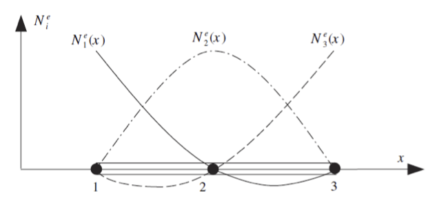
"# Quadratic Shape Functions[](#top)\n",
"\n",
"Approximate the dependent variable $u$ by a quadratic function\n",
"\n",
"$$\n",
"U_N = a + b x + c x ^ 2\n",
"= \\begin{pmatrix} 1 & x & x^2 \\end{pmatrix}\n",
" \\begin{pmatrix} a \\\\ b \\\\ c \\end{pmatrix}\n",
"= \\boldsymbol{p}(x) \\boldsymbol{\\alpha}\n",
"$$\n",
"\n",
"We want to express the approximate solution to $u$ in terms of nodal displacements and not the constant coefficients $a$, $b$, and $c$. Thus, we force the approximate solution $u$ to be equal to nodal displacements $u_1$, $u_2$, and $u_3$ and $x_1$, $x_2$, and $x_3$, respectively, on some finite element.\n",
"\n",
"$$\n",
"\\begin{align}\n",
" u_1 &= a + b x_1 + c x_1^2 \\\\\n",
" u_2 &= a + b x_2 + c x_2^2 \\\\\n",
" u_3 &= a + b x_3 + c x_3^2 \\\\\n",
"\\end{align} \\longrightarrow\n",
"\\begin{pmatrix} u_1 \\\\ u_2 \\\\ u_3 \\end{pmatrix} =\n",
"\\begin{pmatrix} \n",
"1 & x_1 & x_1^2 \\\\ 1 & x_2 & x_2^2 \\\\ 1 & x_3 & x_3^2\n",
"\\end{pmatrix}\n",
"\\begin{pmatrix} a \\\\ b \\\\ c \\end{pmatrix} \n",
"\\longrightarrow \\boldsymbol{d} = \\boldsymbol{M} \\boldsymbol{\\alpha}\n",
"$$\n",
"\n",
"Then,\n",
"\n",
"$$\n",
"U_N = \\boldsymbol{p} \\boldsymbol{M}^{-1} \\boldsymbol{d} = \n",
"\\boldsymbol{N} \\boldsymbol{d} = \\sum_{i=1}^3 N_i(x)u_i\n",
"$$\n",
"\n",
"where the shape functions $N_i$ are\n",
"\n",
"$$\n",
"N_i = \\frac{2}{h_e^2} \n",
"\\begin{pmatrix}\n",
" \\left(x - x_2\\right)\\left(x - x_3\\right) \\\\\n",
" -2\\left(x - x_1\\right)\\left(x - x_3\\right) \\\\\n",
" \\left(x - x_1\\right)\\left(x - x_2\\right) \\\\\n",
"\\end{pmatrix}\n",
"$$\n",
"\n",
"
](#top)\n",
"\n",
"In previous lectures, we have approximated the solution to the governing equations with linear shape functions. Higher order approximate solutions, often times, can lead to increased accuracy, especially when extracting derivative values from the solution (i.e. stress and strain)."
]
},
{
"cell_type": "markdown",
"metadata": {},
"source": [
"# Quadratic Shape Functions[](#top)\n",
"\n",
"Approximate the dependent variable $u$ by a quadratic function\n",
"\n",
"$$\n",
"U_N = a + b x + c x ^ 2\n",
"= \\begin{pmatrix} 1 & x & x^2 \\end{pmatrix}\n",
" \\begin{pmatrix} a \\\\ b \\\\ c \\end{pmatrix}\n",
"= \\boldsymbol{p}(x) \\boldsymbol{\\alpha}\n",
"$$\n",
"\n",
"We want to express the approximate solution to $u$ in terms of nodal displacements and not the constant coefficients $a$, $b$, and $c$. Thus, we force the approximate solution $u$ to be equal to nodal displacements $u_1$, $u_2$, and $u_3$ and $x_1$, $x_2$, and $x_3$, respectively, on some finite element.\n",
"\n",
"$$\n",
"\\begin{align}\n",
" u_1 &= a + b x_1 + c x_1^2 \\\\\n",
" u_2 &= a + b x_2 + c x_2^2 \\\\\n",
" u_3 &= a + b x_3 + c x_3^2 \\\\\n",
"\\end{align} \\longrightarrow\n",
"\\begin{pmatrix} u_1 \\\\ u_2 \\\\ u_3 \\end{pmatrix} =\n",
"\\begin{pmatrix} \n",
"1 & x_1 & x_1^2 \\\\ 1 & x_2 & x_2^2 \\\\ 1 & x_3 & x_3^2\n",
"\\end{pmatrix}\n",
"\\begin{pmatrix} a \\\\ b \\\\ c \\end{pmatrix} \n",
"\\longrightarrow \\boldsymbol{d} = \\boldsymbol{M} \\boldsymbol{\\alpha}\n",
"$$\n",
"\n",
"Then,\n",
"\n",
"$$\n",
"U_N = \\boldsymbol{p} \\boldsymbol{M}^{-1} \\boldsymbol{d} = \n",
"\\boldsymbol{N} \\boldsymbol{d} = \\sum_{i=1}^3 N_i(x)u_i\n",
"$$\n",
"\n",
"where the shape functions $N_i$ are\n",
"\n",
"$$\n",
"N_i = \\frac{2}{h_e^2} \n",
"\\begin{pmatrix}\n",
" \\left(x - x_2\\right)\\left(x - x_3\\right) \\\\\n",
" -2\\left(x - x_1\\right)\\left(x - x_3\\right) \\\\\n",
" \\left(x - x_1\\right)\\left(x - x_2\\right) \\\\\n",
"\\end{pmatrix}\n",
"$$\n",
"\n",
" \n",
"\n",
"## Direct Construction of Quadratic Shape Functions\n",
"\n",
"The method previously described is applicable to shape functions of any order, but, as you can imagine, the process becomes extremely involved and difficult for elements of order higher than 3 or so. Fortunately, using the properties of shape functions that\n",
"\n",
"- the sum of all shape functions sums to 1 at all points (**partition of unity**)\n",
"- the i$^\\mathrm{th}$ shape function has the Kronecker delta property and is the only non‐zero function in the series at node i, where it has a value of 1.\n",
"\n",
"any order shape function can be constructed directly. For example, from the properties of shape functions we construct the quadratic shape function $N_1$ as\n",
"\n",
"$$\n",
"\\begin{align}\n",
" \\text{General form of a quadratic product of monomials} &\\quad N_1 = \\frac{(x-a)(x-b)}{c} \\\\ \n",
" \\text{Kronecker delta property} &\\quad N_1 = \\frac{(x-x_2)(x-x_3)}{c} \\\\\n",
" N_x(x_1) = 1 &\\quad N_1 = \\frac{(x-x_2)(x-x_3)}{(x_1-x_2)(x_1-x_3)} \\\\\n",
"\\end{align}\n",
"$$"
]
},
{
"cell_type": "markdown",
"metadata": {},
"source": [
"# Direct Construction of Shape Functions in Natural Coordinates[](#top)\n",
"\n",
"As discussed in [Lesson 12](Lesson12_NumericalIntegration.ipynb), for integration purposes, it is convenient to express element shape functions in the natural coordinates. It turns out that since the element shape functions are interpolating polynomials, they can be formulated in the natural coordinates by normalizing the appropriate Lagrange interpolation functions in terms of $\\xi$. For an element of $n$ nodes, the $n^{\\text{th}}$ Lagrange interpolating functions are formed such that\n",
"\n",
"\n",
"$$\n",
"L_i^n = c_i\\left(\\xi-\\xi_1\\right)\\left(\\xi-\\xi_2\\right)\n",
"\\cdots\n",
"\\left(\\xi-\\xi_{i-1}\\right)\\left(\\xi-\\xi_{i+1}\\right)\n",
"\\cdots\n",
"\\left(\\xi-\\xi_n\\right)\n",
"$$\n",
"\n",
"The $c_i$ are found by noting that \n",
"\n",
"$$\n",
"L_i^n(\\xi_j) = \\begin{cases}\n",
"1 & i = j \\\\\n",
"0 & \\text{otherwise}\n",
"\\end{cases}\n",
"$$\n",
"\n",
"Thus the $c_i$ are given by\n",
"\n",
"$$\n",
"c_i = \\frac{1}{\n",
"\\left(\\xi_i-\\xi_1\\right)\\left(\\xi_i-\\xi_2\\right)\n",
"\\cdots\n",
"\\left(\\xi_i-\\xi_{i-1}\\right)\\left(\\xi_i-\\xi_{i+1}\\right)\n",
"\\cdots\n",
"\\left(\\xi_i-\\xi_n\\right)}\n",
"$$\n",
"\n",
"Then $L_i^n$ is\n",
"\n",
"$$\n",
"L_i^n = \\frac{\\left(\\xi-\\xi_1\\right)\\left(\\xi-\\xi_2\\right)\n",
"\\cdots\n",
"\\left(\\xi-\\xi_{i-1}\\right)\\left(\\xi-\\xi_{i+1}\\right)\n",
"\\cdots\n",
"\\left(\\xi-\\xi_n\\right)}{\n",
"\\left(\\xi_i-\\xi_1\\right)\\left(\\xi_i-\\xi_2\\right)\n",
"\\cdots\n",
"\\left(\\xi_i-\\xi_{i-1}\\right)\\left(\\xi_i-\\xi_{i+1}\\right)\n",
"\\cdots\n",
"\\left(\\xi_i-\\xi_n\\right)}\n",
"$$\n",
"\n",
"Formed in this way, the $L_i^n$ are the element shape functions $\\phi_i$, expressed in the natural coordinates $\\xi$.\n",
"\n",
"Interpolation functions of this form are said to belong to the Lagrange family of interpolation polynomials. The finite element models based on Lagrange interpolation polynomials are said to belong to the Lagrange family of finite elements. All of the elements encountered in this course, thus far, have been Lagrange finite elements."
]
},
{
"cell_type": "markdown",
"metadata": {},
"source": [
"## Linear Lagrange Shape Functions\n",
"\n",
"For a linear linear two node element, the shape functions are found from the linear Lagrange interpolating functions:\n",
"\n",
"$$\n",
"\\phi_1(\\xi) = L_1^1(\\xi) = \\frac{\\xi - \\xi_2}{\\xi_1 - \\xi_2} = \\frac{\\xi - 1}{(-1) - 1} = -\\frac{\\xi - 1}{2}\n",
"$$\n",
"$$\n",
"\\phi_2(\\xi) = L_2^1(\\xi) = \\frac{\\xi - \\xi_1}{\\xi_2 - \\xi_1} = \\frac{\\xi - (-1)}{1 - (-1)} = \\frac{\\xi +1}{2}\n",
"$$\n",
"\n",
"Or\n",
"\n",
"$$\n",
"\\{\\phi\\} \n",
"= \\frac{1}{2}\n",
"\\begin{Bmatrix}\n",
"1 - \\xi \\\\\n",
"1 + \\xi\n",
"\\end{Bmatrix}\n",
"$$"
]
},
{
"cell_type": "markdown",
"metadata": {},
"source": [
"## Quadratic Lagrange Shape Functions\n",
"\n",
"For a linear linear two node element, the shape functions are found from the quadratic Lagrange interpolating functions with $\\xi_1=-1$, $\\xi_2=1$, $\\xi_3=0$:\n",
"\n",
"$$\n",
"\\begin{align}\n",
"\\phi_1(\\xi) = L_1^2(\\xi) &= \\frac{\\left(\\xi-\\xi_2\\right)\\left(\\xi-\\xi_3\\right)}\n",
" {\\left(\\xi_1-\\xi_2\\right)\\left(\\xi_1-\\xi_3\\right)}\n",
" = \\frac{\\xi\\left(\\xi-1\\right)}{2} \\\\\n",
"\\phi_2(\\xi) = L_2^2(\\xi) &= \\frac{\\left(\\xi-\\xi_1\\right)\\left(\\xi-\\xi_3\\right)}\n",
" {\\left(\\xi_2-\\xi_1\\right)\\left(\\xi_2-\\xi_3\\right)} \n",
" = \\frac{\\xi\\left(\\xi+1\\right)}{2} \\\\\n",
"\\phi_3(\\xi) = L_3^2(\\xi) &= \\frac{\\left(\\xi-\\xi_1\\right)\\left(\\xi-\\xi_2\\right)}\n",
" {\\left(\\xi_3-\\xi_1\\right)\\left(\\xi_3-\\xi_2\\right)} \n",
" = -\\left(\\xi+1\\right)\\left(\\xi-1\\right)\n",
"\\end{align}\n",
"$$\n",
"\n",
"$$\n",
"\\phi_i = \\frac{1}{2}\n",
"\\begin{Bmatrix}\n",
"-\\xi(1 - \\xi) \\\\ \\xi(1+\\xi) \\\\ 2(1 + \\xi)(1 - \\xi)\\\\\n",
"\\end{Bmatrix}\n",
"$$\n",
"\n",
"### Isoparametric Mapping\n",
"\n",
"Based on our choice of the $\\xi_i$, the isoparametric mapping for the quadratic map looks like\n",
"\n",
"
\n",
"\n",
"## Direct Construction of Quadratic Shape Functions\n",
"\n",
"The method previously described is applicable to shape functions of any order, but, as you can imagine, the process becomes extremely involved and difficult for elements of order higher than 3 or so. Fortunately, using the properties of shape functions that\n",
"\n",
"- the sum of all shape functions sums to 1 at all points (**partition of unity**)\n",
"- the i$^\\mathrm{th}$ shape function has the Kronecker delta property and is the only non‐zero function in the series at node i, where it has a value of 1.\n",
"\n",
"any order shape function can be constructed directly. For example, from the properties of shape functions we construct the quadratic shape function $N_1$ as\n",
"\n",
"$$\n",
"\\begin{align}\n",
" \\text{General form of a quadratic product of monomials} &\\quad N_1 = \\frac{(x-a)(x-b)}{c} \\\\ \n",
" \\text{Kronecker delta property} &\\quad N_1 = \\frac{(x-x_2)(x-x_3)}{c} \\\\\n",
" N_x(x_1) = 1 &\\quad N_1 = \\frac{(x-x_2)(x-x_3)}{(x_1-x_2)(x_1-x_3)} \\\\\n",
"\\end{align}\n",
"$$"
]
},
{
"cell_type": "markdown",
"metadata": {},
"source": [
"# Direct Construction of Shape Functions in Natural Coordinates[](#top)\n",
"\n",
"As discussed in [Lesson 12](Lesson12_NumericalIntegration.ipynb), for integration purposes, it is convenient to express element shape functions in the natural coordinates. It turns out that since the element shape functions are interpolating polynomials, they can be formulated in the natural coordinates by normalizing the appropriate Lagrange interpolation functions in terms of $\\xi$. For an element of $n$ nodes, the $n^{\\text{th}}$ Lagrange interpolating functions are formed such that\n",
"\n",
"\n",
"$$\n",
"L_i^n = c_i\\left(\\xi-\\xi_1\\right)\\left(\\xi-\\xi_2\\right)\n",
"\\cdots\n",
"\\left(\\xi-\\xi_{i-1}\\right)\\left(\\xi-\\xi_{i+1}\\right)\n",
"\\cdots\n",
"\\left(\\xi-\\xi_n\\right)\n",
"$$\n",
"\n",
"The $c_i$ are found by noting that \n",
"\n",
"$$\n",
"L_i^n(\\xi_j) = \\begin{cases}\n",
"1 & i = j \\\\\n",
"0 & \\text{otherwise}\n",
"\\end{cases}\n",
"$$\n",
"\n",
"Thus the $c_i$ are given by\n",
"\n",
"$$\n",
"c_i = \\frac{1}{\n",
"\\left(\\xi_i-\\xi_1\\right)\\left(\\xi_i-\\xi_2\\right)\n",
"\\cdots\n",
"\\left(\\xi_i-\\xi_{i-1}\\right)\\left(\\xi_i-\\xi_{i+1}\\right)\n",
"\\cdots\n",
"\\left(\\xi_i-\\xi_n\\right)}\n",
"$$\n",
"\n",
"Then $L_i^n$ is\n",
"\n",
"$$\n",
"L_i^n = \\frac{\\left(\\xi-\\xi_1\\right)\\left(\\xi-\\xi_2\\right)\n",
"\\cdots\n",
"\\left(\\xi-\\xi_{i-1}\\right)\\left(\\xi-\\xi_{i+1}\\right)\n",
"\\cdots\n",
"\\left(\\xi-\\xi_n\\right)}{\n",
"\\left(\\xi_i-\\xi_1\\right)\\left(\\xi_i-\\xi_2\\right)\n",
"\\cdots\n",
"\\left(\\xi_i-\\xi_{i-1}\\right)\\left(\\xi_i-\\xi_{i+1}\\right)\n",
"\\cdots\n",
"\\left(\\xi_i-\\xi_n\\right)}\n",
"$$\n",
"\n",
"Formed in this way, the $L_i^n$ are the element shape functions $\\phi_i$, expressed in the natural coordinates $\\xi$.\n",
"\n",
"Interpolation functions of this form are said to belong to the Lagrange family of interpolation polynomials. The finite element models based on Lagrange interpolation polynomials are said to belong to the Lagrange family of finite elements. All of the elements encountered in this course, thus far, have been Lagrange finite elements."
]
},
{
"cell_type": "markdown",
"metadata": {},
"source": [
"## Linear Lagrange Shape Functions\n",
"\n",
"For a linear linear two node element, the shape functions are found from the linear Lagrange interpolating functions:\n",
"\n",
"$$\n",
"\\phi_1(\\xi) = L_1^1(\\xi) = \\frac{\\xi - \\xi_2}{\\xi_1 - \\xi_2} = \\frac{\\xi - 1}{(-1) - 1} = -\\frac{\\xi - 1}{2}\n",
"$$\n",
"$$\n",
"\\phi_2(\\xi) = L_2^1(\\xi) = \\frac{\\xi - \\xi_1}{\\xi_2 - \\xi_1} = \\frac{\\xi - (-1)}{1 - (-1)} = \\frac{\\xi +1}{2}\n",
"$$\n",
"\n",
"Or\n",
"\n",
"$$\n",
"\\{\\phi\\} \n",
"= \\frac{1}{2}\n",
"\\begin{Bmatrix}\n",
"1 - \\xi \\\\\n",
"1 + \\xi\n",
"\\end{Bmatrix}\n",
"$$"
]
},
{
"cell_type": "markdown",
"metadata": {},
"source": [
"## Quadratic Lagrange Shape Functions\n",
"\n",
"For a linear linear two node element, the shape functions are found from the quadratic Lagrange interpolating functions with $\\xi_1=-1$, $\\xi_2=1$, $\\xi_3=0$:\n",
"\n",
"$$\n",
"\\begin{align}\n",
"\\phi_1(\\xi) = L_1^2(\\xi) &= \\frac{\\left(\\xi-\\xi_2\\right)\\left(\\xi-\\xi_3\\right)}\n",
" {\\left(\\xi_1-\\xi_2\\right)\\left(\\xi_1-\\xi_3\\right)}\n",
" = \\frac{\\xi\\left(\\xi-1\\right)}{2} \\\\\n",
"\\phi_2(\\xi) = L_2^2(\\xi) &= \\frac{\\left(\\xi-\\xi_1\\right)\\left(\\xi-\\xi_3\\right)}\n",
" {\\left(\\xi_2-\\xi_1\\right)\\left(\\xi_2-\\xi_3\\right)} \n",
" = \\frac{\\xi\\left(\\xi+1\\right)}{2} \\\\\n",
"\\phi_3(\\xi) = L_3^2(\\xi) &= \\frac{\\left(\\xi-\\xi_1\\right)\\left(\\xi-\\xi_2\\right)}\n",
" {\\left(\\xi_3-\\xi_1\\right)\\left(\\xi_3-\\xi_2\\right)} \n",
" = -\\left(\\xi+1\\right)\\left(\\xi-1\\right)\n",
"\\end{align}\n",
"$$\n",
"\n",
"$$\n",
"\\phi_i = \\frac{1}{2}\n",
"\\begin{Bmatrix}\n",
"-\\xi(1 - \\xi) \\\\ \\xi(1+\\xi) \\\\ 2(1 + \\xi)(1 - \\xi)\\\\\n",
"\\end{Bmatrix}\n",
"$$\n",
"\n",
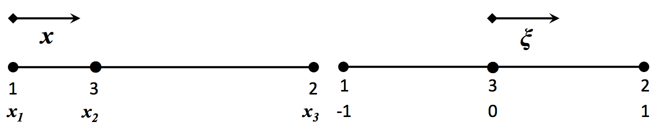
"### Isoparametric Mapping\n",
"\n",
"Based on our choice of the $\\xi_i$, the isoparametric mapping for the quadratic map looks like\n",
"\n",
" \n",
"\n",
"Mathematically, the mapping from physical to natural coordinates is similar in structure to that of the linear element and is given by\n",
"\n",
"\n",
"$$\n",
"x = \\sum_{i=1}^3 N_i(\\xi) x_i \\Longrightarrow\n",
"-\\frac{1}{2}\\xi\\left(1-\\xi\\right)x_1 + \n",
"\\frac{1}{2}\\xi\\left(1+\\xi\\right)x_2 + \n",
"\\left(1-\\xi^2\\right)x_3\n",
"$$\n",
"\n",
"And the Jacobian is given by\n",
"\n",
"$$\n",
"\\begin{align}\n",
"J &= \\frac{dx}{d\\xi} = \\sum_{i=1}^{3} \\frac{dN_i(\\xi)}{d\\xi}x_i \\\\\n",
" &= \\frac{1}{2}\\left(2\\xi - 1\\right)x_1 + \n",
" \\frac{1}{2}\\left(2\\xi + 1\\right)x_2 +\n",
" 2\\xi x_3\n",
"\\end{align}\n",
"$$\n",
"\n",
"Note that the Jacobian is no longer constant and must be included in the integration of the force and stiffness matrices."
]
},
{
"cell_type": "markdown",
"metadata": {},
"source": [
"## Higher Order Lagrange Shape Functions\n",
"\n",
"Higher order Lagrange shape functions are derived similarly to the linear and quadratic."
]
},
{
"cell_type": "markdown",
"metadata": {},
"source": [
"# Example[](#top)"
]
},
{
"cell_type": "code",
"execution_count": null,
"metadata": {
"collapsed": true
},
"outputs": [],
"source": []
}
],
"metadata": {
"kernelspec": {
"display_name": "Python 2",
"language": "python",
"name": "python2"
},
"language_info": {
"codemirror_mode": {
"name": "ipython",
"version": 2
},
"file_extension": ".py",
"mimetype": "text/x-python",
"name": "python",
"nbconvert_exporter": "python",
"pygments_lexer": "ipython2",
"version": "2.7.9"
}
},
"nbformat": 4,
"nbformat_minor": 0
}
\n",
"\n",
"Mathematically, the mapping from physical to natural coordinates is similar in structure to that of the linear element and is given by\n",
"\n",
"\n",
"$$\n",
"x = \\sum_{i=1}^3 N_i(\\xi) x_i \\Longrightarrow\n",
"-\\frac{1}{2}\\xi\\left(1-\\xi\\right)x_1 + \n",
"\\frac{1}{2}\\xi\\left(1+\\xi\\right)x_2 + \n",
"\\left(1-\\xi^2\\right)x_3\n",
"$$\n",
"\n",
"And the Jacobian is given by\n",
"\n",
"$$\n",
"\\begin{align}\n",
"J &= \\frac{dx}{d\\xi} = \\sum_{i=1}^{3} \\frac{dN_i(\\xi)}{d\\xi}x_i \\\\\n",
" &= \\frac{1}{2}\\left(2\\xi - 1\\right)x_1 + \n",
" \\frac{1}{2}\\left(2\\xi + 1\\right)x_2 +\n",
" 2\\xi x_3\n",
"\\end{align}\n",
"$$\n",
"\n",
"Note that the Jacobian is no longer constant and must be included in the integration of the force and stiffness matrices."
]
},
{
"cell_type": "markdown",
"metadata": {},
"source": [
"## Higher Order Lagrange Shape Functions\n",
"\n",
"Higher order Lagrange shape functions are derived similarly to the linear and quadratic."
]
},
{
"cell_type": "markdown",
"metadata": {},
"source": [
"# Example[](#top)"
]
},
{
"cell_type": "code",
"execution_count": null,
"metadata": {
"collapsed": true
},
"outputs": [],
"source": []
}
],
"metadata": {
"kernelspec": {
"display_name": "Python 2",
"language": "python",
"name": "python2"
},
"language_info": {
"codemirror_mode": {
"name": "ipython",
"version": 2
},
"file_extension": ".py",
"mimetype": "text/x-python",
"name": "python",
"nbconvert_exporter": "python",
"pygments_lexer": "ipython2",
"version": "2.7.9"
}
},
"nbformat": 4,
"nbformat_minor": 0
}