 \n",
"\n",
"This lecture by Tim Fuller is licensed under the\n",
"Creative Commons Attribution 4.0 International License. All code examples are also licensed under the [MIT license](http://opensource.org/licenses/MIT)."
]
},
{
"cell_type": "markdown",
"metadata": {},
"source": [
"# Introduction\n",
"\n",
"Using simple axial bar elements and transformation equations we were able to solve for the deformation of a 3D space truss under prescribed load/support conditions.\n",
"\n",
"Using the same connectivity table we were able to solve for the temperature distribution assuming a prescribed temperature at the support and loaded nodes, and neglecting the effect of convection to the surrounds.\n",
"\n",
"In reality, the heat loss to the surrounding air would be significant and should be considered in the design process.\n",
"\n",
"Thermal expansion and self weight may significantly affect the structural response.\n",
"\n",
"
\n",
"\n",
"This lecture by Tim Fuller is licensed under the\n",
"Creative Commons Attribution 4.0 International License. All code examples are also licensed under the [MIT license](http://opensource.org/licenses/MIT)."
]
},
{
"cell_type": "markdown",
"metadata": {},
"source": [
"# Introduction\n",
"\n",
"Using simple axial bar elements and transformation equations we were able to solve for the deformation of a 3D space truss under prescribed load/support conditions.\n",
"\n",
"Using the same connectivity table we were able to solve for the temperature distribution assuming a prescribed temperature at the support and loaded nodes, and neglecting the effect of convection to the surrounds.\n",
"\n",
"In reality, the heat loss to the surrounding air would be significant and should be considered in the design process.\n",
"\n",
"Thermal expansion and self weight may significantly affect the structural response.\n",
"\n",
"\n",
"How can we capture these important thermal and mechanical mechanisms without the cost and complexity of a 3D solid model?\n",
"
"
]
},
{
"cell_type": "markdown",
"metadata": {},
"source": [
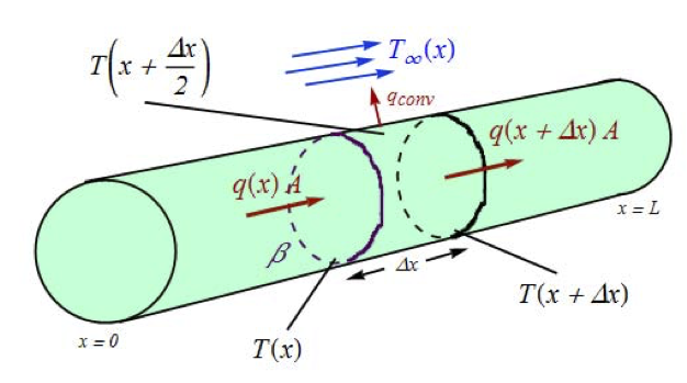
"# Axial Bar with Surface Convection\n",
"\n",
"For the bar shown, two heat transfer mechanisms occur at each point along the bar\n",
"\n",
"\n",
" \n",
" \n",
" | \n",
"\n",
" \n",
" \n",
" | \n",
"
 | \n",
"
\n",
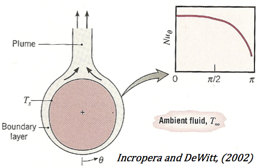
"If large surface temperature variations occur over the structure, this correlation could be used to develop a more accurate model by allowing $h(x)$ to vary with position over an element, otherwise some constant $h_e$ could be computed for each element.\n",
"
\n",
"\n",
"## Strong Form\n",
"\n",
"### Balance Law\n",
"\n",
"At each point, the axial conduction is equal to the conduction out plus the convection to the surroundings.\n",
"\n",
"For some differential length:\n",
"\n",
"$$\n",
"q(x)A(x) - \\beta h\\left(T(x) - T_\\infty(x)\\right)\\Delta x - \n",
" q(x+\\Delta x)A\\left(x+\\Delta x\\right)=0\n",
"$$\n",
"\n",
"Taking the limit as $\\Delta x\\rightarrow 0$, we obtain\n",
"\n",
"$$\n",
"\\beta h\\left(T(x) - T_{\\infty}\\right)+A(x)\\frac{dq}{dx}=0\n",
"$$\n",
"\n",
"### Flux-Potential Relationship\n",
"\n",
"For heat conduction, the flux-potential relationship is modeled by Fourier's law:\n",
"\n",
"$$\n",
"T(x) - T(x+\\Delta x) = q(x)\\frac{\\Delta x}{k_{th}A}\n",
"$$\n",
"\n",
"or, in differential form\n",
"\n",
"$$\n",
"q(x) = -k_{th}\\frac{dT}{dx}\n",
"$$\n",
"\n",
"Substituting the flux potential relationship into the balance law we obtain the **strong form** for axial conduction in a bar with surface convection\n",
"\n",
"$$\n",
"k_{th}A(x)\\frac{d^2T}{dx^2}-\\beta h T\\left(T(x)-T_{\\infty}\\right)=0, \\quad 0 \\leq x \\leq L\n",
"$$\n",
"\n",
"with Dirichlet boundary conditions\n",
"\n",
"$$\n",
"T(0) = T_h, \\quad T(L) = T_c\n",
"$$"
]
},
{
"cell_type": "markdown",
"metadata": {},
"source": [
"## Weak Form\n",
"\n",
"Assuming the problem data (what are all the problem data?) are constant, the strong form is\n",
"\n",
"$$\n",
"kAT''-\\beta h\\left(T-T_{\\infty}\\right)=0, \\quad 0 \\leq x \\leq L\n",
"$$\n",
"$$\n",
"T(0) = T_h, \\quad T(L) = T_c\n",
"$$\n",
"\n",
"Following the 3 step procedure\n",
"\n",
"1. Multiply by a weight function and integrate over the domain\n",
"$$\n",
"\\int_0^L w\\left(\n",
"kAT''-\\beta h\\left(T-T_{\\infty}\\right)\\right)dx = 0 \\quad \\forall w\n",
"$$\n",
"2. Integrate by parts\n",
"$$\n",
"-\\int_0^L w'kAT'-\\beta h\\left(T-T_{\\infty}\\right)dx\n",
"+kAwT'\\Bigg|_0^L\n",
"$$\n",
"3. Enforce essential boundary conditions\n",
"$$\n",
"kAwT'\\Bigg|_0^L=kAw(L)T'(L)-kAw(0)T'(0)=0, \\quad \\forall w\n",
"$$\n",
"\n",
"So, the weak form for axial conduction in a bar with surface convection and Dirichlet boundaries is\n",
"\n",
"$$\n",
"\\int_0^L w'kAT'dx + \n",
"\\int_0^L\\beta hTdx -\n",
"\\int_0^L\\beta hT_{\\infty}dx=0, \\quad\n",
"\\forall w, \\ w(0) = w(L) = 0\n",
"$$"
]
},
{
"cell_type": "markdown",
"metadata": {},
"source": [
"# Approximate Solution\n",
"\n",
"Express the integral over the domain as a sum of integrals over elements\n",
"\n",
"$$ \\begin{multline}\n",
"\\sum_e \\left(\n",
"\\int_{x_0^{(e)}}^{x_L^{(e)}} {w^{(e)}}' k^{(e)}A^{(e)} {T^{(e)}}' dx + \n",
"\\int_{x_0^{(e)}}^{x_L^{(e)}} w^{(e)} \\beta^{(e)} h^{(e)} T^{(e)} dx - \\\\\n",
"\\int_{x_0^{(e)}}^{x_L^{(e)}} w^{(e)} \\beta^{(e)} h^{(e)} T_{\\infty} dx\n",
"\\right)=0, \\quad\n",
"\\forall w, \\ w(0) = w(L) = 0\n",
"\\end{multline} $$\n",
"\n",
"Introduce an approximation for the \"trial\" solution and weight \"test\" function\n",
"\n",
"$$\n",
"T^e = N_i^e T_i^e, \\quad\n",
"\\frac{dT^e}{dx} = \\frac{dN_i^e}{dx}T_i^e = B_i^eT_i^e, \\quad\n",
"w^e = w_i^eN_i^e, \\quad\n",
"\\frac{dw^e}{dx} = w_i^e\\frac{dN_i^e}{dx}\n",
"$$\n",
"\n",
"Substituting in to the weak form gives\n",
"\n",
"$$\n",
"\\begin{multline}\n",
"\\sum_e\\left(\\int_{x_0^{(e)}}^{x_L^{(e)}} w_i^{(e)}\\frac{dN_i^{(e)}}{dx}k^{(e)}A^{(e)}\\frac{dN_j^{(e)}}{dx} T_j^{(e)} +\n",
"\\int_{x_0^{(e)}}^{x_L^{(e)}} w_i^{(e)}N_i^{(e)}\\beta^{(e)} h^{(e)} N_j^{(e)}T_j^{(e)}dx \\right. \\\\ \\left. -\n",
"\\int_{x_0^{(e)}}^{x_L^{(e)}} w_i^{(e)}N_i^{(e)} \\beta^{(e)} h^{(e)} T_{\\infty}dx\\right)=0, \\quad\n",
"\\forall w, \\ w_1 = w_n = 0\n",
"\\end{multline}\n",
"$$\n",
"\n",
"We factor out the $w_i^{(e)}$ of each term and rearrange\n",
"\n",
"$$\n",
"\\begin{multline}\n",
"\\sum_ew_i^{(e)}\\left[\n",
"\\left(\n",
"\\int_{x_0^{(e)}}^{x_L^{(e)}} k^{(e)}A^{(e)}\\frac{dN_i^{(e)}}{dx}\\frac{dN_j^{(e)}}{dx} +\n",
"\\int_{x_0^{(e)}}^{x_L^{(e)}} \\beta^{(e)} h^{(e)} N_i^{(e)} N_j^{(e)}dx\\right)T_j^{(e)} \\right.\\\\\n",
"\\left.-\n",
"\\int_{x_0^{(e)}}^{x_L^{(e)}} \\beta^{(e)} h^{(e)} N_i^{(e)} T_{\\infty}dx\\right] = 0, \\quad\n",
"\\forall w, \\ w_1 = w_n = 0\n",
"\\end{multline}\n",
"$$\n",
"\n",
"Writing this in a more compact form\n",
"\n",
"$$\n",
"\\sum_e w_i^{(e)} \\left(k_{ij}^{(e)}T_j^{(e)} - f_i^{(e)}\\right) = 0\n",
"$$\n",
"\n",
"where the stiffness $k_{ij}^{(e)}$ is\n",
"\n",
"$$\n",
"k_{ij}^{(e)}=\\int_{x_0^{(e)}}^{x_L^{(e)}} k^{(e)}A^{(e)}\\frac{dN_i^{(e)}}{dx}\\frac{dN_j^{(e)}}{dx} +\n",
"\\int_{x_0^{(e)}}^{x_L^{(e)}} \\beta^{(e)} h^{(e)} N_i^{(e)} N_j^{(e)}dx\n",
"$$\n",
"\n",
"and the **element external flux array**, (equivalent to the force array for our structural problem), which is a sum of boundary and body forces\n",
"\n",
"$$\n",
"f_i^{(e)} = f_{\\Gamma i}^{(e)} + f_{\\Omega i}^{(e)} = \n",
"\\int_{x_0^{(e)}}^{x_L^{(e)}} \\beta^{(e)} h^{(e)} N_i^{(e)} T_{\\infty}dx\n",
"$$\n",
"\n",
"For this problem the boundary source array is zero, as we have specified Dirichlet boundaries at each end of the domain. This is often done in discussion of FE when the focus is the development of an element stiffness matrix. We have not yet specified the function $T_{\\infty}$ that determines how the free stream temperature varies along the bar."
]
},
{
"cell_type": "markdown",
"metadata": {
"collapsed": true
},
"source": [
"# Thermal Stresses\n",
"\n",
"From the temperature distribution in the truss members, we can compute the thermal expansion strains to see how these affect the stresses and displacements in the structure.\n",
"\n",
"**Strong Form**\n",
"\n",
"$$\n",
"\\frac{d}{dx}\\left(EA(x)\\frac{du}{dx}-E\\alpha A(x) T(x)\\right) = 0\n",
"$$\n",
"\n",
"**Weak Form**\n",
"\n",
"$$\n",
"\\int_0^Lw'(x) EA u'(x) dx + \\int_0^L w(x) EA\\alpha T'(x) dx = 0, \\quad\n",
"\\forall w(x), w(x)_{x=0,L}=0\n",
"$$\n",
"\n",
"**Finite Element Equations**\n",
"\n",
"$$\n",
"k_{ij}^{(e)}u_j^{(e)} - f_i^{(e)} = 0\n",
"$$\n",
"\n",
"where\n",
"\n",
"$$\n",
"k_{ij}^{(e)} = \\int_{x_0^{(e)}}^{x_L^{(e)}}\n",
"A^{(e)}E^{(e)}\\frac{dN_i}{dx}\\frac{dN_j}{dx} dx\n",
"$$\n",
"\n",
"$$\n",
"f_i^{(e)} = -\\int_{x_0^{(e)}}^{x_L^{(e)}}N_i^{(e)}(x)EA\\alpha\\frac{dT^{(e)}}{dx}dx\n",
"$$\n",
"\n",
"The thermal stresses appear in the form of a body force, adding a force that counteracts that normally required to achieve some amount of thermal expansion.\n",
"\n",
"\n",
"Thus, we see that thermal effects can be readily added to an existing model, through the addition of force terms. This approach can be used to model all types of zero‐stress deformation mechanics such as curing or drying of composites, water absorption, etc.\n",
"
"
]
},
{
"cell_type": "markdown",
"metadata": {},
"source": [
"# Exercises\n",
"\n",
"## Exercise 1 [60]\n",
"\n",
"Modified from Fish & Belytschko, Problem 5.1\n",
"For this problem do NOT use the direct stiffness method.\n",
"\n",
"Consider a heat conduction problem in the domain [0, 20]m. The bar has a unit cross section, constant thermal conductivity $k=5$W/$^{\\text{o}}C$$\\cdot$m and a uniform heat source $s=100$ W/m. The boundary conditions are $T(0)=0^{\\text{o}}C$ and $\\overline{q}(20)=0$W/m$^2$. Solve the problem with two equal linear elements. Plot the finite element solution $T_N(x)$ and $dT_N(x)/dx$ and compare to the exact solution which is given by $T(x)=-10x^2+400x$."
]
},
{
"cell_type": "markdown",
"metadata": {},
"source": [
"## Exercise 2\n",
"\n",
" \n",
"\n",
"For the bar shown,\n",
"\n",
"a) State the strong form representing heat flow and solve analytically. Give the symbolic solution $T(x)$ and total heat flux $Q(x)$ along the length of the bar.\n",
"\n",
"b) Construct the element body source arrays, the boundary force arrays, and assemble the global external force array.\n",
"\n",
"c) Construct the element stiffness matrices and assemble the global stiffness matrix.\n",
"\n",
"d) Solve for the temperature distribution $T(x)$. Generate a plot of the global approximate solution $T_N(x)$ along the length of the bar overlaid with the analytic solution."
]
}
],
"metadata": {
"kernelspec": {
"display_name": "Python 2",
"language": "python",
"name": "python2"
},
"language_info": {
"codemirror_mode": {
"name": "ipython",
"version": 2
},
"file_extension": ".py",
"mimetype": "text/x-python",
"name": "python",
"nbconvert_exporter": "python",
"pygments_lexer": "ipython2",
"version": "2.7.9"
}
},
"nbformat": 4,
"nbformat_minor": 0
}
\n",
"\n",
"For the bar shown,\n",
"\n",
"a) State the strong form representing heat flow and solve analytically. Give the symbolic solution $T(x)$ and total heat flux $Q(x)$ along the length of the bar.\n",
"\n",
"b) Construct the element body source arrays, the boundary force arrays, and assemble the global external force array.\n",
"\n",
"c) Construct the element stiffness matrices and assemble the global stiffness matrix.\n",
"\n",
"d) Solve for the temperature distribution $T(x)$. Generate a plot of the global approximate solution $T_N(x)$ along the length of the bar overlaid with the analytic solution."
]
}
],
"metadata": {
"kernelspec": {
"display_name": "Python 2",
"language": "python",
"name": "python2"
},
"language_info": {
"codemirror_mode": {
"name": "ipython",
"version": 2
},
"file_extension": ".py",
"mimetype": "text/x-python",
"name": "python",
"nbconvert_exporter": "python",
"pygments_lexer": "ipython2",
"version": "2.7.9"
}
},
"nbformat": 4,
"nbformat_minor": 0
}