 \n",
"\n",
"
\n",
"\n",
" \n",
"\n",
"This lecture by Tim Fuller is licensed under the\n",
"Creative Commons Attribution 4.0 International License. All code examples are also licensed under the [MIT license](http://opensource.org/licenses/MIT)."
]
},
{
"cell_type": "markdown",
"metadata": {},
"source": [
"# Topics\n",
"\n",
"- [Introduction](#intro)\n",
"- [Sources of Error](#sources)\n",
"- [Error Metrics](#metrics)\n",
"- [Convergence](#convergence)\n",
"- [Solution Accuracy](#accuracy)\n",
"- [Methods of Error Estimation](#methods)\n",
" - [Richardson's Extrapolation](#rich)\n",
"- [Error Estimation Procedures](#proc)\n",
"- [Error Estimation Example](#example)"
]
},
{
"cell_type": "markdown",
"metadata": {},
"source": [
"# Introduction[
\n",
"\n",
"This lecture by Tim Fuller is licensed under the\n",
"Creative Commons Attribution 4.0 International License. All code examples are also licensed under the [MIT license](http://opensource.org/licenses/MIT)."
]
},
{
"cell_type": "markdown",
"metadata": {},
"source": [
"# Topics\n",
"\n",
"- [Introduction](#intro)\n",
"- [Sources of Error](#sources)\n",
"- [Error Metrics](#metrics)\n",
"- [Convergence](#convergence)\n",
"- [Solution Accuracy](#accuracy)\n",
"- [Methods of Error Estimation](#methods)\n",
" - [Richardson's Extrapolation](#rich)\n",
"- [Error Estimation Procedures](#proc)\n",
"- [Error Estimation Example](#example)"
]
},
{
"cell_type": "markdown",
"metadata": {},
"source": [
"# Introduction[ ](#top)\n",
"\n",
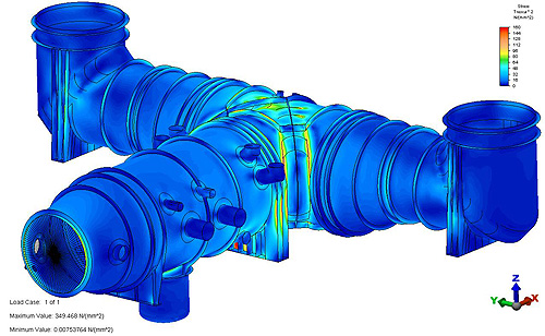
"In the finite element method, as in any approximation method, there will also be some error associated with your approximate solution. Quantifying that error so that you can have confidence in your answer is an important part of finite element analysis and is the subject of these notes."
]
},
{
"cell_type": "markdown",
"metadata": {},
"source": [
"# Sources of Error[](#top)\n",
"\n",
"The errors to the solution of a differential equation found using the FEM can be attributed to three basic sources:\n",
"\n",
"- Domain Approximation Error\n",
"\n",
"In the 1D problems we have discussed so far this semester, the domains have been considered straight lines, therefore, no approximation of the domain has been necessary. In 2D and 3D problems, involving non-rectangular domains, boundary approximation errors are introduced into the finite element solutions. How are these errors interpreted? In general, we can think of them as errors in the specification of the problem data because we are now solving the DE on a modified domain. This error can be reduced by refining the mesh.\n",
"\n",
"- Quadrature and Finite Arithmetic Errors\n",
"\n",
"When FE computations are performed on a computer, round-off errors in the computation of numbers and errors due to the numerical evaluation of integrals are introduced into the solution. For linear problems, with a reasonably small number of degrees of freedom, this error is generally quite small.\n",
"\n",
"- Approximation Error\n",
"\n",
"The error introduced into the finite element solution ${U_N}^{(e)}$ because of the approximation of the dependent variable $u$ in an element $\\Omega^{(e)}$ is inherent to any problem\n",
"\n",
"$$\n",
"u\\approx U_N = \\sum_{e=1}^N\\sum_{i=1}^nu_i^{(e)}N_i^{(e)}=\\sum_{I=1}^Mu_I\\Phi_I\n",
"$$\n",
"\n",
"where $u_I$ is the value of $u$ at the global node $I$, $\\Phi_I$ is the global interpolation function associated with global node $I$, $U_N$ is the finite element solution over the domain, $N$ is the number of elements in the mesh, $M$ is the total number of global nodes, and $n$ is the number of nodes in an element.\n",
"\n",
"We wish to quantify the error $E=u-U_N$ and know how the error changes with $n$ and $M$."
]
},
{
"cell_type": "markdown",
"metadata": {},
"source": [
"# Error Metrics[](#top)\n",
"\n",
"The error metrics that we will be considering today fall into the category of \"norms\". The norm of a mathematical object, from [Wolfram MathWorld](http://mathworld.wolfram.com/Norm.html), is a quantity that in some (possibly abstract) sense describes the length, size, or extent of the object. The norm of an object $x$ will be denoted by $\\lVert x \\rVert$.\n",
"\n",
"Let $U_N$ be an approximation for $u$. The ``energy-norm'' error of the approximation over a range form $x=a$ to $x=b$ is \n",
"$$\n",
"\\lVert u-U_N \\rVert_m=\\left[\n",
"\\int_a^b\\sum_{i=0}^m\\left(\\frac{d^iu}{dx^i}-\\frac{d^iU_N}{dx^i}\\right)^2\\,dx\n",
"\\right]^{1/2}\n",
"$$\n",
"where $2m$ is the order of the differential equation being solved. The term \"energy-norm\" is used to indicate that this norm contains the same order derivatives as the quadratic functional associated with the equation, which, for most solid mechanics problems, denotes the energy.\n",
"\n",
"The \"p-norm\" is\n",
"$$\n",
"L_p=\\left[\\int_a^b\\left( u-U_N\\right)^p\\,dx\\right]^{1/p}\n",
"$$\n",
"\n",
"The $L_2$ norm is the most commonly used p-norm and is given by\n",
"$$\n",
"\\lVert u-U_N \\rVert_0=\\left[\n",
"\\int_a^b\\left( u-U_N \\right)^2\\,dx\n",
"\\right]^{1/2}\n",
"$$\n",
"\n",
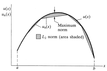
"The \"maximum-norm\" is defined to be the the maximum of all absolute values of the differences of $u$ and $U_N$ in the domain $\\Omega=(a,b)$:\n",
"$$\n",
"\\lVert u - U_N\\rVert_{\\infty}=\\stackrel{\\text{max}}{ \\scriptstyle a\\leq x\\leq b} \\ \\lvert u(x)-U_N(x) \\rvert\n",
"$$\n",
"\n",
"The $L_2$ norm and maximum norm error metric are illustrated in below\n",
"\n",
"
](#top)\n",
"\n",
"In the finite element method, as in any approximation method, there will also be some error associated with your approximate solution. Quantifying that error so that you can have confidence in your answer is an important part of finite element analysis and is the subject of these notes."
]
},
{
"cell_type": "markdown",
"metadata": {},
"source": [
"# Sources of Error[](#top)\n",
"\n",
"The errors to the solution of a differential equation found using the FEM can be attributed to three basic sources:\n",
"\n",
"- Domain Approximation Error\n",
"\n",
"In the 1D problems we have discussed so far this semester, the domains have been considered straight lines, therefore, no approximation of the domain has been necessary. In 2D and 3D problems, involving non-rectangular domains, boundary approximation errors are introduced into the finite element solutions. How are these errors interpreted? In general, we can think of them as errors in the specification of the problem data because we are now solving the DE on a modified domain. This error can be reduced by refining the mesh.\n",
"\n",
"- Quadrature and Finite Arithmetic Errors\n",
"\n",
"When FE computations are performed on a computer, round-off errors in the computation of numbers and errors due to the numerical evaluation of integrals are introduced into the solution. For linear problems, with a reasonably small number of degrees of freedom, this error is generally quite small.\n",
"\n",
"- Approximation Error\n",
"\n",
"The error introduced into the finite element solution ${U_N}^{(e)}$ because of the approximation of the dependent variable $u$ in an element $\\Omega^{(e)}$ is inherent to any problem\n",
"\n",
"$$\n",
"u\\approx U_N = \\sum_{e=1}^N\\sum_{i=1}^nu_i^{(e)}N_i^{(e)}=\\sum_{I=1}^Mu_I\\Phi_I\n",
"$$\n",
"\n",
"where $u_I$ is the value of $u$ at the global node $I$, $\\Phi_I$ is the global interpolation function associated with global node $I$, $U_N$ is the finite element solution over the domain, $N$ is the number of elements in the mesh, $M$ is the total number of global nodes, and $n$ is the number of nodes in an element.\n",
"\n",
"We wish to quantify the error $E=u-U_N$ and know how the error changes with $n$ and $M$."
]
},
{
"cell_type": "markdown",
"metadata": {},
"source": [
"# Error Metrics[](#top)\n",
"\n",
"The error metrics that we will be considering today fall into the category of \"norms\". The norm of a mathematical object, from [Wolfram MathWorld](http://mathworld.wolfram.com/Norm.html), is a quantity that in some (possibly abstract) sense describes the length, size, or extent of the object. The norm of an object $x$ will be denoted by $\\lVert x \\rVert$.\n",
"\n",
"Let $U_N$ be an approximation for $u$. The ``energy-norm'' error of the approximation over a range form $x=a$ to $x=b$ is \n",
"$$\n",
"\\lVert u-U_N \\rVert_m=\\left[\n",
"\\int_a^b\\sum_{i=0}^m\\left(\\frac{d^iu}{dx^i}-\\frac{d^iU_N}{dx^i}\\right)^2\\,dx\n",
"\\right]^{1/2}\n",
"$$\n",
"where $2m$ is the order of the differential equation being solved. The term \"energy-norm\" is used to indicate that this norm contains the same order derivatives as the quadratic functional associated with the equation, which, for most solid mechanics problems, denotes the energy.\n",
"\n",
"The \"p-norm\" is\n",
"$$\n",
"L_p=\\left[\\int_a^b\\left( u-U_N\\right)^p\\,dx\\right]^{1/p}\n",
"$$\n",
"\n",
"The $L_2$ norm is the most commonly used p-norm and is given by\n",
"$$\n",
"\\lVert u-U_N \\rVert_0=\\left[\n",
"\\int_a^b\\left( u-U_N \\right)^2\\,dx\n",
"\\right]^{1/2}\n",
"$$\n",
"\n",
"The \"maximum-norm\" is defined to be the the maximum of all absolute values of the differences of $u$ and $U_N$ in the domain $\\Omega=(a,b)$:\n",
"$$\n",
"\\lVert u - U_N\\rVert_{\\infty}=\\stackrel{\\text{max}}{ \\scriptstyle a\\leq x\\leq b} \\ \\lvert u(x)-U_N(x) \\rvert\n",
"$$\n",
"\n",
"The $L_2$ norm and maximum norm error metric are illustrated in below\n",
"\n",
" \n",
"\n",
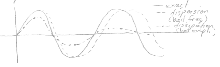
"The $L_2$ norm is the most commonly used error metric, but there are many others. If, for example, you are studying vibrations, then you might seek alternative quantifiers of dispersion and dissipation (the $L_2$ norm is misleading in these problems):\n",
"\n",
"
\n",
"\n",
"The $L_2$ norm is the most commonly used error metric, but there are many others. If, for example, you are studying vibrations, then you might seek alternative quantifiers of dispersion and dissipation (the $L_2$ norm is misleading in these problems):\n",
"\n",
" "
]
},
{
"cell_type": "markdown",
"metadata": {},
"source": [
"# Convergence[](#top)\n",
"\n",
"The finite element solution $U_N$ is said to *em converge in the energy norm* norm to the true solution $u$ if\n",
"\n",
"$$\n",
"\\lVert u-U_N \\rVert_m \\leq ch^p \\ \\text{ for } p>0\n",
"$$\n",
"\n",
"where $c$ is a constant independent of $u$ and $U_N$, and $h$ is the characteristic length of an element. The constant $p$ is called the rate of convergence. Note that the convergence depends on $h$ as well as on $p$; $p$ depends on the order of the derivative of $u$ in the weak form and the degree of the polynomials used to approximate $u$. Therefore, the error in the approximation can be reduced either by reducing the size of the elements or increasing the degree of approximation. Convergence of the finite element solutions with mesh refinements is termed *h-convergence*. Convergence with increasing degree of polynomials is called *p-convergence*.\n",
"\n",
"In ANSYS, both $h$-Elements and $p$-Elements are available. The $h$-Element is the traditional element that we have been using and greater accuracy can be achieved using mesh refinement. The $p$-Element uses a constant mesh and varies the degree of the polynomial to obtain the results to a user specified accuracy. Each type of element has its advantages and disadvantages."
]
},
{
"cell_type": "markdown",
"metadata": {},
"source": [
"# Accuracy of the Solution[](#top)\n",
"\n",
"If the finite element interpolation functions $\\Phi_i$ are complete polynomials of degree $k$, then the error in the $L_p$ norm can be shown to satisfy the inequality\n",
"\n",
"$$\n",
"\\lVert e \\rVert_m = \\lVert u-U_N \\rVert_m\\leq ch^p, \\quad p=k+1-m\n",
"$$\n",
"\n",
"where $c$ is a constant. This estimate implies that the error goes to zero as the $p^{\\text{th}}$ power of $h$ as $h$ is decreased.\n",
"\n",
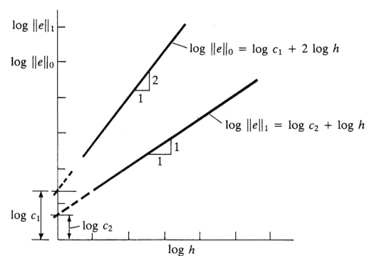
"How can we use this relationship to make judgements about our approximate solution, even if the true solution is not known? Let us take the $\\log$ of both sides\n",
"\n",
"$$\n",
"\\log{\\lVert e \\rVert_m}=\\log{c}+p\\log{h}\n",
"$$\n",
"\n",
"We see that the logarithm of the error in the energy norm versus the logarithm of $h$ is a straight line whose slope is $p$ and intercept is $\\log{c}$. The greater the degree of the interpolation functions, the more rapid the rate of convergence (because $p \\propto k$). Note that the error in the energy goes to zero at the rate of $k+1-m$; the error in the $L_2$ norm will decrease even more rapidly, namely, at the rate of $k+1$, i.e., derivatives converge more slowly than the solution itself. \n",
"\n",
"Error estimates of this type are very useful because they give an idea of the accuracy of the approximate solution, whether or not we know the true solution. While the estimate gives an idea of how rapidly the finite element solution converges to the true solution, it does not tell us when to stop refining the mesh. This decision is up to the analyst who presumably knows what a reasonable tolerance is for the problem being solved."
]
},
{
"cell_type": "markdown",
"metadata": {},
"source": [
"# Error Estimation Methods[](#top)\n",
"\n",
"*A posteriori* error estimates can roughly be divided into four categories\n",
"\n",
"1. *Residual error estimates*. Local finite element problems are created on either an element or a subdomain and solved for the error estimate. The data depends on the residual of the finite element solution.\n",
"\n",
"2. *Flux-projection error estimates*. A new flux is calculated by post processing the finite element solution. This flux is smoother than the original finite element flux and an error estimate is obtained from the difference of the two fluxes.\n",
"\n",
"3. *Extrapolation error estimates*. Two finite element solutions having different orders or different meshes are compared and their differences used to provide an error estimate.\n",
"\n",
"4. *Interpolation error estimates*. Interpolation error bounds are used with estimates of the unknown constants."
]
},
{
"cell_type": "markdown",
"metadata": {},
"source": [
"## Richardson's Extrapolation\n",
"\n",
"
"
]
},
{
"cell_type": "markdown",
"metadata": {},
"source": [
"# Convergence[](#top)\n",
"\n",
"The finite element solution $U_N$ is said to *em converge in the energy norm* norm to the true solution $u$ if\n",
"\n",
"$$\n",
"\\lVert u-U_N \\rVert_m \\leq ch^p \\ \\text{ for } p>0\n",
"$$\n",
"\n",
"where $c$ is a constant independent of $u$ and $U_N$, and $h$ is the characteristic length of an element. The constant $p$ is called the rate of convergence. Note that the convergence depends on $h$ as well as on $p$; $p$ depends on the order of the derivative of $u$ in the weak form and the degree of the polynomials used to approximate $u$. Therefore, the error in the approximation can be reduced either by reducing the size of the elements or increasing the degree of approximation. Convergence of the finite element solutions with mesh refinements is termed *h-convergence*. Convergence with increasing degree of polynomials is called *p-convergence*.\n",
"\n",
"In ANSYS, both $h$-Elements and $p$-Elements are available. The $h$-Element is the traditional element that we have been using and greater accuracy can be achieved using mesh refinement. The $p$-Element uses a constant mesh and varies the degree of the polynomial to obtain the results to a user specified accuracy. Each type of element has its advantages and disadvantages."
]
},
{
"cell_type": "markdown",
"metadata": {},
"source": [
"# Accuracy of the Solution[](#top)\n",
"\n",
"If the finite element interpolation functions $\\Phi_i$ are complete polynomials of degree $k$, then the error in the $L_p$ norm can be shown to satisfy the inequality\n",
"\n",
"$$\n",
"\\lVert e \\rVert_m = \\lVert u-U_N \\rVert_m\\leq ch^p, \\quad p=k+1-m\n",
"$$\n",
"\n",
"where $c$ is a constant. This estimate implies that the error goes to zero as the $p^{\\text{th}}$ power of $h$ as $h$ is decreased.\n",
"\n",
"How can we use this relationship to make judgements about our approximate solution, even if the true solution is not known? Let us take the $\\log$ of both sides\n",
"\n",
"$$\n",
"\\log{\\lVert e \\rVert_m}=\\log{c}+p\\log{h}\n",
"$$\n",
"\n",
"We see that the logarithm of the error in the energy norm versus the logarithm of $h$ is a straight line whose slope is $p$ and intercept is $\\log{c}$. The greater the degree of the interpolation functions, the more rapid the rate of convergence (because $p \\propto k$). Note that the error in the energy goes to zero at the rate of $k+1-m$; the error in the $L_2$ norm will decrease even more rapidly, namely, at the rate of $k+1$, i.e., derivatives converge more slowly than the solution itself. \n",
"\n",
"Error estimates of this type are very useful because they give an idea of the accuracy of the approximate solution, whether or not we know the true solution. While the estimate gives an idea of how rapidly the finite element solution converges to the true solution, it does not tell us when to stop refining the mesh. This decision is up to the analyst who presumably knows what a reasonable tolerance is for the problem being solved."
]
},
{
"cell_type": "markdown",
"metadata": {},
"source": [
"# Error Estimation Methods[](#top)\n",
"\n",
"*A posteriori* error estimates can roughly be divided into four categories\n",
"\n",
"1. *Residual error estimates*. Local finite element problems are created on either an element or a subdomain and solved for the error estimate. The data depends on the residual of the finite element solution.\n",
"\n",
"2. *Flux-projection error estimates*. A new flux is calculated by post processing the finite element solution. This flux is smoother than the original finite element flux and an error estimate is obtained from the difference of the two fluxes.\n",
"\n",
"3. *Extrapolation error estimates*. Two finite element solutions having different orders or different meshes are compared and their differences used to provide an error estimate.\n",
"\n",
"4. *Interpolation error estimates*. Interpolation error bounds are used with estimates of the unknown constants."
]
},
{
"cell_type": "markdown",
"metadata": {},
"source": [
"## Richardson's Extrapolation\n",
"\n",
" \n",
"\n",
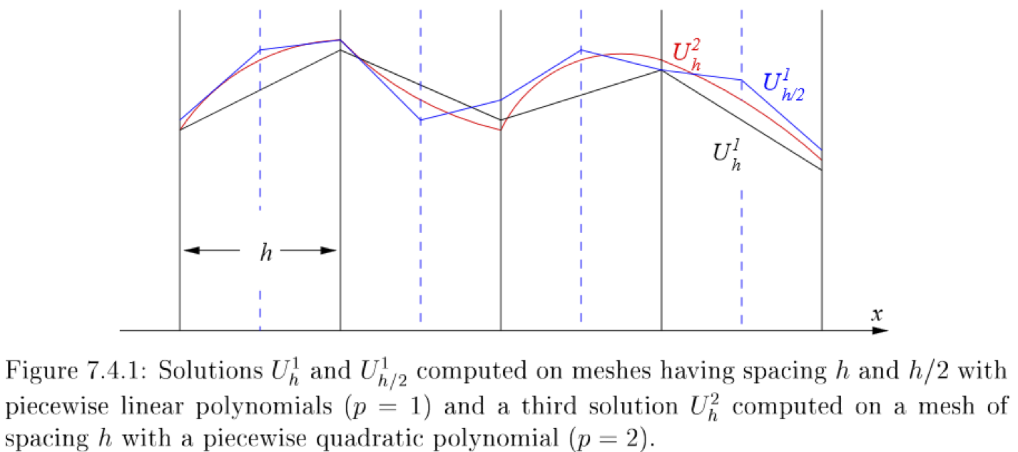
"The four techniques are not independent but have many similarities. Surveys of error estimation procedures describe many of their properties, similarities, and differences. Let us set the stage by briefly describing two simple extrapolation techniques. Consider a one-dimension problem for simplicity and suppose that an approximate solution $U_h^P(x)$ has been computed using a polynomial approximation of degree $p$ on a mesh of spacing $h$, as shown above. Suppose that we have an *a priori* interpolation error estimate of the form\n",
"\n",
"$$\n",
"u(x) - U_h^p(x) = C_{p+1}h^{p+1}+\\mathscr{O}\\left(h^{p+2}\\right)\n",
"$$\n",
"\n",
"We have assumed that the exact solution $u(x)$ is smooth enough for the error to be expanded in $h$ to $\\mathscr{O}\\left(h^{p+2}\\right)$. The leading error constant $C_{p+1}$ generally depends on (unknown) derivatives of $u$. Now, compute a second solution with spacing $h/2$ to obtain\n",
"\n",
"$$\n",
"u(x) - U_{h/2}^p(x) = C_{p+1}\\left(\\frac{h}{2}\\right)^{p+1}+\\mathscr{O}\\left(h^{p+2}\\right)\n",
"$$\n",
"\n",
"Subtracting the two solutions we eliminate the unkown exact solution and obtain\n",
"\n",
"$$\n",
"U_{h/2}^p(x) - U_{h}^p(x) = C_{p+1}h^{p+1}\\left(1-\\frac{1}{2^p+1}\\right)\\mathscr{O}\\left(h^{p+2}\\right)\n",
"$$\n",
"\n",
"Neglecting the higher-order therms, we obtain an approximation of the discretization error as\n",
"\n",
"$$\n",
"C_{p+1}h^{p+1} \\approx\n",
"\\frac{U_{h/2}^p(x) - U_{h}^p(x)}{1-1/2^{p+1}}\n",
"$$\n",
"\n",
"The technique is called *Richardson's extrapolation* or *h-extrapolation*. It can also be used to obtain error estimates of the fine-mesh solution. The cost of obtaining the error estimate is approximately twice the cost of obtaining the solution. In two and three dimensions the cost factors rist to, respectively, four and eight times the solution cost. Most would consider this to be excessive. The only way of justifying the procedure is to consider the fine mesh solution as being the result and the coarse mesh solution as furnishing the error estimate. This strategy only furnishes an error estimate on the coarse mesh."
]
},
{
"cell_type": "markdown",
"metadata": {},
"source": [
"# Error Estimation Procedures[](#top)\n",
"\n",
"It has been shown that the element size affects the accuracy of your results, but how do we know whether the element sizes associated with a meshed model are fine enough to produce good results? A simple way to find out is to first model a problem with a certain number of elements and then compare its results to the results of a model with twice as many elements. If no significant difference between the results of the two meshes is detected, then the meshing is probably alright. If substantially different results are obtained, then further mesh refinement might be necessary."
]
},
{
"cell_type": "markdown",
"metadata": {},
"source": [
"# Error Analysis Example[](#top)\n",
"\n",
"Consider the differential equation\n",
"\n",
"$$\n",
"\\frac{d^2u}{dx^2} + 2 = 0, \\quad x\\in(0,1)\n",
"$$\n",
"\n",
"subject to\n",
"\n",
"$$\n",
"u(0)=u(1)=0\n",
"$$\n",
"\n",
"The exact solution is given by\n",
"\n",
"$$\n",
"u(x)=x(1-x)\n",
"$$\n",
"\n",
"The finite element solutions are given by\n",
"\n",
"$N=2$\n",
"$$\n",
"U_N = \\begin{cases} \n",
"h^2\\left(\\frac{x}{h}\\right) & \\text{for } 0 \\leq x \\leq h \\\\ \n",
"h^2\\left( 2-\\frac{x}{h}\\right) & \\text{for } h \\leq x \\leq 2h\n",
"\\end{cases}\n",
"$$\n",
"\n",
"$N=3$\n",
"$$\n",
"U_N = \\begin{cases}\n",
"2h^2\\left(\\frac{x}{h}\\right) & \\text{for } 0\\leq x \\leq h \\\\ \n",
"2h^2\\left( 2-\\frac{x}{h}\\right) + 2h^2\\left(\\frac{x}{h}-1\\right) & \\text{for } h \\leq x \\leq 2h \\\\ \n",
"2h^2\\left( 3-\\frac{x}{h}\\right) & \\text{for } \\ 2h\\leq x \\leq 3h\n",
"\\end{cases}\n",
"$$\n",
"\n",
"$N=4$\n",
"$$\n",
"U_N = \\begin{cases}\n",
"3h^2\\left(\\frac{x}{h}\\right) & \\text{for } 0\\leq x \\leq h \\\\ \n",
"3h^2\\left( 2-\\frac{x}{h}\\right) + 4h^2\\left(\\frac{x}{h}-1\\right) & \\text{for } h\\leq x \\leq 2h\\\\ \n",
"4h^2\\left(3-\\frac{x}{h}\\right) + 3h^2\\left(\\frac{x}{h}-2\\right) & \\text{for } \\ 2h\\leq x \\leq 3h \\\\ \n",
"3h^2\\left( 4-\\frac{x}{h}\\right) & \\text{for } \\ 3h\\leq x \\leq 4h \\end{cases}\n",
"$$\n",
"\n",
"For the two element case ($h=0.5$), the $L_2$ norm error is given by\n",
"\n",
"$$\n",
"\\lVert u-U_N\\rVert_2^2=\\int_0^{.5}(x-x^2-hx)^2\\,dx+\\int_{.5}^{1}(x-x^2-2h^2+xh)^2\\,dx=0.002083\n",
"$$\n",
"\n",
"Similar calculations can be performed for $N=3$ and $N=4$. The errors for all three cases are shown in the table below:\n",
"\n",
"
\n",
"\n",
"The four techniques are not independent but have many similarities. Surveys of error estimation procedures describe many of their properties, similarities, and differences. Let us set the stage by briefly describing two simple extrapolation techniques. Consider a one-dimension problem for simplicity and suppose that an approximate solution $U_h^P(x)$ has been computed using a polynomial approximation of degree $p$ on a mesh of spacing $h$, as shown above. Suppose that we have an *a priori* interpolation error estimate of the form\n",
"\n",
"$$\n",
"u(x) - U_h^p(x) = C_{p+1}h^{p+1}+\\mathscr{O}\\left(h^{p+2}\\right)\n",
"$$\n",
"\n",
"We have assumed that the exact solution $u(x)$ is smooth enough for the error to be expanded in $h$ to $\\mathscr{O}\\left(h^{p+2}\\right)$. The leading error constant $C_{p+1}$ generally depends on (unknown) derivatives of $u$. Now, compute a second solution with spacing $h/2$ to obtain\n",
"\n",
"$$\n",
"u(x) - U_{h/2}^p(x) = C_{p+1}\\left(\\frac{h}{2}\\right)^{p+1}+\\mathscr{O}\\left(h^{p+2}\\right)\n",
"$$\n",
"\n",
"Subtracting the two solutions we eliminate the unkown exact solution and obtain\n",
"\n",
"$$\n",
"U_{h/2}^p(x) - U_{h}^p(x) = C_{p+1}h^{p+1}\\left(1-\\frac{1}{2^p+1}\\right)\\mathscr{O}\\left(h^{p+2}\\right)\n",
"$$\n",
"\n",
"Neglecting the higher-order therms, we obtain an approximation of the discretization error as\n",
"\n",
"$$\n",
"C_{p+1}h^{p+1} \\approx\n",
"\\frac{U_{h/2}^p(x) - U_{h}^p(x)}{1-1/2^{p+1}}\n",
"$$\n",
"\n",
"The technique is called *Richardson's extrapolation* or *h-extrapolation*. It can also be used to obtain error estimates of the fine-mesh solution. The cost of obtaining the error estimate is approximately twice the cost of obtaining the solution. In two and three dimensions the cost factors rist to, respectively, four and eight times the solution cost. Most would consider this to be excessive. The only way of justifying the procedure is to consider the fine mesh solution as being the result and the coarse mesh solution as furnishing the error estimate. This strategy only furnishes an error estimate on the coarse mesh."
]
},
{
"cell_type": "markdown",
"metadata": {},
"source": [
"# Error Estimation Procedures[](#top)\n",
"\n",
"It has been shown that the element size affects the accuracy of your results, but how do we know whether the element sizes associated with a meshed model are fine enough to produce good results? A simple way to find out is to first model a problem with a certain number of elements and then compare its results to the results of a model with twice as many elements. If no significant difference between the results of the two meshes is detected, then the meshing is probably alright. If substantially different results are obtained, then further mesh refinement might be necessary."
]
},
{
"cell_type": "markdown",
"metadata": {},
"source": [
"# Error Analysis Example[](#top)\n",
"\n",
"Consider the differential equation\n",
"\n",
"$$\n",
"\\frac{d^2u}{dx^2} + 2 = 0, \\quad x\\in(0,1)\n",
"$$\n",
"\n",
"subject to\n",
"\n",
"$$\n",
"u(0)=u(1)=0\n",
"$$\n",
"\n",
"The exact solution is given by\n",
"\n",
"$$\n",
"u(x)=x(1-x)\n",
"$$\n",
"\n",
"The finite element solutions are given by\n",
"\n",
"$N=2$\n",
"$$\n",
"U_N = \\begin{cases} \n",
"h^2\\left(\\frac{x}{h}\\right) & \\text{for } 0 \\leq x \\leq h \\\\ \n",
"h^2\\left( 2-\\frac{x}{h}\\right) & \\text{for } h \\leq x \\leq 2h\n",
"\\end{cases}\n",
"$$\n",
"\n",
"$N=3$\n",
"$$\n",
"U_N = \\begin{cases}\n",
"2h^2\\left(\\frac{x}{h}\\right) & \\text{for } 0\\leq x \\leq h \\\\ \n",
"2h^2\\left( 2-\\frac{x}{h}\\right) + 2h^2\\left(\\frac{x}{h}-1\\right) & \\text{for } h \\leq x \\leq 2h \\\\ \n",
"2h^2\\left( 3-\\frac{x}{h}\\right) & \\text{for } \\ 2h\\leq x \\leq 3h\n",
"\\end{cases}\n",
"$$\n",
"\n",
"$N=4$\n",
"$$\n",
"U_N = \\begin{cases}\n",
"3h^2\\left(\\frac{x}{h}\\right) & \\text{for } 0\\leq x \\leq h \\\\ \n",
"3h^2\\left( 2-\\frac{x}{h}\\right) + 4h^2\\left(\\frac{x}{h}-1\\right) & \\text{for } h\\leq x \\leq 2h\\\\ \n",
"4h^2\\left(3-\\frac{x}{h}\\right) + 3h^2\\left(\\frac{x}{h}-2\\right) & \\text{for } \\ 2h\\leq x \\leq 3h \\\\ \n",
"3h^2\\left( 4-\\frac{x}{h}\\right) & \\text{for } \\ 3h\\leq x \\leq 4h \\end{cases}\n",
"$$\n",
"\n",
"For the two element case ($h=0.5$), the $L_2$ norm error is given by\n",
"\n",
"$$\n",
"\\lVert u-U_N\\rVert_2^2=\\int_0^{.5}(x-x^2-hx)^2\\,dx+\\int_{.5}^{1}(x-x^2-2h^2+xh)^2\\,dx=0.002083\n",
"$$\n",
"\n",
"Similar calculations can be performed for $N=3$ and $N=4$. The errors for all three cases are shown in the table below:\n",
"\n",
"| $h$ | $\\log{h}$ | $\\lVert u-U_N \\rVert_0$ | \n", "$\\log{\\lVert u-U_N \\rVert_0}$ | \n", "
| 0.5 | -0.301 | 0.04564 | -1.341 |
| .333 | -0.477 | 0.02028 | -1.693 |
| .25 | -0.601 | 0.01141 | -1.943 |
 \n",
"\n",
"Note that, as predicted, the rate of convergence of the finite element solution is greater than the rate of convergence of it derivative."
]
}
],
"metadata": {
"kernelspec": {
"display_name": "Python 2",
"language": "python",
"name": "python2"
},
"language_info": {
"codemirror_mode": {
"name": "ipython",
"version": 2
},
"file_extension": ".py",
"mimetype": "text/x-python",
"name": "python",
"nbconvert_exporter": "python",
"pygments_lexer": "ipython2",
"version": "2.7.9"
}
},
"nbformat": 4,
"nbformat_minor": 0
}
\n",
"\n",
"Note that, as predicted, the rate of convergence of the finite element solution is greater than the rate of convergence of it derivative."
]
}
],
"metadata": {
"kernelspec": {
"display_name": "Python 2",
"language": "python",
"name": "python2"
},
"language_info": {
"codemirror_mode": {
"name": "ipython",
"version": 2
},
"file_extension": ".py",
"mimetype": "text/x-python",
"name": "python",
"nbconvert_exporter": "python",
"pygments_lexer": "ipython2",
"version": "2.7.9"
}
},
"nbformat": 4,
"nbformat_minor": 0
}