{
"cells": [
{
"cell_type": "code",
"execution_count": 1,
"metadata": {
"collapsed": false
},
"outputs": [
{
"data": {
"text/html": [
"\n"
],
"text/plain": [
""
]
},
"execution_count": 1,
"metadata": {},
"output_type": "execute_result"
}
],
"source": [
"import theme\n",
"theme.load_style()"
]
},
{
"cell_type": "markdown",
"metadata": {},
"source": [
"# The Euler-Bernoulli Beam Element\n",
"\n",
" \n",
"\n",
"This lecture by Tim Fuller is licensed under the\n",
"Creative Commons Attribution 4.0 International License. All code examples are also licensed under the [MIT license](http://opensource.org/licenses/MIT)."
]
},
{
"cell_type": "markdown",
"metadata": {},
"source": [
"# Topics\n",
"- [Introduction](#intro)\n",
"- [Beam Element](#beam-el)\n",
" - [$Discretization of the Domain](#disc)\n",
" - [Derivation of Element Equations](#derive)"
]
},
{
"cell_type": "markdown",
"metadata": {},
"source": [
"# Introduction\n",
"\n",
"In the last two lectures we discussed the finite element formulation of one dimensional second order BVPs and we completed examples in thermal, fluid, and solid mechanics. Today we discuss the finite element formulation of the one dimensional fourth order BVP associated with the Euler-Bernoulli beam theory. The formulation of the finite element equations is obtained by following the same steps as in the second order BVP finite element formulation."
]
},
{
"cell_type": "markdown",
"metadata": {},
"source": [
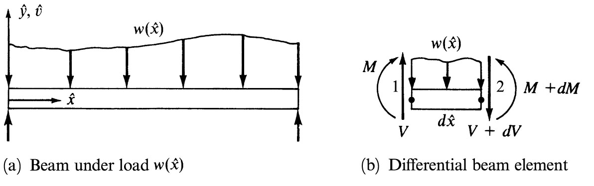
"# Euler-Bernoulli Beam Element\n",
"\n",
"In Euler-Bernoulli beam theory, it is assumed that plane sections remain\n",
"plane. In this theory, the transverse deflection $u$ of the beam is governed\n",
"by\n",
"\n",
"$$\n",
"\\frac{d^2}{dx^2}\\left( a\\frac{d^2u}{dx^2}\\right) +q(x)=0\n",
"$$\n",
"\n",
"In the figure below, a typical beam, with sign conventions is shown\n",
"\n",
"
\n",
"\n",
"This lecture by Tim Fuller is licensed under the\n",
"Creative Commons Attribution 4.0 International License. All code examples are also licensed under the [MIT license](http://opensource.org/licenses/MIT)."
]
},
{
"cell_type": "markdown",
"metadata": {},
"source": [
"# Topics\n",
"- [Introduction](#intro)\n",
"- [Beam Element](#beam-el)\n",
" - [$Discretization of the Domain](#disc)\n",
" - [Derivation of Element Equations](#derive)"
]
},
{
"cell_type": "markdown",
"metadata": {},
"source": [
"# Introduction\n",
"\n",
"In the last two lectures we discussed the finite element formulation of one dimensional second order BVPs and we completed examples in thermal, fluid, and solid mechanics. Today we discuss the finite element formulation of the one dimensional fourth order BVP associated with the Euler-Bernoulli beam theory. The formulation of the finite element equations is obtained by following the same steps as in the second order BVP finite element formulation."
]
},
{
"cell_type": "markdown",
"metadata": {},
"source": [
"# Euler-Bernoulli Beam Element\n",
"\n",
"In Euler-Bernoulli beam theory, it is assumed that plane sections remain\n",
"plane. In this theory, the transverse deflection $u$ of the beam is governed\n",
"by\n",
"\n",
"$$\n",
"\\frac{d^2}{dx^2}\\left( a\\frac{d^2u}{dx^2}\\right) +q(x)=0\n",
"$$\n",
"\n",
"In the figure below, a typical beam, with sign conventions is shown\n",
"\n",
" \n",
"\n",
"Here $a=a(x)$ and $q=q(x)$ are the given problem data and $u$ is the dependent\n",
"variable. The function $a=EI$ is the flexural rigidity of the beam, $q$ is the\n",
"transversely distributed load, and $u$ is the transverse deflection. In\n",
"addition to satisfying the beam bending equation, $u$ must also satisfy the\n",
"boundary conditions. Since beam bending is governed by a fourth order DE, four\n",
"boundary conditions are required to solve it. As in the second order DEs we\n",
"previously solved, the appropriate boundary conditions arise from the weak\n",
"form of the governing equation. We now develop the finite element equations\n",
"for a beam.\n",
"\n",
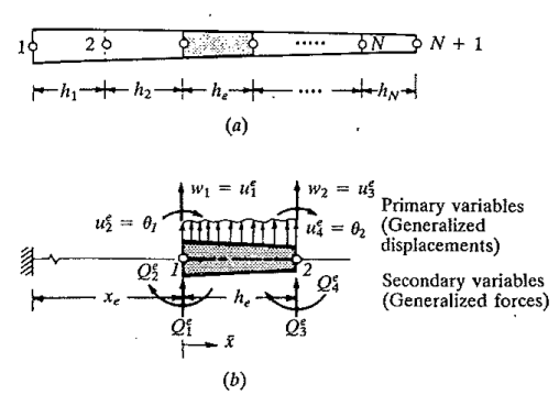
"## Discretization of the Domain\n",
"\n",
"The domain (length) of the beam is divided into $N-1$ line elements, each having at least two end nodes, as shown below. Note that the element geometry is the same as with the bar element, however, the number and form of the primary and secondary unknowns at each node is different and are dictated by the variational (weak) formulation of the beam equation.\n",
"\n",
"
\n",
"\n",
"Here $a=a(x)$ and $q=q(x)$ are the given problem data and $u$ is the dependent\n",
"variable. The function $a=EI$ is the flexural rigidity of the beam, $q$ is the\n",
"transversely distributed load, and $u$ is the transverse deflection. In\n",
"addition to satisfying the beam bending equation, $u$ must also satisfy the\n",
"boundary conditions. Since beam bending is governed by a fourth order DE, four\n",
"boundary conditions are required to solve it. As in the second order DEs we\n",
"previously solved, the appropriate boundary conditions arise from the weak\n",
"form of the governing equation. We now develop the finite element equations\n",
"for a beam.\n",
"\n",
"## Discretization of the Domain\n",
"\n",
"The domain (length) of the beam is divided into $N-1$ line elements, each having at least two end nodes, as shown below. Note that the element geometry is the same as with the bar element, however, the number and form of the primary and secondary unknowns at each node is different and are dictated by the variational (weak) formulation of the beam equation.\n",
"\n",
" \n",
"\n",
"## Derivation of Element Equations\n",
"\n",
"We now isolate a typical element $\\Omega^{(e)}=(x_A,x_B)$ and construct the\n",
"weak form of the beam bending equation over that element. Recall that the weak\n",
"form provides the primary and secondary variables of the problem. We will then\n",
"choose approximation for the primary variable and derive the element\n",
"equations."
]
},
{
"cell_type": "markdown",
"metadata": {},
"source": [
"### The Weak Form\n",
"\n",
"We derive the weak form in the same way as with the second order BVP, namely,\n",
"we multiply the governing equation by a weight function $w(x)$, integrate by\n",
"parts to reduce the continuity requirements on $u$, and evaluate the resulting\n",
"boundary conditions.\n",
"\n",
"$$\n",
"\\begin{gather}\n",
"\\int_{x_A}^{x_B}\\left(\\frac{d^2}{dx^2}\\left(a\\frac{d^2u}{dx^2} \\right) + q \\right) w dx = 0 \\\\\n",
"\\int_{x_A}^{x_B}\\left( -\\frac{dw}{dx}\\frac{d}{dx}\\left( a \\frac{d^2u}{dx^2}\\right) + wq \\right) dx + \\left[ w\\frac{d}{dx}\\left( a\\frac{d^2u}{dx^2} \\right) \\right]_{x_A}^{x_B} =0 \\\\\n",
"\\int_{x_A}^{x_B}\\left( a\\frac{d^2w}{dx^2}\\frac{d^2u}{dx^2}+wq\\right) dx + \\left[ w\\frac{d}{dx}\\left( a\\frac{d^2u}{dx^2} \\right)-\\frac{dw}{dx}a\\frac{d^2u}{dx^2} \\right]_{x_A}^{x_B} =0\n",
"\\end{gather}\n",
"$$\n",
"\n",
"Note that, because of the two integrations by parts, $u,w\\in C^1$. We have\n",
"reduced the continuity requirements on $u$ from $C^3$ to $C^1$. Also, because\n",
"of the integration by parts, there are now two boundary terms to be evaluated\n",
"at $x=x_A$ and $x=x_B$. Let's look closely at the two boundary conditions:\n",
"\n",
"$$\n",
"\\left[ w\\frac{d}{dx}\\left( a\\frac{d^2u}{dx^2} \\right)-\\frac{dw}{dx}a\\frac{d^2u}{dx^2} \\right]_{x_A}^{x_B}\n",
"$$\n",
"\n",
"From the boundary conditions, it follows that the specification of $u$ and\n",
"$du/dx$ at the endpoints of the elements constitute the essential boundary\n",
"conditions and the specification of\n",
"\n",
"$$\n",
"\\frac{d}{dx}\\left( a\\frac{d^2u}{dx^2} \\right)=V \\quad (\\text{shear force})\n",
"$$\n",
"\n",
"and\n",
"\n",
"$$\n",
"a\\frac{d^2u}{dx^2} =M \\quad (\\text{bending moment})\n",
"$$\n",
"\n",
"at the endpoints constitute the natural boundary conditions. Thus, their are\n",
"two essential and two natural boundary conditions. Therefore, we identify $u$\n",
"and $du/dx$ as the primary variables at each node. The natural boundary\n",
"conditions always remain in the weak form and end up as the source vector of\n",
"the matrix equations. To simplify notation, we introduce the the notation\n",
"$\\phi=du/dx$ and\n",
"\n",
"$$\\begin{gather}\n",
"Q_1^{(e)}=V_1^{(e)}=\\left[ \\frac{d}{dx}\\left( a\\frac{d^2u}{dx^2} \\right) \\right]\\Bigg|_{{x_A}}, \\quad Q_2^{(e)}=M_1^{(e)}=\\left( a\\frac{d^2u}{dx^2} \\right) \\Bigg|_{x_A}\\\\\n",
"Q_3^{(e)}=V_2^{(e)}=-\\left[ \\frac{d}{dx}\\left( a\\frac{d^2u}{dx^2} \\right) \\right]\\Bigg|_{x_B}, \\quad Q_4^{(e)}=M_2^{(e)}=-\\left( a\\frac{d^2u}{dx^2} \\right) \\Bigg|_{x_B}\\\\\n",
"\\end{gather}\n",
"$$\n",
"\n",
"where $Q_1^{(e)}$ and $Q_3^{(e)}$ denote the shear forces, and $Q_2^{(e)}$ and\n",
"$Q_4^{(e)}$ denote the bending moments shown in \\rfig{bd0}. Since the set\n",
"$Q_i^{(e)}$ contain both point and ''bending'' forces, we will call the set\n",
"\n",
"$$\n",
"\\begin{Bmatrix} Q_1^{(e)} \\\\ Q_2^{(e)}\\\\ Q_3^{(e)}\\\\ Q_4^{(e)} \\end{Bmatrix}\n",
"$$\n",
"\n",
"the *generalized forces*. We call the corresponding set of displacements and\n",
"rotations the *generalized displacements*:\n",
"\n",
"$$\n",
"\\begin{Bmatrix} u(x_A) \\\\ u'(x_A) \\\\ u(x_B) \\\\ u'(x_B) \\end{Bmatrix} =\n",
"\\begin{Bmatrix} u_1^{(e)} \\\\ u_2^{(e)} \\\\ u_3^{(e)} \\\\ u_4^{(e)}\\end{Bmatrix} =\n",
"\\begin{Bmatrix} u_1 \\\\ \\phi_1 \\\\ u_2 \\\\ \\phi_2\\end{Bmatrix}\n",
"$$\n",
"\n",
"With this notation, we can now write\n",
"\n",
"$$\n",
"\\int_{x_A}^{x_B}\\left( b\\frac{d^2w}{dx^2}\\frac{d^2u}{dx^2}+qw\\right) dx + \\left[ wV-\\frac{dw}{dx}M\\right]\\Bigg|_{x_A}^{x_B} =0\n",
"$$"
]
},
{
"cell_type": "markdown",
"metadata": {},
"source": [
"### Interpolation Functions\n",
"The weak form requires that the interpolation functions of an element be continuous with nonzero derivatives up to order two. The approximation of the primary variables over a finite element should be such that it satisfies the essential boundary conditions of the element:\n",
"\n",
"$$\n",
"u(x_A)=u_1, \\quad u(x_B)=u_2, \\quad \\phi(x_A)=\\phi_1, \\quad \\phi(x_B)=\\phi_2\n",
"$$\n",
"\n",
"Since there is a total of four conditions in an element (two per node), a four parameter polynomial must be selected for $u$:\n",
"\n",
"$$\n",
"u(x)=u_0 + u_1x + u_2x^2 + u_3x^3\n",
"$$\n",
"\n",
"We now express the $c_i$ in terms of the general displacements and require that\n",
"\n",
"$$\n",
"u(x_A)=u_1^{(e)}=u_0 + u_1x_A+u_2x_A^2+u_3x_A^3\\\\\n",
"\\phi(x_A)= u_2^{(e)}=u_1 + 2u_2x_A+3u_3x_A^2\\\\\n",
"u(x_B)=u_3^{(e)}=u_0 + u_1x_B+u_2x_B^2+u_3x_B^3\\\\\n",
"\\phi(x_B)= u_4^{(e)}=+u_1 + 2u_2x_B+3u_3x_B^2\n",
"$$\n",
"\n",
"or\n",
"\n",
"$$\n",
"\\begin{Bmatrix} u_1^{(e)} \\\\ u_2^{(e)} \\\\ u_3^{(e)} \\\\ u_4^{(e)} \\end{Bmatrix} =\n",
"\\begin{bmatrix} 1 & x_A & x_A^2 & x_A^3 \\\\ 0 & 1 & 2x_A & 3x_A^2 \\\\ 1 & x_B & x_B^2 & x_B^3 \\\\ 0 & 1 & 2x_B & 3x_B^2\\end{bmatrix}\n",
"\\begin{Bmatrix} u_0 \\\\ u_1 \\\\ u_2 \\\\ u_3 \\end{Bmatrix}\n",
"$$\n",
"\n",
"Inverting this expression to express the $u_i$ in terms of the $u_i^{(e)}$ and substituting the result gives\n",
"\n",
"$$\n",
"u^{(e)}(x)=u_1^{(e)}N_1^{(e)}+u_2^{(e)}N_2^{(e)}+u_3^{(e)}N_3^{(e)}+u_4^{(e)}N_4^{(e)}=\\sum_{j=1}^4u_j^{(e)}N_j^{(e)}\n",
"$$\n",
"\n",
"where\n",
"\n",
"$$\n",
"N_1^{(e)}=1-3\\left(\\frac{x-x_A}{h_e}\\right)^2+2\\left(\\frac{x-x_A}{h_e}\\right)^3, \\ \\ \\ N_2^{(e)}=\\left( x-x_A\\right)\\left( \\frac{x-x_A}{h_e}-1\\right)^2\\\\\n",
"N_3^{(e)}=3\\left(\\frac{x-x_A}{h_e}\\right)^2-2\\left(\\frac{x-x_A}{h_e}\\right)^3, \\ \\ \\ N_4^{(e)}=\\left( x-x_A\\right)\\left(\\left(\\frac{x-x_A}{h_e}\\right)^2-\\frac{x-x_A}{h_e}\\right)\n",
"$$\n",
"\n",
"Note that the cubic interpolation functions were derived by interpolating $u$\n",
"and its derivatives at the nodes. Interpolation polynomials derived in this\n",
"way are known as Hermite interpolation functions.\n",
"\n",
"The shape functions $N_i^{(e)}$ can be expressed in terms of the local coordinates $\\hat{x}$:\n",
"\n",
"$$\n",
"N_1^{(e)}=1-3\\left(\\frac{\\hat{x}}{h_e}\\right)^2+2\\left(\\frac{\\hat{x}}{h_e}\\right)^3, \\ \\ \\ N_2^{(e)}=\\hat{x}\\left( \\frac{\\hat{x}}{h_e}-1\\right)^2\\\\\n",
"N_3^{(e)}=3\\left(\\frac{\\hat{x}}{h_e}\\right)^2-2\\left(\\frac{\\hat{x}}{h_e}\\right)^3, \\ \\ \\ N_4^{(e)}=\\hat{x}\\left(\\left(\\frac{\\hat{x}}{h_e}\\right)^2-\\frac{\\hat{x}}{h_e}\\right)\n",
"$$\n",
"\n",
"The Hermite cubic interpolation functions satisfy the following interpolation properties ($i,j=1,2$)\n",
"\n",
"$$\n",
"N_{2i-1}^{(e)}(\\hat{x}_j)=\\delta_{ij}, \\ \\ \\ \\ N_{2i}^{(e)}(\\hat{x}_j)=0, \\ \\ \\ \\ \\sum_{i=1}^2N_{2i-1}^{(e)}=1\\\\\n",
"\\frac{dN_{2i-1}^{e}}{dx}\\Bigg|_{\\hat{x}_j}=0, \\ \\ \\ \\ \\frac{dN_{2i}^{(e)}}{dx}\\Bigg|_{\\hat{x}_j}=\\delta_{ij}\n",
"$$\n",
"\n",
"where $\\hat{x}_1=0$ and $\\hat{x}_2=h_e$ are the local coordinates of nodes 1 and 2 of the element $\\Omega^{(e)}=(x_A,x_B)$.\\\\"
]
},
{
"cell_type": "markdown",
"metadata": {},
"source": [
"### Finite Element Model\n",
"\n",
"We now substitute\n",
"$$\n",
"u^{(e)}(x)=\\sum_{j=1}^4 u_j^{(e)}N_j^{(e)}\n",
"$$\n",
"and\n",
"$$\n",
"w=\\sum_{i=1}^4 w_i^{(e)}N_i^{(e)}\n",
"$$\n",
"\n",
"Substituting and simplifying gives\n",
"\n",
"$$\n",
"\\sum_{j=1}^4\\left(\\int_{x_A}^{x_B}a\\frac{d^2N_i^{(e)}}{dx^2}\\frac{d^2N_{j}^{(e)}}{dx^2}dx\\right) u_j^{(e)} + \\int_{x_A}^{x_B}N_i^{(e)}qdx-Q_i^{(e)}=0\n",
"$$\n",
"\n",
"or\n",
"\n",
"$$\n",
"\\sum_{j=1}^4k_{ij}^{(e)}u_j^{(e)}+F_i^{(e)}=0\n",
"$$\n",
"where\n",
"\n",
"$$\n",
"k_{ij}^{(e)}=\\int_{x_A}^{x_B}a\\frac{d^2N_i^{(e)}}{dx^2}\\frac{d^2N_j^{(e)}}{dx^2}dx, \\ \\ \\ \\ F_i^{(e)} = \\int_{x_A}^{x_B}N_i^{(e)}qdx-Q_i^{(e)}\n",
"$$\n",
"\n",
"In matrix notation this can be written\n",
"\n",
"$$\n",
"\\begin{bmatrix} \n",
"k_{11}^{(e)} & k_{12}^{(e)} & k_{13}^3 & k_{14}^{(e)} \\\\ \n",
"k_{21}^{(e)} & k_{22}^{(e)} & k_{23}^3 & k_{24}^{(e)} \\\\ \n",
"k_{31}^{(e)} & k_{32}^{(e)} & k_{33}^3 & k_{34}^{(e)} \\\\ \n",
"k_{41}^{(e)} & k_{42}^{(e)} & k_{43}^3 & k_{44}^{(e)} \n",
"\\end{bmatrix} \n",
"\\begin{Bmatrix} \n",
"u_1^{(e)} \\\\ u_2^{(e)} \\\\ u_3^{(e)} \\\\ u_4^{(e)} \n",
"\\end{Bmatrix} = \n",
"-\\begin{Bmatrix} q_1^{(e)} \\\\ q_2^{(e)} \\\\ q_3^{(e)} \\\\ q_4^{(e)} \\end{Bmatrix} + \\begin{Bmatrix} Q_1^{(e)} \\\\ Q_2^{(e)} \\\\ Q_3^{(e)} \\\\ Q_4^{(e)} \\end{Bmatrix}\n",
"$$\n",
"\n",
"For the case in which $a=EI$ and $w$ are constant over an element, the coefficients of each element equation are found as with the bar element:\n",
"\n",
"$$\n",
"k_{11}^{(e)}=EI\\int_0^{h_e}\\frac{d^2N_1^{(e)}}{d\\hat{x}^2}\\frac{d^2N_1^{(e)}}{d\\hat{x}^2} \\ d\\hat x=EI\\int_0^{h_e}\\left(-\\frac{6}{h_e^{2}}+12\\,{\\frac {\\hat x}{h_e^{3}}}\\right)^2 \\ d\\hat x=\\frac{12EI}{h_e^3}\n",
"$$\n",
"\n",
"$$\n",
"F_1^{(e)}=q\\int_0^{h_e}N_1^{(e)} \\ d\\hat x - Q_1^{(e)} =q\\int_0^{h_e}\\left(-\\frac{6}{h_e^{2}}+12\\,{\\frac {\\hat x}{h_e^{3}}}\\right) d\\hat x - V_1^{(e)} = \\frac{qh_e}{2} - V_1^{(e)}\n",
"$$\n",
"\n",
"All other coefficients can be found in a similar manner and combine to give the beam equations for a single two node element:\n",
"\n",
"$$\n",
"\\frac{2EI}{h_e^3}\\begin{bmatrix}\n",
"6 & 3h_e & -6 & 3h_e \\\\\n",
"3h_e & 2h_e^2 & -3h_e & h_e^2 \\\\\n",
"-6 & -3h_e & 6 & -3h_e \\\\\n",
"3h_e & h_e^2 & -3h_e & 2h_e^2 \\end{bmatrix}\\begin{Bmatrix} u_1^{(e)} \\\\ \\phi_1^{(e)} \\\\ u_2^{(e)} \\\\ \\phi_2^{(e)} \\end{Bmatrix}=-\\frac{wh_e}{12}\\begin{Bmatrix}6\\\\h_e\\\\6\\\\-h_e\\end{Bmatrix}+\\begin{Bmatrix}V_1^{(e)}\\\\M_1^{(e)}\\\\ V_2^{(e)}\\\\M_2^{(e)}\\end{Bmatrix}\n",
"$$"
]
},
{
"cell_type": "markdown",
"metadata": {},
"source": [
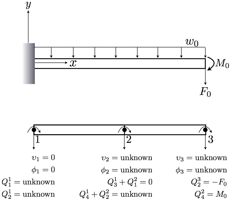
"### Assembly of Global Equations\n",
"\n",
"We assemble the global equations in the same way as the bar element equation, except we take into account the increased degrees of freedom at element nodes. The assembly of the global equations is based on:\n",
"\n",
"\n",
"- Interelement continuity of primary variables (deflection and slope)\n",
"- Interelement equilibrium of the secondary variables (shear force and bending moment) at the nodes of common elements\n",
"\n",
"We demonstrate the assembly of the global equations by examining the following two element model\n",
"\n",
"
\n",
"\n",
"## Derivation of Element Equations\n",
"\n",
"We now isolate a typical element $\\Omega^{(e)}=(x_A,x_B)$ and construct the\n",
"weak form of the beam bending equation over that element. Recall that the weak\n",
"form provides the primary and secondary variables of the problem. We will then\n",
"choose approximation for the primary variable and derive the element\n",
"equations."
]
},
{
"cell_type": "markdown",
"metadata": {},
"source": [
"### The Weak Form\n",
"\n",
"We derive the weak form in the same way as with the second order BVP, namely,\n",
"we multiply the governing equation by a weight function $w(x)$, integrate by\n",
"parts to reduce the continuity requirements on $u$, and evaluate the resulting\n",
"boundary conditions.\n",
"\n",
"$$\n",
"\\begin{gather}\n",
"\\int_{x_A}^{x_B}\\left(\\frac{d^2}{dx^2}\\left(a\\frac{d^2u}{dx^2} \\right) + q \\right) w dx = 0 \\\\\n",
"\\int_{x_A}^{x_B}\\left( -\\frac{dw}{dx}\\frac{d}{dx}\\left( a \\frac{d^2u}{dx^2}\\right) + wq \\right) dx + \\left[ w\\frac{d}{dx}\\left( a\\frac{d^2u}{dx^2} \\right) \\right]_{x_A}^{x_B} =0 \\\\\n",
"\\int_{x_A}^{x_B}\\left( a\\frac{d^2w}{dx^2}\\frac{d^2u}{dx^2}+wq\\right) dx + \\left[ w\\frac{d}{dx}\\left( a\\frac{d^2u}{dx^2} \\right)-\\frac{dw}{dx}a\\frac{d^2u}{dx^2} \\right]_{x_A}^{x_B} =0\n",
"\\end{gather}\n",
"$$\n",
"\n",
"Note that, because of the two integrations by parts, $u,w\\in C^1$. We have\n",
"reduced the continuity requirements on $u$ from $C^3$ to $C^1$. Also, because\n",
"of the integration by parts, there are now two boundary terms to be evaluated\n",
"at $x=x_A$ and $x=x_B$. Let's look closely at the two boundary conditions:\n",
"\n",
"$$\n",
"\\left[ w\\frac{d}{dx}\\left( a\\frac{d^2u}{dx^2} \\right)-\\frac{dw}{dx}a\\frac{d^2u}{dx^2} \\right]_{x_A}^{x_B}\n",
"$$\n",
"\n",
"From the boundary conditions, it follows that the specification of $u$ and\n",
"$du/dx$ at the endpoints of the elements constitute the essential boundary\n",
"conditions and the specification of\n",
"\n",
"$$\n",
"\\frac{d}{dx}\\left( a\\frac{d^2u}{dx^2} \\right)=V \\quad (\\text{shear force})\n",
"$$\n",
"\n",
"and\n",
"\n",
"$$\n",
"a\\frac{d^2u}{dx^2} =M \\quad (\\text{bending moment})\n",
"$$\n",
"\n",
"at the endpoints constitute the natural boundary conditions. Thus, their are\n",
"two essential and two natural boundary conditions. Therefore, we identify $u$\n",
"and $du/dx$ as the primary variables at each node. The natural boundary\n",
"conditions always remain in the weak form and end up as the source vector of\n",
"the matrix equations. To simplify notation, we introduce the the notation\n",
"$\\phi=du/dx$ and\n",
"\n",
"$$\\begin{gather}\n",
"Q_1^{(e)}=V_1^{(e)}=\\left[ \\frac{d}{dx}\\left( a\\frac{d^2u}{dx^2} \\right) \\right]\\Bigg|_{{x_A}}, \\quad Q_2^{(e)}=M_1^{(e)}=\\left( a\\frac{d^2u}{dx^2} \\right) \\Bigg|_{x_A}\\\\\n",
"Q_3^{(e)}=V_2^{(e)}=-\\left[ \\frac{d}{dx}\\left( a\\frac{d^2u}{dx^2} \\right) \\right]\\Bigg|_{x_B}, \\quad Q_4^{(e)}=M_2^{(e)}=-\\left( a\\frac{d^2u}{dx^2} \\right) \\Bigg|_{x_B}\\\\\n",
"\\end{gather}\n",
"$$\n",
"\n",
"where $Q_1^{(e)}$ and $Q_3^{(e)}$ denote the shear forces, and $Q_2^{(e)}$ and\n",
"$Q_4^{(e)}$ denote the bending moments shown in \\rfig{bd0}. Since the set\n",
"$Q_i^{(e)}$ contain both point and ''bending'' forces, we will call the set\n",
"\n",
"$$\n",
"\\begin{Bmatrix} Q_1^{(e)} \\\\ Q_2^{(e)}\\\\ Q_3^{(e)}\\\\ Q_4^{(e)} \\end{Bmatrix}\n",
"$$\n",
"\n",
"the *generalized forces*. We call the corresponding set of displacements and\n",
"rotations the *generalized displacements*:\n",
"\n",
"$$\n",
"\\begin{Bmatrix} u(x_A) \\\\ u'(x_A) \\\\ u(x_B) \\\\ u'(x_B) \\end{Bmatrix} =\n",
"\\begin{Bmatrix} u_1^{(e)} \\\\ u_2^{(e)} \\\\ u_3^{(e)} \\\\ u_4^{(e)}\\end{Bmatrix} =\n",
"\\begin{Bmatrix} u_1 \\\\ \\phi_1 \\\\ u_2 \\\\ \\phi_2\\end{Bmatrix}\n",
"$$\n",
"\n",
"With this notation, we can now write\n",
"\n",
"$$\n",
"\\int_{x_A}^{x_B}\\left( b\\frac{d^2w}{dx^2}\\frac{d^2u}{dx^2}+qw\\right) dx + \\left[ wV-\\frac{dw}{dx}M\\right]\\Bigg|_{x_A}^{x_B} =0\n",
"$$"
]
},
{
"cell_type": "markdown",
"metadata": {},
"source": [
"### Interpolation Functions\n",
"The weak form requires that the interpolation functions of an element be continuous with nonzero derivatives up to order two. The approximation of the primary variables over a finite element should be such that it satisfies the essential boundary conditions of the element:\n",
"\n",
"$$\n",
"u(x_A)=u_1, \\quad u(x_B)=u_2, \\quad \\phi(x_A)=\\phi_1, \\quad \\phi(x_B)=\\phi_2\n",
"$$\n",
"\n",
"Since there is a total of four conditions in an element (two per node), a four parameter polynomial must be selected for $u$:\n",
"\n",
"$$\n",
"u(x)=u_0 + u_1x + u_2x^2 + u_3x^3\n",
"$$\n",
"\n",
"We now express the $c_i$ in terms of the general displacements and require that\n",
"\n",
"$$\n",
"u(x_A)=u_1^{(e)}=u_0 + u_1x_A+u_2x_A^2+u_3x_A^3\\\\\n",
"\\phi(x_A)= u_2^{(e)}=u_1 + 2u_2x_A+3u_3x_A^2\\\\\n",
"u(x_B)=u_3^{(e)}=u_0 + u_1x_B+u_2x_B^2+u_3x_B^3\\\\\n",
"\\phi(x_B)= u_4^{(e)}=+u_1 + 2u_2x_B+3u_3x_B^2\n",
"$$\n",
"\n",
"or\n",
"\n",
"$$\n",
"\\begin{Bmatrix} u_1^{(e)} \\\\ u_2^{(e)} \\\\ u_3^{(e)} \\\\ u_4^{(e)} \\end{Bmatrix} =\n",
"\\begin{bmatrix} 1 & x_A & x_A^2 & x_A^3 \\\\ 0 & 1 & 2x_A & 3x_A^2 \\\\ 1 & x_B & x_B^2 & x_B^3 \\\\ 0 & 1 & 2x_B & 3x_B^2\\end{bmatrix}\n",
"\\begin{Bmatrix} u_0 \\\\ u_1 \\\\ u_2 \\\\ u_3 \\end{Bmatrix}\n",
"$$\n",
"\n",
"Inverting this expression to express the $u_i$ in terms of the $u_i^{(e)}$ and substituting the result gives\n",
"\n",
"$$\n",
"u^{(e)}(x)=u_1^{(e)}N_1^{(e)}+u_2^{(e)}N_2^{(e)}+u_3^{(e)}N_3^{(e)}+u_4^{(e)}N_4^{(e)}=\\sum_{j=1}^4u_j^{(e)}N_j^{(e)}\n",
"$$\n",
"\n",
"where\n",
"\n",
"$$\n",
"N_1^{(e)}=1-3\\left(\\frac{x-x_A}{h_e}\\right)^2+2\\left(\\frac{x-x_A}{h_e}\\right)^3, \\ \\ \\ N_2^{(e)}=\\left( x-x_A\\right)\\left( \\frac{x-x_A}{h_e}-1\\right)^2\\\\\n",
"N_3^{(e)}=3\\left(\\frac{x-x_A}{h_e}\\right)^2-2\\left(\\frac{x-x_A}{h_e}\\right)^3, \\ \\ \\ N_4^{(e)}=\\left( x-x_A\\right)\\left(\\left(\\frac{x-x_A}{h_e}\\right)^2-\\frac{x-x_A}{h_e}\\right)\n",
"$$\n",
"\n",
"Note that the cubic interpolation functions were derived by interpolating $u$\n",
"and its derivatives at the nodes. Interpolation polynomials derived in this\n",
"way are known as Hermite interpolation functions.\n",
"\n",
"The shape functions $N_i^{(e)}$ can be expressed in terms of the local coordinates $\\hat{x}$:\n",
"\n",
"$$\n",
"N_1^{(e)}=1-3\\left(\\frac{\\hat{x}}{h_e}\\right)^2+2\\left(\\frac{\\hat{x}}{h_e}\\right)^3, \\ \\ \\ N_2^{(e)}=\\hat{x}\\left( \\frac{\\hat{x}}{h_e}-1\\right)^2\\\\\n",
"N_3^{(e)}=3\\left(\\frac{\\hat{x}}{h_e}\\right)^2-2\\left(\\frac{\\hat{x}}{h_e}\\right)^3, \\ \\ \\ N_4^{(e)}=\\hat{x}\\left(\\left(\\frac{\\hat{x}}{h_e}\\right)^2-\\frac{\\hat{x}}{h_e}\\right)\n",
"$$\n",
"\n",
"The Hermite cubic interpolation functions satisfy the following interpolation properties ($i,j=1,2$)\n",
"\n",
"$$\n",
"N_{2i-1}^{(e)}(\\hat{x}_j)=\\delta_{ij}, \\ \\ \\ \\ N_{2i}^{(e)}(\\hat{x}_j)=0, \\ \\ \\ \\ \\sum_{i=1}^2N_{2i-1}^{(e)}=1\\\\\n",
"\\frac{dN_{2i-1}^{e}}{dx}\\Bigg|_{\\hat{x}_j}=0, \\ \\ \\ \\ \\frac{dN_{2i}^{(e)}}{dx}\\Bigg|_{\\hat{x}_j}=\\delta_{ij}\n",
"$$\n",
"\n",
"where $\\hat{x}_1=0$ and $\\hat{x}_2=h_e$ are the local coordinates of nodes 1 and 2 of the element $\\Omega^{(e)}=(x_A,x_B)$.\\\\"
]
},
{
"cell_type": "markdown",
"metadata": {},
"source": [
"### Finite Element Model\n",
"\n",
"We now substitute\n",
"$$\n",
"u^{(e)}(x)=\\sum_{j=1}^4 u_j^{(e)}N_j^{(e)}\n",
"$$\n",
"and\n",
"$$\n",
"w=\\sum_{i=1}^4 w_i^{(e)}N_i^{(e)}\n",
"$$\n",
"\n",
"Substituting and simplifying gives\n",
"\n",
"$$\n",
"\\sum_{j=1}^4\\left(\\int_{x_A}^{x_B}a\\frac{d^2N_i^{(e)}}{dx^2}\\frac{d^2N_{j}^{(e)}}{dx^2}dx\\right) u_j^{(e)} + \\int_{x_A}^{x_B}N_i^{(e)}qdx-Q_i^{(e)}=0\n",
"$$\n",
"\n",
"or\n",
"\n",
"$$\n",
"\\sum_{j=1}^4k_{ij}^{(e)}u_j^{(e)}+F_i^{(e)}=0\n",
"$$\n",
"where\n",
"\n",
"$$\n",
"k_{ij}^{(e)}=\\int_{x_A}^{x_B}a\\frac{d^2N_i^{(e)}}{dx^2}\\frac{d^2N_j^{(e)}}{dx^2}dx, \\ \\ \\ \\ F_i^{(e)} = \\int_{x_A}^{x_B}N_i^{(e)}qdx-Q_i^{(e)}\n",
"$$\n",
"\n",
"In matrix notation this can be written\n",
"\n",
"$$\n",
"\\begin{bmatrix} \n",
"k_{11}^{(e)} & k_{12}^{(e)} & k_{13}^3 & k_{14}^{(e)} \\\\ \n",
"k_{21}^{(e)} & k_{22}^{(e)} & k_{23}^3 & k_{24}^{(e)} \\\\ \n",
"k_{31}^{(e)} & k_{32}^{(e)} & k_{33}^3 & k_{34}^{(e)} \\\\ \n",
"k_{41}^{(e)} & k_{42}^{(e)} & k_{43}^3 & k_{44}^{(e)} \n",
"\\end{bmatrix} \n",
"\\begin{Bmatrix} \n",
"u_1^{(e)} \\\\ u_2^{(e)} \\\\ u_3^{(e)} \\\\ u_4^{(e)} \n",
"\\end{Bmatrix} = \n",
"-\\begin{Bmatrix} q_1^{(e)} \\\\ q_2^{(e)} \\\\ q_3^{(e)} \\\\ q_4^{(e)} \\end{Bmatrix} + \\begin{Bmatrix} Q_1^{(e)} \\\\ Q_2^{(e)} \\\\ Q_3^{(e)} \\\\ Q_4^{(e)} \\end{Bmatrix}\n",
"$$\n",
"\n",
"For the case in which $a=EI$ and $w$ are constant over an element, the coefficients of each element equation are found as with the bar element:\n",
"\n",
"$$\n",
"k_{11}^{(e)}=EI\\int_0^{h_e}\\frac{d^2N_1^{(e)}}{d\\hat{x}^2}\\frac{d^2N_1^{(e)}}{d\\hat{x}^2} \\ d\\hat x=EI\\int_0^{h_e}\\left(-\\frac{6}{h_e^{2}}+12\\,{\\frac {\\hat x}{h_e^{3}}}\\right)^2 \\ d\\hat x=\\frac{12EI}{h_e^3}\n",
"$$\n",
"\n",
"$$\n",
"F_1^{(e)}=q\\int_0^{h_e}N_1^{(e)} \\ d\\hat x - Q_1^{(e)} =q\\int_0^{h_e}\\left(-\\frac{6}{h_e^{2}}+12\\,{\\frac {\\hat x}{h_e^{3}}}\\right) d\\hat x - V_1^{(e)} = \\frac{qh_e}{2} - V_1^{(e)}\n",
"$$\n",
"\n",
"All other coefficients can be found in a similar manner and combine to give the beam equations for a single two node element:\n",
"\n",
"$$\n",
"\\frac{2EI}{h_e^3}\\begin{bmatrix}\n",
"6 & 3h_e & -6 & 3h_e \\\\\n",
"3h_e & 2h_e^2 & -3h_e & h_e^2 \\\\\n",
"-6 & -3h_e & 6 & -3h_e \\\\\n",
"3h_e & h_e^2 & -3h_e & 2h_e^2 \\end{bmatrix}\\begin{Bmatrix} u_1^{(e)} \\\\ \\phi_1^{(e)} \\\\ u_2^{(e)} \\\\ \\phi_2^{(e)} \\end{Bmatrix}=-\\frac{wh_e}{12}\\begin{Bmatrix}6\\\\h_e\\\\6\\\\-h_e\\end{Bmatrix}+\\begin{Bmatrix}V_1^{(e)}\\\\M_1^{(e)}\\\\ V_2^{(e)}\\\\M_2^{(e)}\\end{Bmatrix}\n",
"$$"
]
},
{
"cell_type": "markdown",
"metadata": {},
"source": [
"### Assembly of Global Equations\n",
"\n",
"We assemble the global equations in the same way as the bar element equation, except we take into account the increased degrees of freedom at element nodes. The assembly of the global equations is based on:\n",
"\n",
"\n",
"- Interelement continuity of primary variables (deflection and slope)\n",
"- Interelement equilibrium of the secondary variables (shear force and bending moment) at the nodes of common elements\n",
"\n",
"We demonstrate the assembly of the global equations by examining the following two element model\n",
"\n",
" \n",
"\n",
"The continuity of the primary variables implies the following relation between the element degrees of freedom $u_i^{(e)}$ and the global degrees of freedom $u_i$ and $\\phi_i$:\n",
"\n",
"$$ \\begin{matrix}\n",
"u_1^1=u_1 & u_2^1=\\phi_1 & u_3^1=u_1^2=u_2 \\\\\n",
"u_4^1=u_2^2=\\phi_2 & u_3^2=u_3 & u_4^2=\\phi_3 \\end{matrix}\n",
"$$\n",
"\n",
"The equilibrium of the forces and moments at the connecting node requires that\n",
"$$\n",
"Q_3^1+Q_1^2={\\rm applied \\ external \\ point \\ force}=0\n",
"$$\n",
"\n",
"$$\n",
"Q_4^1+Q_2^2={\\rm applied \\ external \\ bending \\ moment}=0\n",
"$$\n",
"\n",
"If no external applied forces are given, the sum should be equated to zero. In equating the sums to the applied generalized forces (i.e. the force or moment) the sign convention for the element force degrees of freedom should be followed. Forces are taken positive acting upwards and moments positive taken clockwise.\\\\\n",
"\n",
"We now expand each element equation to the size of the global equation and combine them to form the global set of equations:\n",
"\n",
"### Element 1\n",
"$$\n",
"\\begin{bmatrix} k_{11}^1 & k_{12}^1 & k_{13}^1 & k_{14}^1 & 0 & 0\\\\\n",
" \t\t k_{21}^1 & k_{22}^1 & k_{23}^1 & k_{24}^1 & 0 & 0\\\\\n",
"\t\t\tk_{31}^1 & k_{32}^1 & k_{33}^1 & k_{34}^1 & 0 & 0\\\\\n",
"\t\t\tk_{41}^1 & k_{42}^1 & k_{43}^1 & k_{44}^1 & 0 & 0\\\\\n",
"\t\t\t0 & 0 & 0 & 0 & 0 & 0\\\\\n",
"\t\t\t0 & 0 & 0 &0 & 0 &0\\\\\n",
"\\end{bmatrix}\n",
"\\begin{Bmatrix}u_1 \\\\ \\phi_1 \\\\ u_2 \\\\ \\phi_2 \\\\ u_3 \\\\ \\phi_3 \\end{Bmatrix}\n",
"=-\\frac{wh_e}{12}\\begin{Bmatrix}6\\\\h_e\\\\6\\\\-h_e\\\\0\\\\0\\end{Bmatrix}+\\begin{Bmatrix}Q_1^1\\\\Q_2^1\\\\Q_3^1\\\\Q_4^1\\\\0\\\\0\\end{Bmatrix}\n",
"$$\n",
"\n",
"### Element 2\n",
"$$\n",
"\\begin{bmatrix} 0 & 0 & 0 & 0 & 0 & 0\\\\\n",
" \t\t 0 & 0 & 0 & 0 & 0 & 0\\\\\n",
"\t\t\t 0 & 0 & k_{11}^2 &k_{12}^2 & k_{13}^2 & k_{14}^2\\\\\n",
"\t\t\t 0 & 0& k_{21}^2 &k_{22}^2 & k_{23}^2 & k_{24}^2\\\\\n",
"\t\t\t0 & 0 & k_{31}^2 & k_{32}^2 & k_{33}^2 & k_{34}^2\\\\\n",
"\t\t\t0 & 0 & k_{41}^2 & k_{42}^2 & k_{43}^2 & k_{44}^2\\\\\n",
"\\end{bmatrix}\\begin{Bmatrix}u_1 \\\\ \\phi_1 \\\\ u_2 \\\\ \\phi_2 \\\\ u_3 \\\\ \\phi_3 \\end{Bmatrix}\n",
"=-\\frac{wh_e}{12}\\begin{Bmatrix}0\\\\0\\\\6\\\\h_e\\\\6\\\\-h_e \\end{Bmatrix}+\\begin{Bmatrix}0\\\\0\\\\Q_1^2\\\\Q_2^2\\\\Q_3^2\\\\Q_4^2\\end{Bmatrix}\n",
"$$\n",
"\n",
"Combining the equations for elements one and two give\n",
"\n",
"$$\n",
"\\begin{bmatrix} \n",
"k_{11}^1 & k_{12}^1 & k_{13}^1 & k_{14}^1 & 0 & 0\\\\\n",
"k_{21}^1 & k_{22}^1 & k_{23}^1 & k_{24}^1 & 0 & 0\\\\\n",
"k_{31}^1 & k_{32}^1 & k_{33}^1+k_{11}^2 & k_{34}^1+k_{12}^2 & k_{13}^2 & k_{14}^2\\\\\n",
"k_{41}^1 & k_{42}^1 & k_{43}^1+k_{21}^2 & k_{44}^1+k_{22}^2 & k_{23}^2 & k_{24}^2\\\\\n",
"0 & 0 & k_{31}^2 & k_{32}^2 & k_{33}^2 & k_{34}^2\\\\\n",
"0 & 0 & k_{41}^2 & k_{42}^2 & k_{43}^2 & k_{44}^2\\\\\n",
"\\end{bmatrix}\n",
"\\begin{Bmatrix}\n",
"u_1 \\\\ \\phi_1 \\\\ u_2 \\\\ \\phi_2 \\\\ u_3 \\\\ \\phi_3 \n",
"\\end{Bmatrix}\n",
"=-\\frac{wh_e}{12}\\begin{Bmatrix}6\\\\h_e\\\\12\\\\0\\\\6\\\\-h_e \n",
"\\end{Bmatrix}+\n",
"\\begin{Bmatrix}\n",
"Q_1^1\\\\Q_2^1\\\\Q_3^1+Q_1^2\\\\Q_4^1+Q_2^2\\\\Q_3^2\\\\Q_4^2\n",
"\\end{Bmatrix}\n",
"$$\n",
"\n",
"We now apply the boundary conditions and partition the equations to account for the homogeneous boundary conditions:\n",
"\n",
"$$\n",
"\\frac{2EI}{h_e^3}\\left[\\begin{array}{cc|cccc} \n",
"6 & 3h_e & -6 & 3h_e & 0 & 0\\\\\n",
"3h_e & 2h_e^2 & -3h_e & h_e^2 & 0 & 0 \\\\ \\hline\n",
"-6 & -3h_e & 12 & 0 &-6 & 3h_e\\\\\n",
"3h_e & h_e^2 & 0 & 4h_e^2 & -3h_e & h_e^2\\\\\n",
"0 & 0 & -6 & -3h_e^2 & 6 & -3h_e\\\\\n",
"0 & 0 & 3h_e & h_e^2 & -3h_e & 2h_e^2\\\\\n",
"\\end{array}\\right]\n",
"\\begin{Bmatrix}0 \\\\ 0 \\\\\\hline u_2 \\\\ \\phi_2 \\\\ u_3 \\\\ \\phi_3 \n",
"\\end{Bmatrix}\n",
"=-\\frac{wh_e}{12}\\begin{Bmatrix}\n",
"6\\\\h_e\\\\\\hline 12\\\\0\\\\6\\\\-h_e \\end{Bmatrix}\n",
"+\\begin{Bmatrix}\n",
"Q_1^1\\\\Q_2^1\\\\\\hline 0\\\\0\\\\-F_0\\\\M_0\n",
"\\end{Bmatrix}\n",
"$$\n",
"\n",
"We can now write the system as\n",
"\n",
"$$\n",
"\\begin{bmatrix} \\left[ K^{11}\\right] & \\left[ K^{12}\\right] \\\\ \\left[ K^{21}\\right] & \\left[ K^{22}\\right] \\end{bmatrix}\n",
" \\begin{Bmatrix} \\left\\{ u^{1}\\right\\} \\\\ \\left\\{ u^{2}\\right\\} \\end{Bmatrix}=\n",
" \\begin{Bmatrix} \\left\\{ F^{1}\\right\\} \\\\ \\left\\{ F^{2}\\right\\} \\end{Bmatrix}\n",
"$$\n",
"\n",
"and\n",
"\n",
"$$\n",
"K^{11}u^{1} + K^{12}u^{2}=F^{1}\n",
"$$\n",
"$$\n",
"K^{21}u^{1} + K^{22}u^{2}=F^{2}\n",
"$$\n",
"\n",
"From which\n",
"\n",
"$$\n",
"F^{1} =K^{11}u^{1} + K^{12}u^{2}\n",
"$$\n",
"$$\n",
"K^{22}u^{2}=F^{2} -K^{21}u^{1}\n",
"$$\n",
"\n",
"We can now solve for $u^2$ and then find the reaction forces $F^1$:\n",
"\n",
"$$\n",
"u^2=\\begin{Bmatrix} u_2 \\\\ \\phi_2 \\\\ u_3 \\\\ \\phi_3\\end{Bmatrix}\n",
" =\\frac{h_e^3}{2EI}\\begin{bmatrix} 12 & 0 &-6 & 3h_e \\\\\n",
"\t\t\t 0 & 4h_e^2 & -3h_e & h_e^2 \\\\\n",
"\t\t\t -6 & -3h_e^2 & 6 & -3h_e \\\\\n",
"\t\t\t 3h_e & h_e^2 & -3h_e & 2h_e^2 \\\\\n",
"\\end{bmatrix}^{-1}\n",
"\\begin{Bmatrix} -wh_e \\\\ 0 \\\\ -\\frac{wh_e}{2}-F_0 \\\\ \\frac{wh_e^2}{12}+M_0\\end{Bmatrix}\n",
"$$\n",
"\n",
"Which gives\n",
"\n",
"\n",
"$$\n",
"\\begin{Bmatrix}u_2\\\\\\phi_2\\\\u_3\\\\\\phi_3\\end{Bmatrix}=\n",
"\\frac{h_e}{6EI} \\begin{bmatrix}\n",
"3M_0h_e-4.25wh_e^3-5F_0h_e^2 \\\\\n",
"6M_0 - 7wh_e^2-9h_eF_0\\\\\n",
"12M_0h_e -12wh_e^3-16F_0h_e^2\\\\\n",
"12M_0-8wh_e^2-12h_eF_0\n",
"\\end{bmatrix}\n",
"$$\n",
"\n",
"The reactions $Q_1^1$ and $Q_2^1$ can be found to be\n",
"\n",
"$$\n",
"\\begin{Bmatrix} Q_1^1 \\\\ Q_2^1 \\end{Bmatrix} =\n",
"\\frac{h_e^3}{16EI}\\begin{bmatrix} -6 & 3h_e & 0 & 0 \\\\ -3h_e & h_e^2 & 0 & 0 \\end{bmatrix} \\begin{Bmatrix} u_2 \\\\ \\phi_2 \\\\ u_3 \\\\ \\phi_3 \\end{Bmatrix} +\\frac{wh_e}{12}\\begin{Bmatrix} 6 \\\\ h_e \\end{Bmatrix} =\n",
" \\begin{Bmatrix}\n",
" 2wh_e+F_0\\\\\n",
" 2h_e\\left( wh_e+F_0\\right)-M_0\n",
" \\end{Bmatrix}\n",
"$$"
]
},
{
"cell_type": "code",
"execution_count": null,
"metadata": {
"collapsed": true
},
"outputs": [],
"source": []
}
],
"metadata": {
"kernelspec": {
"display_name": "Python 2",
"language": "python",
"name": "python2"
},
"language_info": {
"codemirror_mode": {
"name": "ipython",
"version": 2
},
"file_extension": ".py",
"mimetype": "text/x-python",
"name": "python",
"nbconvert_exporter": "python",
"pygments_lexer": "ipython2",
"version": "2.7.9"
}
},
"nbformat": 4,
"nbformat_minor": 0
}
\n",
"\n",
"The continuity of the primary variables implies the following relation between the element degrees of freedom $u_i^{(e)}$ and the global degrees of freedom $u_i$ and $\\phi_i$:\n",
"\n",
"$$ \\begin{matrix}\n",
"u_1^1=u_1 & u_2^1=\\phi_1 & u_3^1=u_1^2=u_2 \\\\\n",
"u_4^1=u_2^2=\\phi_2 & u_3^2=u_3 & u_4^2=\\phi_3 \\end{matrix}\n",
"$$\n",
"\n",
"The equilibrium of the forces and moments at the connecting node requires that\n",
"$$\n",
"Q_3^1+Q_1^2={\\rm applied \\ external \\ point \\ force}=0\n",
"$$\n",
"\n",
"$$\n",
"Q_4^1+Q_2^2={\\rm applied \\ external \\ bending \\ moment}=0\n",
"$$\n",
"\n",
"If no external applied forces are given, the sum should be equated to zero. In equating the sums to the applied generalized forces (i.e. the force or moment) the sign convention for the element force degrees of freedom should be followed. Forces are taken positive acting upwards and moments positive taken clockwise.\\\\\n",
"\n",
"We now expand each element equation to the size of the global equation and combine them to form the global set of equations:\n",
"\n",
"### Element 1\n",
"$$\n",
"\\begin{bmatrix} k_{11}^1 & k_{12}^1 & k_{13}^1 & k_{14}^1 & 0 & 0\\\\\n",
" \t\t k_{21}^1 & k_{22}^1 & k_{23}^1 & k_{24}^1 & 0 & 0\\\\\n",
"\t\t\tk_{31}^1 & k_{32}^1 & k_{33}^1 & k_{34}^1 & 0 & 0\\\\\n",
"\t\t\tk_{41}^1 & k_{42}^1 & k_{43}^1 & k_{44}^1 & 0 & 0\\\\\n",
"\t\t\t0 & 0 & 0 & 0 & 0 & 0\\\\\n",
"\t\t\t0 & 0 & 0 &0 & 0 &0\\\\\n",
"\\end{bmatrix}\n",
"\\begin{Bmatrix}u_1 \\\\ \\phi_1 \\\\ u_2 \\\\ \\phi_2 \\\\ u_3 \\\\ \\phi_3 \\end{Bmatrix}\n",
"=-\\frac{wh_e}{12}\\begin{Bmatrix}6\\\\h_e\\\\6\\\\-h_e\\\\0\\\\0\\end{Bmatrix}+\\begin{Bmatrix}Q_1^1\\\\Q_2^1\\\\Q_3^1\\\\Q_4^1\\\\0\\\\0\\end{Bmatrix}\n",
"$$\n",
"\n",
"### Element 2\n",
"$$\n",
"\\begin{bmatrix} 0 & 0 & 0 & 0 & 0 & 0\\\\\n",
" \t\t 0 & 0 & 0 & 0 & 0 & 0\\\\\n",
"\t\t\t 0 & 0 & k_{11}^2 &k_{12}^2 & k_{13}^2 & k_{14}^2\\\\\n",
"\t\t\t 0 & 0& k_{21}^2 &k_{22}^2 & k_{23}^2 & k_{24}^2\\\\\n",
"\t\t\t0 & 0 & k_{31}^2 & k_{32}^2 & k_{33}^2 & k_{34}^2\\\\\n",
"\t\t\t0 & 0 & k_{41}^2 & k_{42}^2 & k_{43}^2 & k_{44}^2\\\\\n",
"\\end{bmatrix}\\begin{Bmatrix}u_1 \\\\ \\phi_1 \\\\ u_2 \\\\ \\phi_2 \\\\ u_3 \\\\ \\phi_3 \\end{Bmatrix}\n",
"=-\\frac{wh_e}{12}\\begin{Bmatrix}0\\\\0\\\\6\\\\h_e\\\\6\\\\-h_e \\end{Bmatrix}+\\begin{Bmatrix}0\\\\0\\\\Q_1^2\\\\Q_2^2\\\\Q_3^2\\\\Q_4^2\\end{Bmatrix}\n",
"$$\n",
"\n",
"Combining the equations for elements one and two give\n",
"\n",
"$$\n",
"\\begin{bmatrix} \n",
"k_{11}^1 & k_{12}^1 & k_{13}^1 & k_{14}^1 & 0 & 0\\\\\n",
"k_{21}^1 & k_{22}^1 & k_{23}^1 & k_{24}^1 & 0 & 0\\\\\n",
"k_{31}^1 & k_{32}^1 & k_{33}^1+k_{11}^2 & k_{34}^1+k_{12}^2 & k_{13}^2 & k_{14}^2\\\\\n",
"k_{41}^1 & k_{42}^1 & k_{43}^1+k_{21}^2 & k_{44}^1+k_{22}^2 & k_{23}^2 & k_{24}^2\\\\\n",
"0 & 0 & k_{31}^2 & k_{32}^2 & k_{33}^2 & k_{34}^2\\\\\n",
"0 & 0 & k_{41}^2 & k_{42}^2 & k_{43}^2 & k_{44}^2\\\\\n",
"\\end{bmatrix}\n",
"\\begin{Bmatrix}\n",
"u_1 \\\\ \\phi_1 \\\\ u_2 \\\\ \\phi_2 \\\\ u_3 \\\\ \\phi_3 \n",
"\\end{Bmatrix}\n",
"=-\\frac{wh_e}{12}\\begin{Bmatrix}6\\\\h_e\\\\12\\\\0\\\\6\\\\-h_e \n",
"\\end{Bmatrix}+\n",
"\\begin{Bmatrix}\n",
"Q_1^1\\\\Q_2^1\\\\Q_3^1+Q_1^2\\\\Q_4^1+Q_2^2\\\\Q_3^2\\\\Q_4^2\n",
"\\end{Bmatrix}\n",
"$$\n",
"\n",
"We now apply the boundary conditions and partition the equations to account for the homogeneous boundary conditions:\n",
"\n",
"$$\n",
"\\frac{2EI}{h_e^3}\\left[\\begin{array}{cc|cccc} \n",
"6 & 3h_e & -6 & 3h_e & 0 & 0\\\\\n",
"3h_e & 2h_e^2 & -3h_e & h_e^2 & 0 & 0 \\\\ \\hline\n",
"-6 & -3h_e & 12 & 0 &-6 & 3h_e\\\\\n",
"3h_e & h_e^2 & 0 & 4h_e^2 & -3h_e & h_e^2\\\\\n",
"0 & 0 & -6 & -3h_e^2 & 6 & -3h_e\\\\\n",
"0 & 0 & 3h_e & h_e^2 & -3h_e & 2h_e^2\\\\\n",
"\\end{array}\\right]\n",
"\\begin{Bmatrix}0 \\\\ 0 \\\\\\hline u_2 \\\\ \\phi_2 \\\\ u_3 \\\\ \\phi_3 \n",
"\\end{Bmatrix}\n",
"=-\\frac{wh_e}{12}\\begin{Bmatrix}\n",
"6\\\\h_e\\\\\\hline 12\\\\0\\\\6\\\\-h_e \\end{Bmatrix}\n",
"+\\begin{Bmatrix}\n",
"Q_1^1\\\\Q_2^1\\\\\\hline 0\\\\0\\\\-F_0\\\\M_0\n",
"\\end{Bmatrix}\n",
"$$\n",
"\n",
"We can now write the system as\n",
"\n",
"$$\n",
"\\begin{bmatrix} \\left[ K^{11}\\right] & \\left[ K^{12}\\right] \\\\ \\left[ K^{21}\\right] & \\left[ K^{22}\\right] \\end{bmatrix}\n",
" \\begin{Bmatrix} \\left\\{ u^{1}\\right\\} \\\\ \\left\\{ u^{2}\\right\\} \\end{Bmatrix}=\n",
" \\begin{Bmatrix} \\left\\{ F^{1}\\right\\} \\\\ \\left\\{ F^{2}\\right\\} \\end{Bmatrix}\n",
"$$\n",
"\n",
"and\n",
"\n",
"$$\n",
"K^{11}u^{1} + K^{12}u^{2}=F^{1}\n",
"$$\n",
"$$\n",
"K^{21}u^{1} + K^{22}u^{2}=F^{2}\n",
"$$\n",
"\n",
"From which\n",
"\n",
"$$\n",
"F^{1} =K^{11}u^{1} + K^{12}u^{2}\n",
"$$\n",
"$$\n",
"K^{22}u^{2}=F^{2} -K^{21}u^{1}\n",
"$$\n",
"\n",
"We can now solve for $u^2$ and then find the reaction forces $F^1$:\n",
"\n",
"$$\n",
"u^2=\\begin{Bmatrix} u_2 \\\\ \\phi_2 \\\\ u_3 \\\\ \\phi_3\\end{Bmatrix}\n",
" =\\frac{h_e^3}{2EI}\\begin{bmatrix} 12 & 0 &-6 & 3h_e \\\\\n",
"\t\t\t 0 & 4h_e^2 & -3h_e & h_e^2 \\\\\n",
"\t\t\t -6 & -3h_e^2 & 6 & -3h_e \\\\\n",
"\t\t\t 3h_e & h_e^2 & -3h_e & 2h_e^2 \\\\\n",
"\\end{bmatrix}^{-1}\n",
"\\begin{Bmatrix} -wh_e \\\\ 0 \\\\ -\\frac{wh_e}{2}-F_0 \\\\ \\frac{wh_e^2}{12}+M_0\\end{Bmatrix}\n",
"$$\n",
"\n",
"Which gives\n",
"\n",
"\n",
"$$\n",
"\\begin{Bmatrix}u_2\\\\\\phi_2\\\\u_3\\\\\\phi_3\\end{Bmatrix}=\n",
"\\frac{h_e}{6EI} \\begin{bmatrix}\n",
"3M_0h_e-4.25wh_e^3-5F_0h_e^2 \\\\\n",
"6M_0 - 7wh_e^2-9h_eF_0\\\\\n",
"12M_0h_e -12wh_e^3-16F_0h_e^2\\\\\n",
"12M_0-8wh_e^2-12h_eF_0\n",
"\\end{bmatrix}\n",
"$$\n",
"\n",
"The reactions $Q_1^1$ and $Q_2^1$ can be found to be\n",
"\n",
"$$\n",
"\\begin{Bmatrix} Q_1^1 \\\\ Q_2^1 \\end{Bmatrix} =\n",
"\\frac{h_e^3}{16EI}\\begin{bmatrix} -6 & 3h_e & 0 & 0 \\\\ -3h_e & h_e^2 & 0 & 0 \\end{bmatrix} \\begin{Bmatrix} u_2 \\\\ \\phi_2 \\\\ u_3 \\\\ \\phi_3 \\end{Bmatrix} +\\frac{wh_e}{12}\\begin{Bmatrix} 6 \\\\ h_e \\end{Bmatrix} =\n",
" \\begin{Bmatrix}\n",
" 2wh_e+F_0\\\\\n",
" 2h_e\\left( wh_e+F_0\\right)-M_0\n",
" \\end{Bmatrix}\n",
"$$"
]
},
{
"cell_type": "code",
"execution_count": null,
"metadata": {
"collapsed": true
},
"outputs": [],
"source": []
}
],
"metadata": {
"kernelspec": {
"display_name": "Python 2",
"language": "python",
"name": "python2"
},
"language_info": {
"codemirror_mode": {
"name": "ipython",
"version": 2
},
"file_extension": ".py",
"mimetype": "text/x-python",
"name": "python",
"nbconvert_exporter": "python",
"pygments_lexer": "ipython2",
"version": "2.7.9"
}
},
"nbformat": 4,
"nbformat_minor": 0
}