 \n",
"\n",
"
\n",
"\n",
" \n",
"\n",
"This lecture by Tim Fuller is licensed under the\n",
"Creative Commons Attribution 4.0 International License. All code examples are also licensed under the [MIT license](http://opensource.org/licenses/MIT)."
]
},
{
"cell_type": "markdown",
"metadata": {},
"source": [
"# Topics\n",
"\n",
"- [Boundary Condition Types](#bc_types)\n",
"- [Generalized Boundary Conditions](#gen-bc)"
]
},
{
"cell_type": "markdown",
"metadata": {},
"source": [
"# Boundary Condition Types\n",
"\n",
"- A “First type”, “Dirichlet”, or “Essential” boundary condition prescribes the value of $u(x)$ at the boundary. For structural problems, this is a prescribed displacement, . For other flux‐potential problems this could be a prescribed temperature, voltage, concentration, etc.\n",
"\n",
"
\n",
"\n",
"This lecture by Tim Fuller is licensed under the\n",
"Creative Commons Attribution 4.0 International License. All code examples are also licensed under the [MIT license](http://opensource.org/licenses/MIT)."
]
},
{
"cell_type": "markdown",
"metadata": {},
"source": [
"# Topics\n",
"\n",
"- [Boundary Condition Types](#bc_types)\n",
"- [Generalized Boundary Conditions](#gen-bc)"
]
},
{
"cell_type": "markdown",
"metadata": {},
"source": [
"# Boundary Condition Types\n",
"\n",
"- A “First type”, “Dirichlet”, or “Essential” boundary condition prescribes the value of $u(x)$ at the boundary. For structural problems, this is a prescribed displacement, . For other flux‐potential problems this could be a prescribed temperature, voltage, concentration, etc.\n",
"\n",
"\n",
"$\\Gamma_u$. Prescribed displacement on a Dirichlet boundary: $u = \\overline{u}$\n",
"
\n",
"\n",
"- A “Second type” or “Neumann” boundary condition sets the value of $u'(x)$ at the boundary, called “Natural” if the value is zero. For structural problems, this is a prescribed traction. For other problems this could be heat flux, electric current, diffusive flux, concentration gradient, etc.\n",
"\n",
"\n",
"$\\Gamma_t$. Prescribed traction on a Neumman boundary: $\\sigma n = En\\frac{du}{dx} = \\overline{t}$\n",
"
\n",
"\n",
"$n$ is the normal to the boundary, and it allows us to track the direction of the traction force applied to the domain boundary.\n",
"\n",
"\n",
"
|  |
 \n",
"\n",
"The governing equation for this case is\n",
" \n",
"$$ T\\frac{d^2u}{d{x}^2}+q=0 $$\n",
"\n",
"$$ u(0)=0, \\qquad \\left( T\\frac{du}{dx}\\right)\\Bigg|_{x=L}=ku_L $$\n",
"\n",
"For a mesh of two linear elements, the global system of equations is:\n",
" \n",
"$$\n",
"\\frac{2T}{L}\\begin{pmatrix}\n",
"1 & -1 & 0 \\newline \n",
"-1 & 2 & -1 \\newline \n",
"0 & -1 & 1\n",
"\\end{pmatrix}\n",
"\\begin{pmatrix} \n",
"u_1 \\newline\n",
"u_2 \\newline\n",
"u_3 \n",
"\\end{pmatrix} \n",
"=\n",
"\\frac{qL}{4}\\begin{pmatrix}1 \\newline 2 \\newline 1 \\end{pmatrix} \n",
"+\n",
"\\begin{pmatrix} Q_1^1 \\newline Q_2^1+Q_1^2 \\newline Q_2^2 \\end{pmatrix}\n",
"$$\n",
"\n",
"Applying boundary conditions\n",
" \n",
"$$\n",
"\\frac{2T}{L}\\begin{pmatrix} \n",
"1 & -1 & 0 \\newline\n",
"-1 & 2 & -1 \\newline\n",
"0 & -1 & 1\n",
"\\end{pmatrix}\n",
"\\begin{pmatrix} \n",
"0 \\newline\n",
"u_2 \\newline\n",
"u_3 \\end{pmatrix} = \n",
"\\frac{qL}{4}\\begin{pmatrix}\n",
"1 \\newline\n",
"2 \\newline\n",
"1\n",
"\\end{pmatrix} +\n",
"\\begin{pmatrix} Q_1^1 \\newline 0 \\newline ku_3 \\end{pmatrix}\n",
"$$\n",
"\n",
"We re-write so that all unknowns are on the LHS:\n",
"$$\n",
"\\frac{2T}{L}\\begin{pmatrix}\n",
"1 & -1 & 0 \\newline\n",
" -1 & 2 & -1 \\newline\n",
" 0 & -1 & 1 - \\frac{kL}{2T} \\end{pmatrix}\n",
"\\begin{pmatrix} 0 \\newline \n",
"u_2 \\newline \n",
"u_3 \n",
"\\end{pmatrix}\n",
"=\n",
"\\frac{qL}{4}\\begin{pmatrix} \n",
"1 \\newline\n",
"2 \\newline\n",
"1\n",
"\\end{pmatrix} \n",
"+\n",
"\\begin{pmatrix} R_1 \\newline 0 \\newline 0 \\end{pmatrix}\n",
"$$\n",
"\n",
"The condensed equations are\n",
"\n",
"$$\n",
"\\frac{2T}{L}\\begin{pmatrix} \n",
"2 & -1 \\newline \n",
"-1 & 1-\\frac{kL}{2T} \\end{pmatrix}\n",
"\\begin{pmatrix} u_2 \\newline u_3 \\end{pmatrix} =\n",
"\\frac{qL}{4}\\begin{pmatrix} 2 \\newline 1 \\end{pmatrix}\n",
"$$\n",
"\n",
"which can then be solved for $u_2$ and $u_3$. We then find the reaction $R_1$\n",
"\n",
"$$\n",
" R_1=-\\frac{2T}{L}u_2-\\frac{qL}{2}\n",
"$$"
]
},
{
"cell_type": "markdown",
"metadata": {},
"source": [
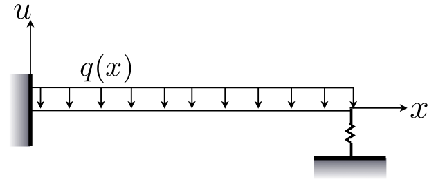
"Let us revisit the problem of the tensioned wire with elastic support, shown below\n",
"\n",
"\n",
"\n",
"The boundary condition at $x=L$ becomes $F=ku_L$, where, by balancing torque\n",
"\n",
"$$\n",
"F = \\frac{1}{L} \\int_0^L x q(x) dx\n",
"$$\n",
"\n",
"In this case, neither $u$ nor $u'$ is known at $x=L$. If we substitute $q(x) = -T u''(x)$, integration by parts gives\n",
"\n",
"$$\n",
"F = -\\frac{T}{L}\\left(L u'(L) - u(L)\\right) = T\\frac{u(L)}{L} - Tu'(L)\n",
"$$\n",
"\n",
"The boundary condition is of the form \n",
"\n",
"$$\n",
"\\alpha u + \\beta u' = \\gamma\n",
"$$\n",
"\n",
"where $\\alpha$, $\\beta$, and $\\gamma$ are known. The text (Ch 3.7) calls this type of boundary condition \"generalized boundary conditions\". This type of boundary condition arises in applications, such as convection, or elastic support of elastic bars.\n",
"\n",
"**Note:** prescribed displacements corresponds to $\\alpha=1$, $\\beta=0$ and prescribed force corresponds to $\\alpha=0$, $\\beta=1$.\n",
"\n",
"For the mixed case in which $\\beta$ is nonzero at both ends of the wire, the boundary conditions may be written\n",
"\n",
"$$\n",
"u'(0) = \\frac{\\gamma_0}{\\beta_0} - \\frac{\\alpha_0}{\\beta_0} u(0)\n",
"$$\n",
"$$\n",
"u'(L) = \\frac{\\gamma_L}{\\beta_L} - \\frac{\\alpha_L}{\\beta_L} u(L)\n",
"$$\n",
"\n",
"Substituting $u(x) = u_i \\phi_i(x)$ and $w(x) = w_i \\phi_i(x)$ eventually leads to the following system of equations for the unknown nodal displacements\n",
"\n",
"$$\n",
"K^*_{ij} u_j = f^*_i\n",
"$$\n",
"\n",
"where $K^*_{ij}$ and $f^*_i$ are the same as $K_{ij}$ and $f_i$ except\n",
"\n",
"$$\n",
"\\boxed{\n",
"\\begin{eqnarray}\n",
"K^*_{11} &= K_{11} - \\frac{\\alpha_0}{\\beta_0} \\\\\n",
"K^*_{NN} &= K_{NN} + \\frac{\\alpha_L}{\\beta_L} \\\\\n",
"f^*_{1} &= f_{1} - \\frac{\\gamma_0}{\\beta_0} \\\\\n",
"f^*_{N} &= f_{N} + \\frac{\\gamma_L}{\\beta_L}\n",
"\\end{eqnarray}\n",
"}\n",
"$$\n",
"\n",
"This holds for nonzero $\\beta_0$ and $\\beta_L$. In the case where $\\beta_0=\\beta_L=0$, replace $\\beta$ witha tiny number $(10^{-9})$ and the result will be the penalty method!\n",
"\n",
"This if boundary conditions are of general form, no special case coding is needed! Actually, supporting more complicated boundary conditions, in this case, actually simplifies the structure of the code.\n",
"\n",
"**Sidenote**\n",
"\n",
"A code should include a solvability check to ensure that\n",
"\n",
"- The number of prescribed displacements is $\\leq 2$\n",
"- Only one of $u$ or $u'$ is prescribed at any single boundary node"
]
},
{
"cell_type": "code",
"execution_count": null,
"metadata": {
"collapsed": true
},
"outputs": [],
"source": []
},
{
"cell_type": "markdown",
"metadata": {},
"source": [
"# Generalized Boundary Conditions\n",
"\n",
"1D equations for heat flow, diffusion and elasticity are all two‐point boundary problems of the form\n",
"\n",
"$$\n",
"\\frac{d}{dx}\\left(a \\frac{du}{dx}\\right) + bu + c = 0, \\quad \\text{on }\\Omega\n",
"$$\n",
"\n",
"We can introduce a **Generalized Boundary Condition** statement\n",
"\n",
"$$\n",
"\\left(\\alpha n \\frac{du}{dx}-\\overline{\\Phi}\\right) + \\beta\\left(u-\\overline{u}\\right)=0, \n",
"\\quad \\text{on } \\Gamma_{\\Phi}\n",
"$$\n",
"\n",
"With the penalty method, we can apply this condition to the entire domain boundary, selecting parameters to reduce this expression to Dirichlet, Neumann, or Robin boundary conditions.\n",
"\n",
"
\n",
"\n",
"The governing equation for this case is\n",
" \n",
"$$ T\\frac{d^2u}{d{x}^2}+q=0 $$\n",
"\n",
"$$ u(0)=0, \\qquad \\left( T\\frac{du}{dx}\\right)\\Bigg|_{x=L}=ku_L $$\n",
"\n",
"For a mesh of two linear elements, the global system of equations is:\n",
" \n",
"$$\n",
"\\frac{2T}{L}\\begin{pmatrix}\n",
"1 & -1 & 0 \\newline \n",
"-1 & 2 & -1 \\newline \n",
"0 & -1 & 1\n",
"\\end{pmatrix}\n",
"\\begin{pmatrix} \n",
"u_1 \\newline\n",
"u_2 \\newline\n",
"u_3 \n",
"\\end{pmatrix} \n",
"=\n",
"\\frac{qL}{4}\\begin{pmatrix}1 \\newline 2 \\newline 1 \\end{pmatrix} \n",
"+\n",
"\\begin{pmatrix} Q_1^1 \\newline Q_2^1+Q_1^2 \\newline Q_2^2 \\end{pmatrix}\n",
"$$\n",
"\n",
"Applying boundary conditions\n",
" \n",
"$$\n",
"\\frac{2T}{L}\\begin{pmatrix} \n",
"1 & -1 & 0 \\newline\n",
"-1 & 2 & -1 \\newline\n",
"0 & -1 & 1\n",
"\\end{pmatrix}\n",
"\\begin{pmatrix} \n",
"0 \\newline\n",
"u_2 \\newline\n",
"u_3 \\end{pmatrix} = \n",
"\\frac{qL}{4}\\begin{pmatrix}\n",
"1 \\newline\n",
"2 \\newline\n",
"1\n",
"\\end{pmatrix} +\n",
"\\begin{pmatrix} Q_1^1 \\newline 0 \\newline ku_3 \\end{pmatrix}\n",
"$$\n",
"\n",
"We re-write so that all unknowns are on the LHS:\n",
"$$\n",
"\\frac{2T}{L}\\begin{pmatrix}\n",
"1 & -1 & 0 \\newline\n",
" -1 & 2 & -1 \\newline\n",
" 0 & -1 & 1 - \\frac{kL}{2T} \\end{pmatrix}\n",
"\\begin{pmatrix} 0 \\newline \n",
"u_2 \\newline \n",
"u_3 \n",
"\\end{pmatrix}\n",
"=\n",
"\\frac{qL}{4}\\begin{pmatrix} \n",
"1 \\newline\n",
"2 \\newline\n",
"1\n",
"\\end{pmatrix} \n",
"+\n",
"\\begin{pmatrix} R_1 \\newline 0 \\newline 0 \\end{pmatrix}\n",
"$$\n",
"\n",
"The condensed equations are\n",
"\n",
"$$\n",
"\\frac{2T}{L}\\begin{pmatrix} \n",
"2 & -1 \\newline \n",
"-1 & 1-\\frac{kL}{2T} \\end{pmatrix}\n",
"\\begin{pmatrix} u_2 \\newline u_3 \\end{pmatrix} =\n",
"\\frac{qL}{4}\\begin{pmatrix} 2 \\newline 1 \\end{pmatrix}\n",
"$$\n",
"\n",
"which can then be solved for $u_2$ and $u_3$. We then find the reaction $R_1$\n",
"\n",
"$$\n",
" R_1=-\\frac{2T}{L}u_2-\\frac{qL}{2}\n",
"$$"
]
},
{
"cell_type": "markdown",
"metadata": {},
"source": [
"Let us revisit the problem of the tensioned wire with elastic support, shown below\n",
"\n",
"\n",
"\n",
"The boundary condition at $x=L$ becomes $F=ku_L$, where, by balancing torque\n",
"\n",
"$$\n",
"F = \\frac{1}{L} \\int_0^L x q(x) dx\n",
"$$\n",
"\n",
"In this case, neither $u$ nor $u'$ is known at $x=L$. If we substitute $q(x) = -T u''(x)$, integration by parts gives\n",
"\n",
"$$\n",
"F = -\\frac{T}{L}\\left(L u'(L) - u(L)\\right) = T\\frac{u(L)}{L} - Tu'(L)\n",
"$$\n",
"\n",
"The boundary condition is of the form \n",
"\n",
"$$\n",
"\\alpha u + \\beta u' = \\gamma\n",
"$$\n",
"\n",
"where $\\alpha$, $\\beta$, and $\\gamma$ are known. The text (Ch 3.7) calls this type of boundary condition \"generalized boundary conditions\". This type of boundary condition arises in applications, such as convection, or elastic support of elastic bars.\n",
"\n",
"**Note:** prescribed displacements corresponds to $\\alpha=1$, $\\beta=0$ and prescribed force corresponds to $\\alpha=0$, $\\beta=1$.\n",
"\n",
"For the mixed case in which $\\beta$ is nonzero at both ends of the wire, the boundary conditions may be written\n",
"\n",
"$$\n",
"u'(0) = \\frac{\\gamma_0}{\\beta_0} - \\frac{\\alpha_0}{\\beta_0} u(0)\n",
"$$\n",
"$$\n",
"u'(L) = \\frac{\\gamma_L}{\\beta_L} - \\frac{\\alpha_L}{\\beta_L} u(L)\n",
"$$\n",
"\n",
"Substituting $u(x) = u_i \\phi_i(x)$ and $w(x) = w_i \\phi_i(x)$ eventually leads to the following system of equations for the unknown nodal displacements\n",
"\n",
"$$\n",
"K^*_{ij} u_j = f^*_i\n",
"$$\n",
"\n",
"where $K^*_{ij}$ and $f^*_i$ are the same as $K_{ij}$ and $f_i$ except\n",
"\n",
"$$\n",
"\\boxed{\n",
"\\begin{eqnarray}\n",
"K^*_{11} &= K_{11} - \\frac{\\alpha_0}{\\beta_0} \\\\\n",
"K^*_{NN} &= K_{NN} + \\frac{\\alpha_L}{\\beta_L} \\\\\n",
"f^*_{1} &= f_{1} - \\frac{\\gamma_0}{\\beta_0} \\\\\n",
"f^*_{N} &= f_{N} + \\frac{\\gamma_L}{\\beta_L}\n",
"\\end{eqnarray}\n",
"}\n",
"$$\n",
"\n",
"This holds for nonzero $\\beta_0$ and $\\beta_L$. In the case where $\\beta_0=\\beta_L=0$, replace $\\beta$ witha tiny number $(10^{-9})$ and the result will be the penalty method!\n",
"\n",
"This if boundary conditions are of general form, no special case coding is needed! Actually, supporting more complicated boundary conditions, in this case, actually simplifies the structure of the code.\n",
"\n",
"**Sidenote**\n",
"\n",
"A code should include a solvability check to ensure that\n",
"\n",
"- The number of prescribed displacements is $\\leq 2$\n",
"- Only one of $u$ or $u'$ is prescribed at any single boundary node"
]
},
{
"cell_type": "code",
"execution_count": null,
"metadata": {
"collapsed": true
},
"outputs": [],
"source": []
},
{
"cell_type": "markdown",
"metadata": {},
"source": [
"# Generalized Boundary Conditions\n",
"\n",
"1D equations for heat flow, diffusion and elasticity are all two‐point boundary problems of the form\n",
"\n",
"$$\n",
"\\frac{d}{dx}\\left(a \\frac{du}{dx}\\right) + bu + c = 0, \\quad \\text{on }\\Omega\n",
"$$\n",
"\n",
"We can introduce a **Generalized Boundary Condition** statement\n",
"\n",
"$$\n",
"\\left(\\alpha n \\frac{du}{dx}-\\overline{\\Phi}\\right) + \\beta\\left(u-\\overline{u}\\right)=0, \n",
"\\quad \\text{on } \\Gamma_{\\Phi}\n",
"$$\n",
"\n",
"With the penalty method, we can apply this condition to the entire domain boundary, selecting parameters to reduce this expression to Dirichlet, Neumann, or Robin boundary conditions.\n",
"\n",
" For very large $\\beta$, $u=\\overline{u}$. | \n",
" For $\\beta=0$, $\\frac{du}{dx} = \\frac{\\Phi}{\\alpha}$. | \n",
"
\n",
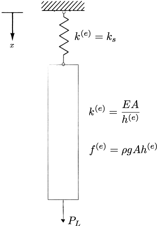
"Options for modeling a self‐weighted bar, supported by a spring\n",
"
\n",
"The generalized boundary condition approach can be extended to less trivial problems with elastic support and provides a more efficient method to defining the boundary interaction.\n",
" \n",
" | \n",
" \n",
" \n",
" \n",
" | \n",
"