# rayshader
 ## Overview
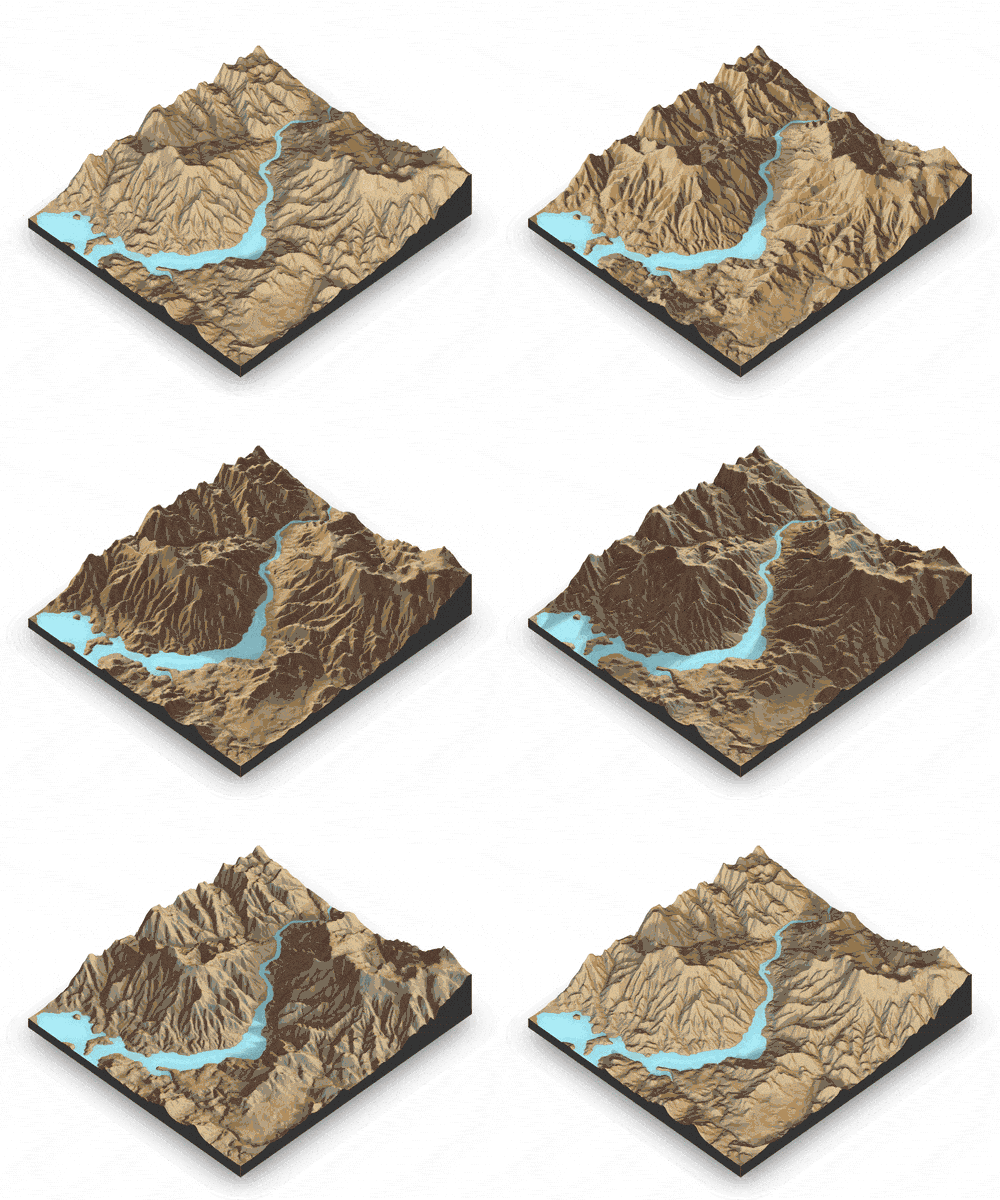
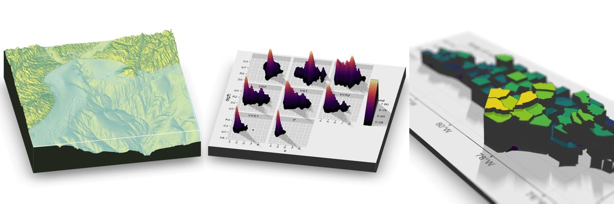
**rayshader** is an open source package for producing 2D and 3D data
visualizations in R. **rayshader** uses elevation data in a base R
matrix and a combination of raytracing, hillshading algorithms, and
overlays to generate stunning 2D and 3D maps. In addition to maps,
**rayshader** also allows the user to translate **ggplot2** objects into
beautiful 3D data visualizations.
The models can be rotated and examined interactively or the camera
movement can be scripted to create animations. Scenes can also be
rendered using a high-quality pathtracer, **rayrender**. The user can
also create a cinematic depth of field post-processing effect to direct
the user’s focus to important regions in the figure. The 3D models can
also be exported to a 3D-printable format with a built-in STL export
function, and can be exported to an OBJ file.
## Installation
``` r
# To install the latest version from Github:
# install.packages("devtools")
devtools::install_github("tylermorganwall/rayshader")
```
On Ubuntu, the following libraries are required:
``` bash
libpng-dev libjpeg-dev libfreetype6-dev libglu1-mesa-dev libgl1-mesa-dev pandoc zlib1g-dev libicu-dev libgdal-dev gdal-bin libgeos-dev libproj-dev
```
## Functions
## Overview
**rayshader** is an open source package for producing 2D and 3D data
visualizations in R. **rayshader** uses elevation data in a base R
matrix and a combination of raytracing, hillshading algorithms, and
overlays to generate stunning 2D and 3D maps. In addition to maps,
**rayshader** also allows the user to translate **ggplot2** objects into
beautiful 3D data visualizations.
The models can be rotated and examined interactively or the camera
movement can be scripted to create animations. Scenes can also be
rendered using a high-quality pathtracer, **rayrender**. The user can
also create a cinematic depth of field post-processing effect to direct
the user’s focus to important regions in the figure. The 3D models can
also be exported to a 3D-printable format with a built-in STL export
function, and can be exported to an OBJ file.
## Installation
``` r
# To install the latest version from Github:
# install.packages("devtools")
devtools::install_github("tylermorganwall/rayshader")
```
On Ubuntu, the following libraries are required:
``` bash
libpng-dev libjpeg-dev libfreetype6-dev libglu1-mesa-dev libgl1-mesa-dev pandoc zlib1g-dev libicu-dev libgdal-dev gdal-bin libgeos-dev libproj-dev
```
## Functions
 Rayshader has seven functions related to mapping:
- `ray_shade()` uses user specified light directions to calculate a
global shadow map for an elevation matrix. By default, this also
scales the light intensity at each point by the dot product of the
mean ray direction and the surface normal (also implemented in
function `lamb_shade`, this can be turned off by setting
`lambert=FALSE`.
- `sphere_shade()` maps an RGB texture to a hillshade by spherical
mapping. A texture can be generated with the `create_texture`
function, or loaded from an image. `sphere_shade` also includes 7
built-in palettes: “imhof1”, “imhof2”, “imhof3”, imhof4”, “desert”,
“bw”, “unicorn”.
- `ambient_shade()` creates an ambient occlusion shadow layer, darkening
areas that have less scattered light from the atmosphere. This results
in valleys being darker than flat areas and ridges.
- `texture_shade()` calculates a shadow for each point on the surface
using the method described by Leland Brown in “Texture Shading: A New
Technique for Depicting Terrain Relief.”
- `height_shade()` calculates a color for each point on the surface
using a direct elevation-to-color mapping.
- `lamb_shade()` uses a single user specified light direction to
calculate a local shadow map based on the dot product between the
surface normal and the light direction for an elevation matrix.
- `add_shadow()` takes two of the shadow maps above and combines them,
scaling the second one (or, if the second is an RGB array, the matrix)
as specified by the user.
- `add_overlay()` takes a 3 or 4-layer RGB/RGBA array and overlays it on
the current map. If the map includes transparency, this is taken into
account when overlaying the image. Otherwise, the user can specify a
single color that will be marked as completely transparent, or set the
full overlay as partly transparent.
- `create_texture()` programmatically creates texture maps given five
colors: a highlight, a shadow, a left fill light, a right fill light,
and a center color for flat areas. The user can also optionally
specify the colors at the corners, but `create_texture` will
interpolate those if they aren’t given.
Rayshader also has functions to add water and generate overlays:
- `detect_water()` uses a flood-fill algorithm to detect bodies of water
of a user-specified minimum area.
- `add_water()` uses the output of `detect_water` to add a water color
to the map. The user can input their own color, or pass the name of
one of the pre-defined palettes from `sphere_shade` to get a matching
hue.
- `generate_altitude_overlay()` uses a hillshade and the height map to
generate a semi-transparent hillshade whose transparency varies with
altitude.
- `generate_compass_overlay()` generates an overlay with a compass.
- `generate_contour_overlay()` calculates and returns an overlay of
contour lines.
- `generate_label_overlay()` this uses the `maptools::placeLabel()`
function to generate labels for the given scene. Either use an `sf`
object or manually specify the x/y coordinates and label.
- `generate_line_overlay()` generates an overlay of lines, using an `sf`
object with LINESTRING geometry.
- `generate_point_overlay()` generates an overlay of points, using an
`sf` object with POINT geometry.
- `generate_polygon_overlay()` generates an overlay of points, using an
`sf` object with POLYGON geometry.
- `generate_scalebar_overlay()` this function creates an overlay with a
scale bar of a user-specified length. It uses the coordinates of the
map (specified by passing an extent) and then creates a scale bar at a
specified x/y proportion across the map. If the map is not projected
(i.e. is in lat/long coordinates) this function will use the
`geosphere` package to create a scale bar of the proper length.
- `generate_waterline_overlay()` generates a semi-transparent waterline
overlay to layer onto an existing map using a height map or a boolean
matrix.
Also included are functions to add additional effects and information to
your 3D visualizations:
- `render_highquality()` renders in the scene with a built-in
pathtracer, powered by the **rayrender** package. Use this for
high-quality maps with realistic light transport.
- `render_depth()` generates a depth of field effect for the 3D map. The
user can specify the focal distance, focal length, and f-stop of the
camera, as well as aperture shape and bokeh intensity. This either
plots the image to the local device, or saves it to a file if given a
filename.
- `render_label()` adds a text label to the `x` and `y` coordinate of
the map at a specified altitude `z` (in units of the matrix). The
altitude can either be specified relative to the elevation at that
point (the default), or absolutely.
- `render_water()` adds a 3D tranparent water layer to 3D maps, after
the rgl device has already been created. This can either add to a map
that does not already have a water layer, or replace an existing water
layer on the map.
- `render_compass()` places a compass on the map in 3D.
- `render_path()` adds a 3D path to the current scene, using
latitude/longitude or coordinates in the reference system defined by
the extent object. If no altitude is provided, the path will be
elevated a constant offset above the heightmap.
- `render_points()` Adds 3D points to the current scene, using
latitude/longitude or coordinates in the reference system defined by
the extent object. If no altitude is provided, the points will be
elevated a constant offset above the heightmap.
- `render_polygons()` Adds 3D polygons to the current scene, using
latitude/longitude or coordinates in the reference system defined by
the extent object.
- `render_scalebar()` places a scalebar on the map in 3D.
And several helper functions for converting rasters to matrices:
- `raster_to_matrix()` converts a `raster` objects into a matrix.
- `resize_matrix()` resizes a matrix (preserving contents) by specifying
the desired output dimensions or a scaling factor.
And four functions to display and save your visualizations:
- `plot_map()` Plots the current map. Accepts either a matrix or an
array.
- `write_png()` Writes the current map to disk with a user-specified
filename.
- `plot_3d()` Creates a 3D map, given a texture and an elevation matrix.
You can customize the appearance of the map, as well as add a
user-defined water level.
- `render_camera()` Changes the camera orientation.
- `render_snapshot()` Saves an image of the current 3D view to disk (if
given a filename), or plots the 3D view to the current device (useful
for including images in R Markdown files).
- `render_movie()` Creates and saves a mp4/gif file of the camera
rotating around the 3D scene by either using a built-in orbit or by
using one provided by the user.
Finally, rayshader has a single function to generate 3D plots using
ggplot2 objects:
- `plot_gg()` Takes a ggplot2 object (or a list of two ggplot2 objects)
and uses the fill or color aesthetic to transform the plot into a 3D
surface. You can pass any of the arguments used to specify the camera
and the background/shadow colors in `plot_3d()`, and manipulate the
displayed 3D plot using `render_camera()` and `render_depth()`.
## Usage
Rayshader can be used for two purposes: both creating hillshaded maps
and 3D data visualizations plots. First, let’s look at rayshader’s
mapping capabilities. For the latter, scroll below.
## Mapping with rayshader
``` r
library(rayshader)
#Here, I load a map with the raster package.
loadzip = tempfile()
download.file("https://tylermw.com/data/dem_01.tif.zip", loadzip)
localtif = raster::raster(unzip(loadzip, "dem_01.tif"))
unlink(loadzip)
#And convert it to a matrix:
elmat = raster_to_matrix(localtif)
#We use another one of rayshader's built-in textures:
elmat |>
sphere_shade(texture = "desert") |>
plot_map()
```
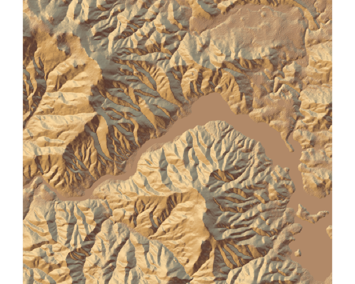
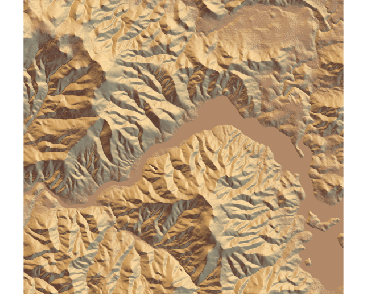
``` r
#sphere_shade can shift the sun direction:
elmat |>
sphere_shade(sunangle = 45, texture = "desert") |>
plot_map()
```
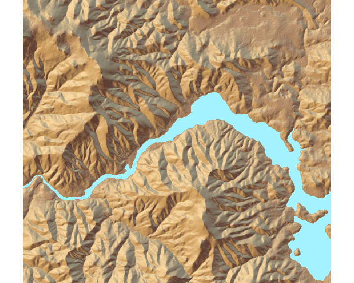
``` r
#detect_water and add_water adds a water layer to the map:
elmat |>
sphere_shade(texture = "desert") |>
add_water(detect_water(elmat), color = "desert") |>
plot_map()
```
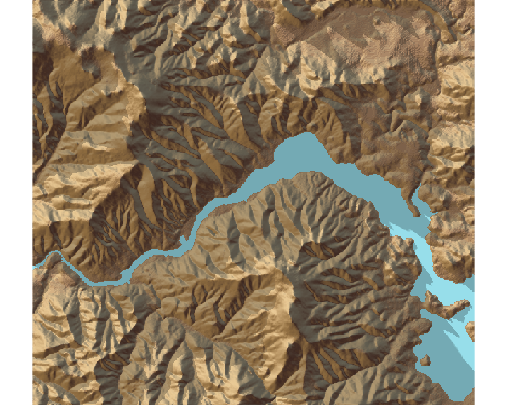
``` r
#And we can add a raytraced layer from that sun direction as well:
elmat |>
sphere_shade(texture = "desert") |>
add_water(detect_water(elmat), color = "desert") |>
add_shadow(ray_shade(elmat), 0.5) |>
plot_map()
```
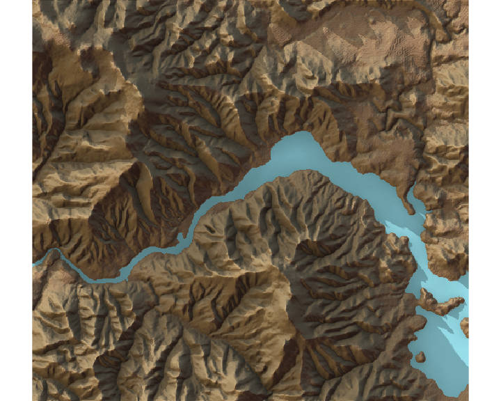
``` r
#And here we add an ambient occlusion shadow layer, which models
#lighting from atmospheric scattering:
elmat |>
sphere_shade(texture = "desert") |>
add_water(detect_water(elmat), color = "desert") |>
add_shadow(ray_shade(elmat), 0.5) |>
add_shadow(ambient_shade(elmat, maxsearch = 30), 0) |>
plot_map()
```
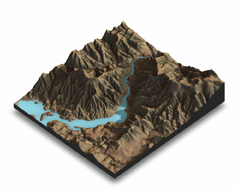
Rayshader also supports 3D mapping by passing a texture map (either
external or one produced by rayshader) into the `plot_3d` function.
``` r
elmat |>
sphere_shade(texture = "desert") |>
add_water(detect_water(elmat), color = "desert") |>
add_shadow(ray_shade(elmat, zscale = 3), 0.3) |>
add_shadow(ambient_shade(elmat), 0) |>
plot_3d(
elmat,
zscale = 10,
fov = 0,
theta = 135,
zoom = 0.75,
phi = 45,
windowsize = c(1000, 800)
)
Sys.sleep(0.2)
render_snapshot()
```
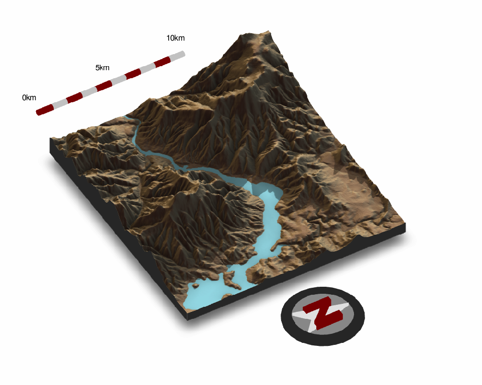
You can add a scale bar, as well as a compass using `render_scalebar()`
and `render_compass()`
``` r
render_camera(fov = 0, theta = 60, zoom = 0.75, phi = 45)
render_scalebar(
limits = c(0, 5, 10),
label_unit = "km",
position = "W",
y = 50,
scale_length = c(0.33, 1)
)
render_compass(position = "E")
render_snapshot(clear = TRUE)
```
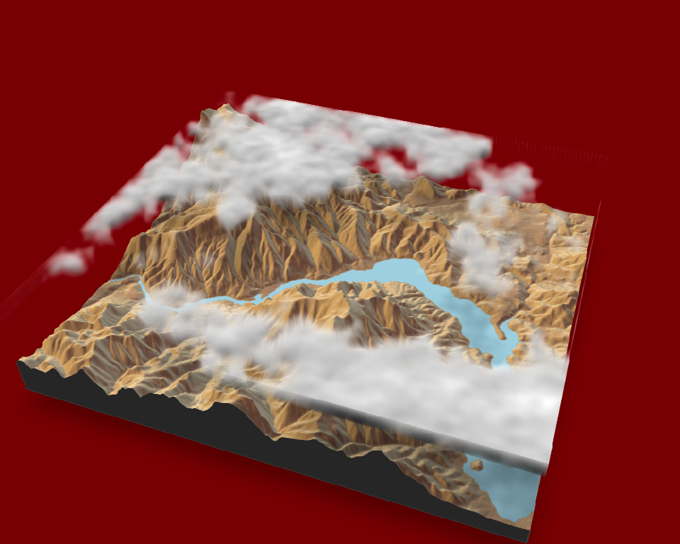
Rayshader also includes the option to add a procedurally-generated cloud
layer (and optionally, shadows):
``` r
elmat |>
sphere_shade(texture = "desert") |>
add_water(detect_water(elmat), color = "lightblue") |>
add_shadow(
cloud_shade(
elmat,
zscale = 10,
start_altitude = 500,
end_altitude = 1000,
),
0
) |>
plot_3d(
elmat,
zscale = 10,
fov = 0,
theta = 135,
zoom = 0.75,
phi = 45,
windowsize = c(1000, 800),
background = "darkred"
)
render_camera(theta = 20, phi = 40, zoom = 0.64, fov = 56)
render_clouds(
elmat,
zscale = 10,
start_altitude = 800,
end_altitude = 1000,
attenuation_coef = 5,
sun_altitude = 10,
clear_clouds = T
)
render_snapshot(clear = TRUE)
```
``` r
rgl::rgl.clear()
```
## Warning in rgl::rgl.clear(): 'rgl::rgl.clear' is deprecated.
## Use 'clear3d' instead.
## See help("Deprecated")
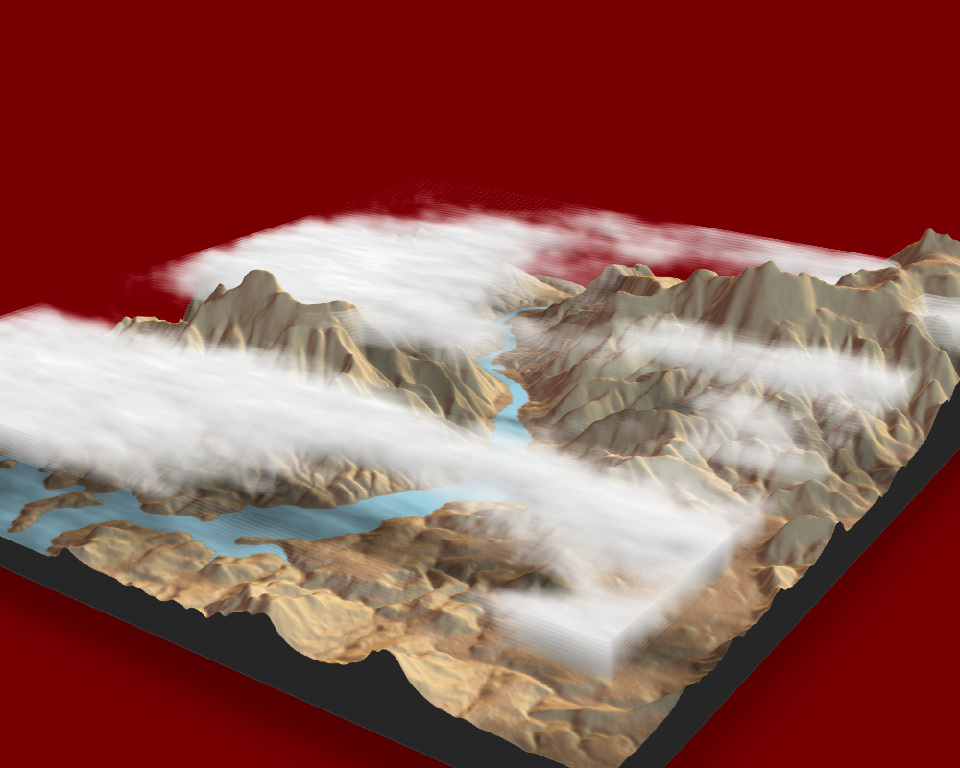
These clouds can be customized:
``` r
elmat |>
sphere_shade(texture = "desert") |>
add_water(detect_water(elmat), color = "lightblue") |>
add_shadow(
cloud_shade(
elmat,
zscale = 10,
start_altitude = 500,
end_altitude = 700,
sun_altitude = 45,
attenuation_coef = 2,
offset_y = 300,
cloud_cover = 0.55,
frequency = 0.01,
scale_y = 3,
fractal_levels = 32
),
0
) |>
plot_3d(
elmat,
zscale = 10,
fov = 0,
theta = 135,
zoom = 0.75,
phi = 45,
windowsize = c(1000, 800),
background = "darkred"
)
render_camera(theta = 125, phi = 22, zoom = 0.47, fov = 60)
render_clouds(
elmat,
zscale = 10,
start_altitude = 500,
end_altitude = 700,
sun_altitude = 45,
attenuation_coef = 2,
offset_y = 300,
cloud_cover = 0.55,
frequency = 0.01,
scale_y = 3,
fractal_levels = 32,
clear_clouds = T
)
render_snapshot(clear = TRUE)
```
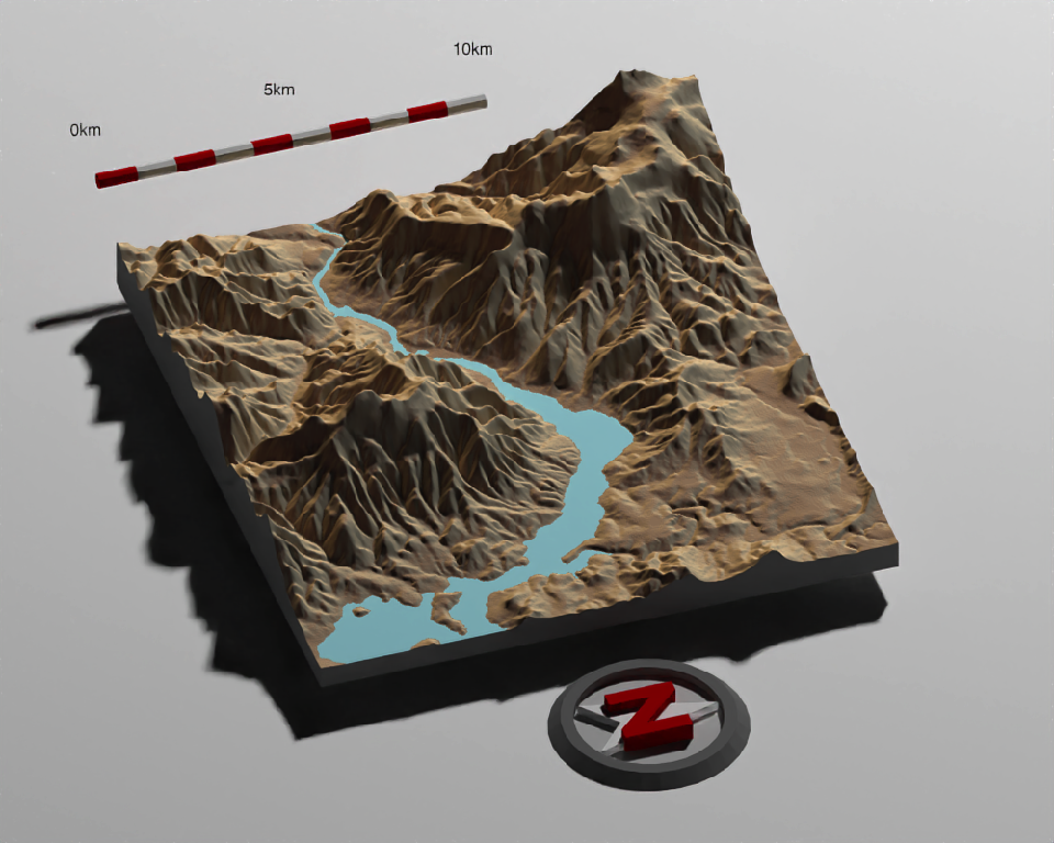
You can also render using the built-in pathtracer, powered by
[rayrender](https://www.rayrender.net). Simply replace
`render_snapshot()` with `render_highquality()`. When
`render_highquality()` is called, there’s no need to pre-compute the
shadows with any of the `_shade()` functions, so we remove those:
``` r
elmat |>
sphere_shade(texture = "desert") |>
add_water(detect_water(elmat), color = "desert") |>
plot_3d(
elmat,
zscale = 10,
fov = 0,
theta = 72,
zoom = 0.68,
phi = 40,
shadowdepth = -100,
soliddepth = -100,
windowsize = c(1000, 800)
)
render_scalebar(
limits = c(0, 5, 10),
label_unit = "km",
position = "W",
y = 50,
scale_length = c(0.33, 1)
)
render_compass(position = "E")
Sys.sleep(0.2)
render_highquality(samples = 16, scale_text_size = 24)
```
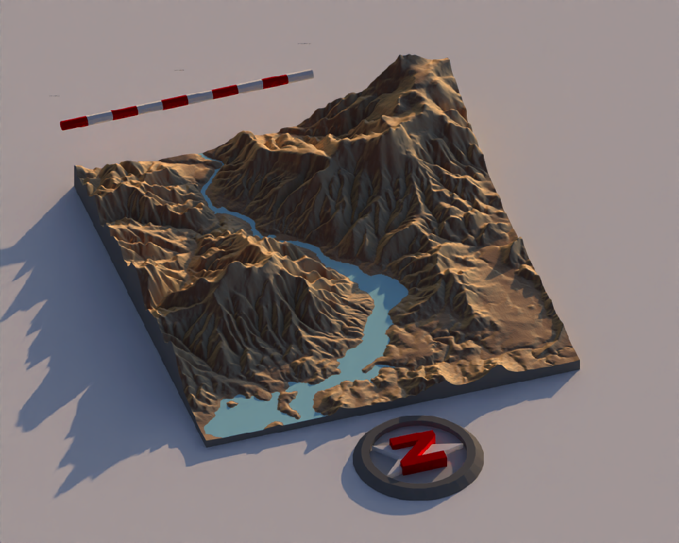
You can pass a latitude, longitude, and datetime to render this location
with a realistic atmosphere and sun direction at that time and place,
using the `skymodelr` package. Here’s Hobart, Tasmania in the winter in
the southern hemisphere.
``` r
elmat_lat_long = c(-42.745792, 147.171103)
render_highquality(
samples = 16,
lat = elmat_lat_long[1],
long = elmat_lat_long[2],
iso = 5, clamp_value = 1000,
datetime = as.POSIXct("2025-06-21 15:00:00", tz = "Australia/Sydney"),
sky_args = list(hosek = FALSE),
width=1000, height=800
)
```
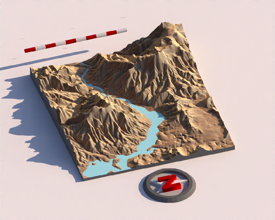
Here’s the same location at noon. This is the southern hemisphere, so
the light is coming from north, as noted by the compass.
``` r
render_highquality(
samples = 16,
lat = elmat_lat_long[1],
long = elmat_lat_long[2],
iso = 5, clamp_value = 1000,
datetime = as.POSIXct("2025-06-21 12:00:00", tz = "Australia/Sydney"),
sky_args = list(hosek = FALSE),
width=1000, height=800
)
```
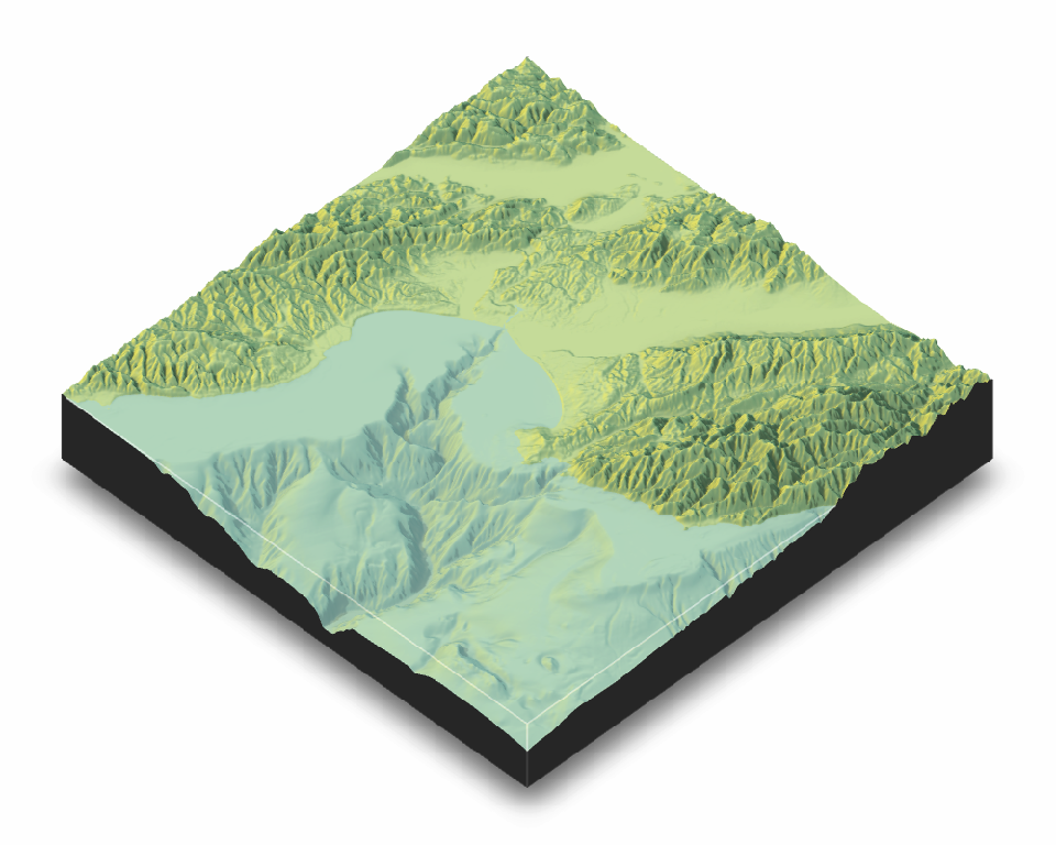
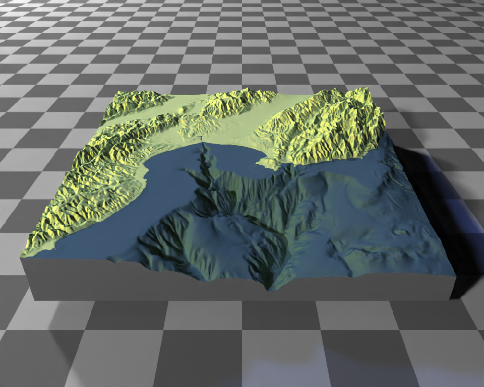
You can also easily add a water layer by setting `water = TRUE` in
`plot_3d()` (and setting `waterdepth` if the water level is not 0), or
by using the function `render_water()` after the 3D map has been
rendered. You can customize the appearance and transparancy of the water
layer via function arguments. Here’s an example using
bathymetric/topographic data of Monterey Bay, CA (included with
rayshader):
``` r
montshadow = ray_shade(montereybay, zscale = 50, lambert = FALSE)
montamb = ambient_shade(montereybay, zscale = 50)
montereybay |>
sphere_shade(zscale = 10, texture = "imhof1") |>
add_shadow(montshadow, 0.5) |>
add_shadow(montamb, 0) |>
plot_3d(
montereybay,
zscale = 50,
fov = 0,
theta = -45,
phi = 45,
windowsize = c(1000, 800),
zoom = 0.75,
water = TRUE,
waterdepth = 0,
wateralpha = 0.5,
watercolor = "lightblue",
waterlinecolor = "white",
waterlinealpha = 0.5
)
Sys.sleep(0.2)
render_snapshot(clear = TRUE)
```
Water is also supported in `render_highquality()`. We load the
`rayrender` package to change the ground material to include a checker
pattern. By default, the camera looks at the origin, but we shift it
down slightly to center the map.
``` r
library(rayrender)
```
##
## Attaching package: 'rayrender'
## The following object is masked from 'package:rayshader':
##
## run_documentation
## The following object is masked from 'package:rgl':
##
## text3d
``` r
montereybay |>
sphere_shade(zscale = 10, texture = "imhof1") |>
plot_3d(
montereybay,
zscale = 50,
fov = 70,
theta = 270,
phi = 30,
windowsize = c(1000, 800),
zoom = 0.6,
water = TRUE,
waterdepth = 0,
wateralpha = 0.5,
watercolor = "#233aa1",
waterlinecolor = "white",
waterlinealpha = 0.5
)
Sys.sleep(0.2)
render_highquality(
lightdirection = c(-45, 45),
lightaltitude = 30,
samples = 16,
camera_lookat = c(0, -50, 0),
ground_material = diffuse(
color = "grey50",
checkercolor = "grey20",
checkerperiod = 100
),
clear = TRUE
)
```
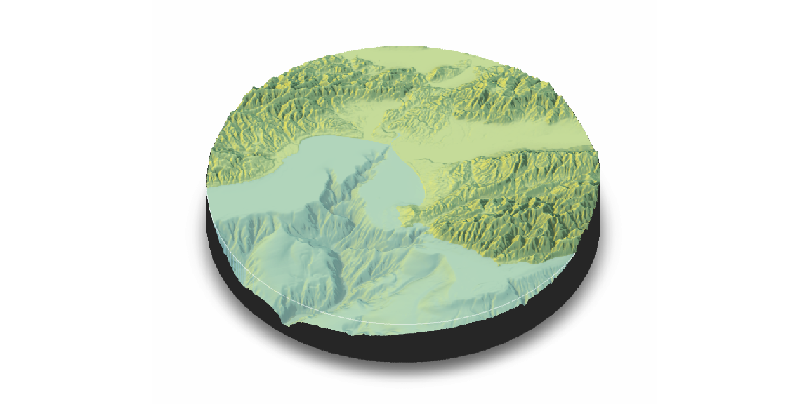
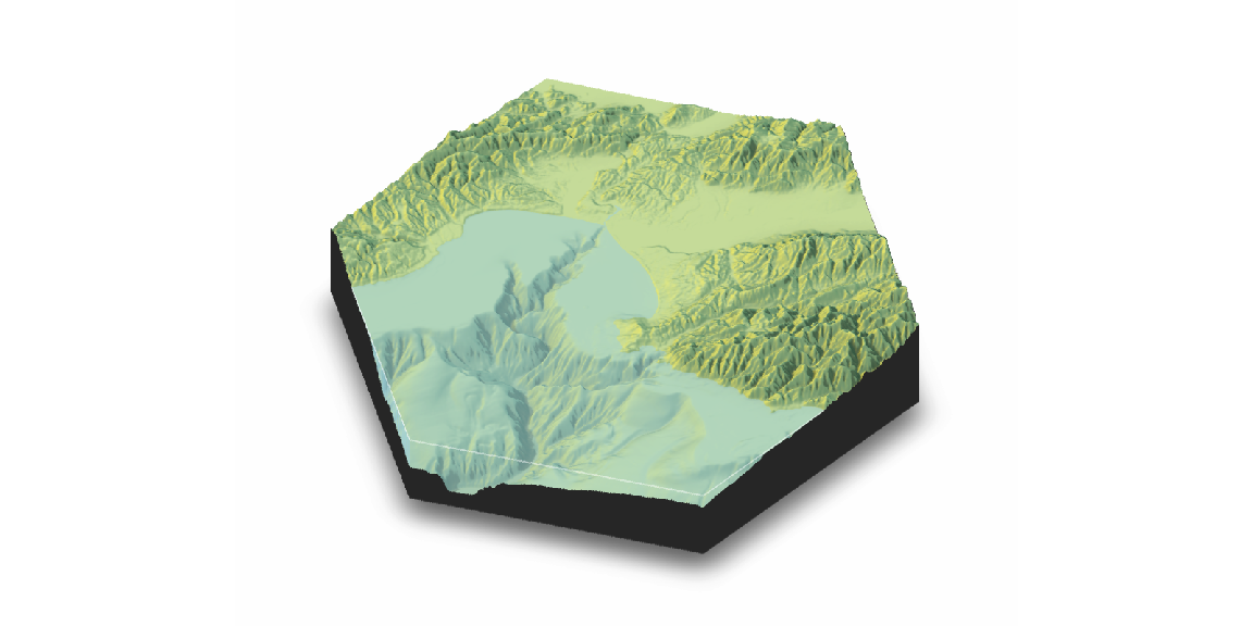
Rayshader also has map shapes other than rectangular included
`c("hex", "circle")`, and you can customize the map into any shape you
want by setting the areas you do not want to display to `NA`.
``` r
par(mfrow = c(1, 2))
montereybay |>
sphere_shade(zscale = 10, texture = "imhof1") |>
add_shadow(montshadow, 0.5) |>
add_shadow(montamb, 0) |>
plot_3d(
montereybay,
zscale = 50,
fov = 0,
theta = -45,
phi = 45,
windowsize = c(1000, 800),
zoom = 0.6,
water = TRUE,
waterdepth = 0,
wateralpha = 0.5,
watercolor = "lightblue",
waterlinecolor = "white",
waterlinealpha = 0.5,
baseshape = "circle"
)
render_snapshot(clear = TRUE)
```
``` r
montereybay |>
sphere_shade(zscale = 10, texture = "imhof1") |>
add_shadow(montshadow, 0.5) |>
add_shadow(montamb, 0) |>
plot_3d(
montereybay,
zscale = 50,
fov = 0,
theta = -45,
phi = 45,
windowsize = c(1000, 800),
zoom = 0.6,
water = TRUE,
waterdepth = 0,
wateralpha = 0.5,
watercolor = "lightblue",
waterlinecolor = "white",
waterlinealpha = 0.5,
baseshape = "hex"
)
render_snapshot(clear = TRUE)
```
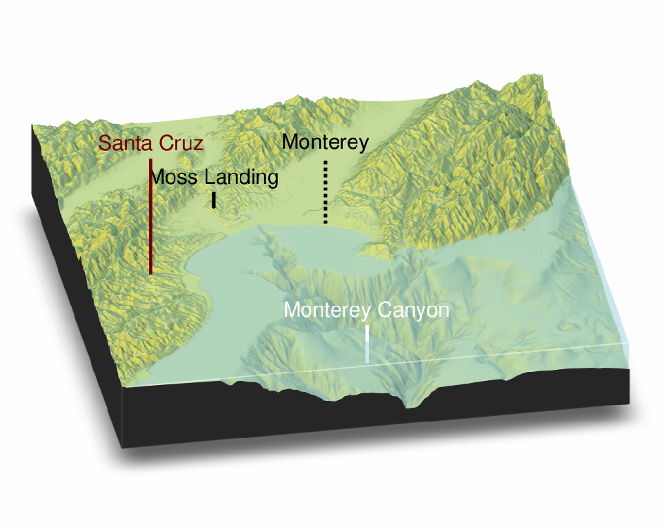
Adding text labels is done with the `render_label()` function, which
also allows you to customize the line type, color, and size along with
the font:
``` r
montereybay |>
sphere_shade(zscale = 10, texture = "imhof1") |>
add_shadow(montshadow, 0.5) |>
add_shadow(montamb, 0) |>
plot_3d(
montereybay,
zscale = 50,
fov = 0,
theta = -100,
phi = 30,
windowsize = c(1000, 800),
zoom = 0.6,
water = TRUE,
waterdepth = 0,
waterlinecolor = "white",
waterlinealpha = 0.5,
wateralpha = 0.5,
watercolor = "lightblue"
)
render_label(
montereybay,
x = 350,
y = 160,
z = 1000,
zscale = 50,
text = "Moss Landing",
textsize = 2,
linewidth = 5
)
render_label(
montereybay,
x = 220,
y = 70,
z = 7000,
zscale = 50,
text = "Santa Cruz",
textcolor = "darkred",
linecolor = "darkred",
textsize = 2,
linewidth = 5
)
render_label(
montereybay,
x = 300,
y = 270,
z = 4000,
zscale = 50,
text = "Monterey",
dashed = TRUE,
textsize = 2,
linewidth = 5
)
render_label(
montereybay,
x = 50,
y = 270,
z = 1000,
zscale = 50,
textcolor = "white",
linecolor = "white",
text = "Monterey Canyon",
relativez = FALSE,
textsize = 2,
linewidth = 5
)
Sys.sleep(0.2)
render_snapshot(clear = TRUE)
```
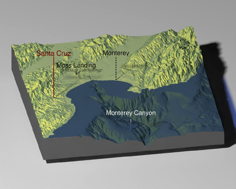
Labels are also supported in `render_highquality()`:
``` r
render_highquality(
samples = 16,
line_radius = 1,
text_size = 36,
text_offset = c(0, 12, 0),
clear = TRUE
)
```
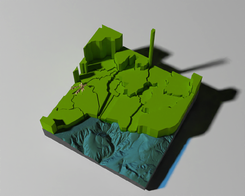
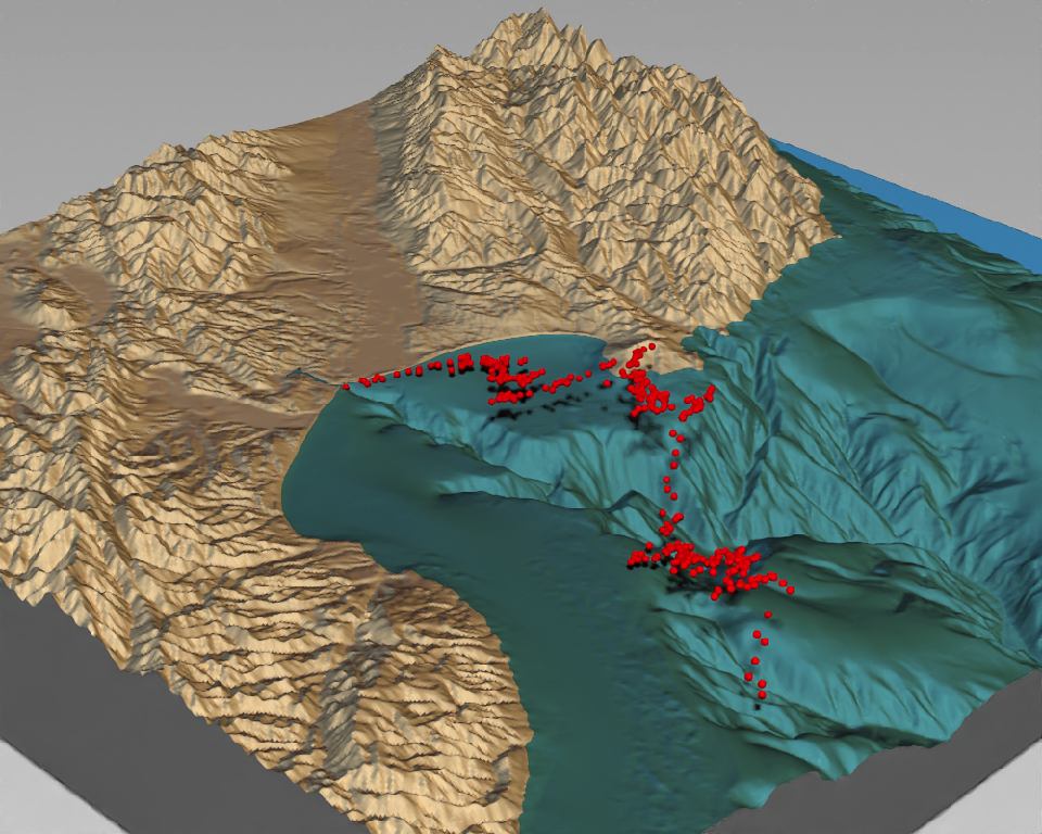
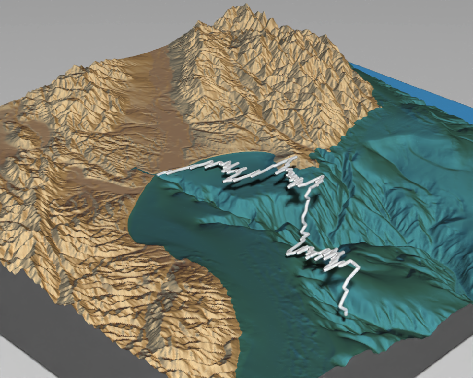
3D paths, points, and polygons can be added directly from spatial
objects from the `sf` library:
Polygons:
``` r
montereybay |>
sphere_shade(texture = "desert") |>
add_shadow(ray_shade(montereybay, zscale = 50)) |>
plot_3d(
montereybay,
water = TRUE,
windowsize = c(1000, 800),
watercolor = "dodgerblue"
)
render_camera(theta = -60, phi = 60, zoom = 0.85, fov = 30)
#We will apply a negative buffer to create space between adjacent polygons:
sf::sf_use_s2(FALSE)
mont_county_buff = sf::st_simplify(
sf::st_buffer(monterey_counties_sf, -0.003),
dTolerance = 0.004
)
render_polygons(
mont_county_buff,
extent = attr(montereybay, "extent"),
data_column_top = "ALAND",
scale_data = 300 / (2.6E9),
color = "chartreuse4",
parallel = TRUE
)
render_highquality(samples = 16)
```
``` r
render_polygons(clear_previous = TRUE)
render_camera(theta = 225, phi = 30, zoom = 0.37, fov = 48)
```
Points:
``` r
moss_landing_coord = c(36.806807, -121.793332)
x_vel_out = -0.0018 + rnorm(1000)[1:300] / 1000
y_vel_out = rnorm(1000)[1:300] / 100
z_out = c(
seq(0, 2000, length.out = 180),
seq(2000, 0, length.out = 10),
seq(0, 2000, length.out = 100),
seq(2000, 0, length.out = 10)
)
bird_track_lat = list()
bird_track_long = list()
bird_track_lat[[1]] = moss_landing_coord[1]
bird_track_long[[1]] = moss_landing_coord[2]
for (i in 2:300) {
bird_track_lat[[i]] = bird_track_lat[[i - 1]] + y_vel_out[i]
bird_track_long[[i]] = bird_track_long[[i - 1]] + x_vel_out[i]
}
render_points(
extent = attr(montereybay, "extent"),
lat = unlist(bird_track_lat),
long = unlist(bird_track_long),
altitude = z_out,
zscale = 50,
size = 3,
color = "red",
clear_previous = TRUE
)
render_highquality(point_radius = 0.5, samples = 16)
```
``` r
render_points(clear_previous = TRUE)
```
Paths:
``` r
render_path(
extent = attr(montereybay, "extent"),
lat = unlist(bird_track_lat),
long = unlist(bird_track_long),
altitude = z_out,
zscale = 50,
linewidth = 3,
color = "white",
antialias = TRUE
)
render_highquality(
line_radius = 0.5,
samples = 16,
clear = TRUE,
use_extruded_paths = TRUE
)
```
## Warning in mesh3d_model(mesh, x = x, y = y, z = z, override_material = TRUE, :
## material set as vertex color but no texture or bump map passed--ignoring mesh3d
## material.
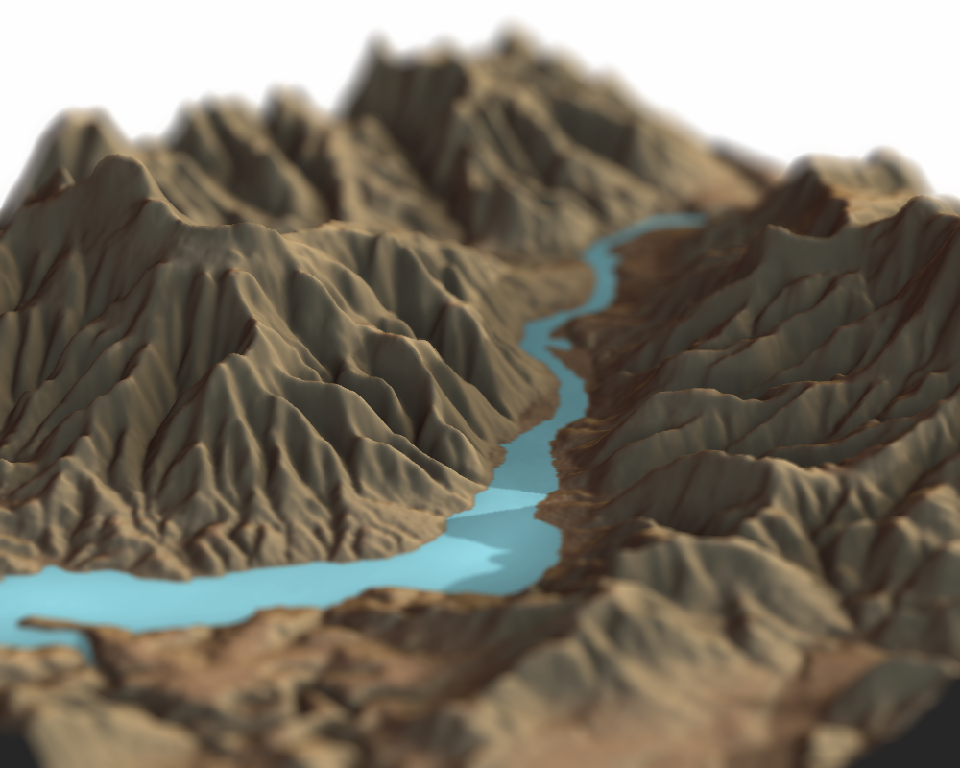
You can also apply a post-processing effect to the 3D maps to render
maps with depth of field with the `render_depth()` function:
``` r
elmat |>
sphere_shade(texture = "desert") |>
add_water(detect_water(elmat), color = "desert") |>
add_shadow(ray_shade(elmat, zscale = 3), 0.5) |>
add_shadow(ambient_shade(elmat), 0) |>
plot_3d(
elmat,
zscale = 10,
fov = 30,
theta = -225,
phi = 25,
windowsize = c(1000, 800),
zoom = 0.3
)
Sys.sleep(0.2)
render_depth(focallength = 800, clear = TRUE) #THIS NEEDS FIXING
```
## Focus distance: 1733.9
## 3D plotting with rayshader and ggplot2
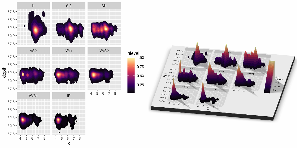
Rayshader can also be used to make 3D plots out of ggplot2 objects using
the `plot_gg()` function. Here, I turn a color density plot into a 3D
density plot. `plot_gg()` detects that the user mapped the `fill`
aesthetic to color and uses that information to project the figure into
3D.
``` r
library(ggplot2)
```
##
## Attaching package: 'ggplot2'
## The following object is masked from 'package:rayrender':
##
## arrow
``` r
ggdiamonds = ggplot(diamonds, aes(x, depth)) +
stat_density_2d(
aes(fill = after_stat(nlevel), color = after_stat(nlevel)),
geom = "polygon",
n = 200,
bins = 50,
contour = TRUE
) +
facet_wrap(clarity ~ .) +
scale_fill_viridis_c(option = "A") +
scale_color_viridis_c(option = "A")
# Return a preview snapshot
gg1 = plot_gg(
ggdiamonds,
width = 5,
height = 5,
raytrace = FALSE,
preview = TRUE
)
```
``` r
# Plot in 3D
plot_gg(
ggdiamonds,
width = 5,
height = 5,
multicore = TRUE,
scale = 250,
zoom = 0.7,
theta = 10,
phi = 30,
windowsize = c(800, 800)
)
Sys.sleep(0.2)
gg2 = render_snapshot(clear = TRUE, plot = FALSE)
```
``` r
rayimage::plot_image_grid(list(gg1, gg2), dim = c(1, 2))
```
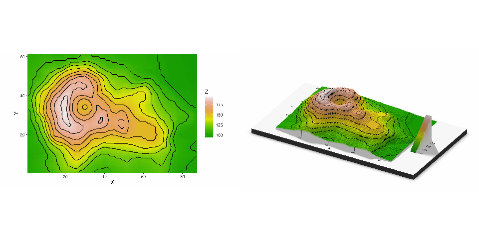
Rayshader will automatically ignore lines and other elements that should
not be mapped to 3D. Here’s a contour plot of the `volcano` dataset.
``` r
library(reshape2)
#Contours and other lines will automatically be ignored. Here is the volcano dataset:
ggvolcano = volcano |>
melt() |>
ggplot() +
geom_tile(aes(x = Var1, y = Var2, fill = value)) +
geom_contour(aes(x = Var1, y = Var2, z = value), color = "black") +
scale_x_continuous("X", expand = c(0, 0)) +
scale_y_continuous("Y", expand = c(0, 0)) +
scale_fill_gradientn("Z", colours = terrain.colors(10)) +
coord_fixed()
# Return a preview snapshot
gg3 = plot_gg(
ggvolcano,
width = 7,
height = 4,
raytrace = FALSE,
preview = TRUE
)
```
## Warning: Removed 1861 rows containing missing values or values outside the scale range
## (`geom_contour()`).
``` r
# Plot in 3D
plot_gg(
ggvolcano,
multicore = TRUE,
raytrace = TRUE,
width = 7,
height = 4,
scale = 300,
windowsize = c(1400, 866),
zoom = 0.6,
phi = 30,
theta = 30
)
```
## Warning: Removed 1861 rows containing missing values or values outside the scale range
## (`geom_contour()`).
``` r
Sys.sleep(0.2)
gg4 = render_snapshot(clear = TRUE, plot = FALSE)
```
``` r
rayimage::plot_image_grid(list(gg3, gg4), dim = c(1, 2))
```
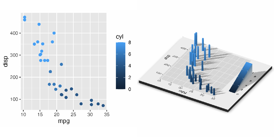
Rayshader also detects when the user passes the `color` aesthetic, and
maps those values to 3D. If both `color` and `fill` are passed, however,
rayshader will default to `fill`.
``` r
mtplot = ggplot(mtcars) +
geom_point(aes(x = mpg, y = disp, color = cyl), size = 2) +
scale_color_continuous(limits = c(0, 8))
# Return a preview snapshot
gg5 = plot_gg(mtplot, width = 3.5, raytrace = FALSE, preview = TRUE)
```
``` r
# Plot in 3D
plot_gg(
mtplot,
width = 3.5,
multicore = TRUE,
windowsize = c(800, 800),
zoom = 0.85,
phi = 35,
theta = 30,
sunangle = 225
)
Sys.sleep(0.2)
gg6 = render_snapshot(clear = TRUE, plot = FALSE)
```
``` r
rayimage::plot_image_grid(list(gg5, gg6), dim = c(1, 2))
```
Utilize combinations of line color and fill to create different effects.
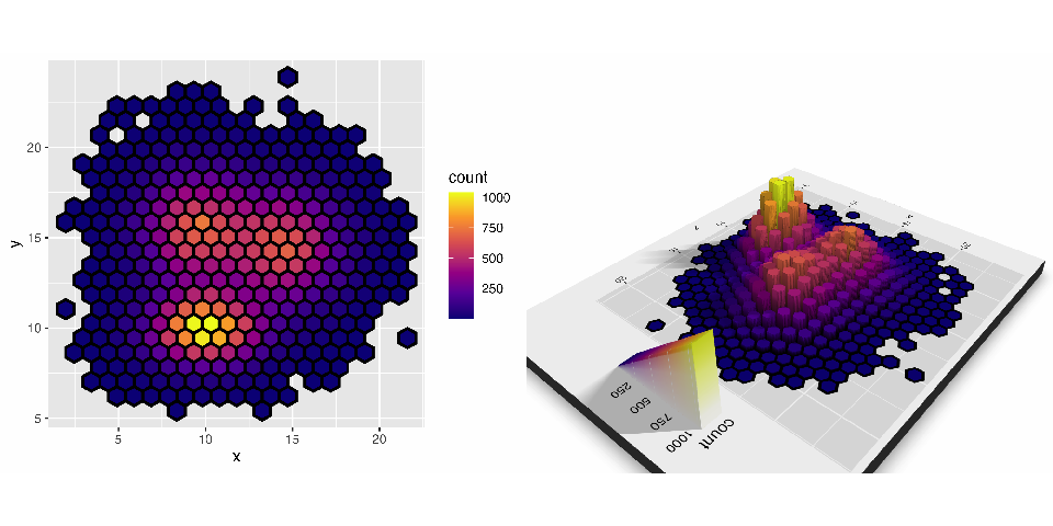
Here is a terraced hexbin plot, created by mapping the line colors of
the hexagons to black.
``` r
a = data.frame(x = rnorm(20000, 10, 1.9), y = rnorm(20000, 10, 1.2))
b = data.frame(x = rnorm(20000, 14.5, 1.9), y = rnorm(20000, 14.5, 1.9))
c = data.frame(x = rnorm(20000, 9.5, 1.9), y = rnorm(20000, 15.5, 1.9))
data = rbind(a, b, c)
#Lines
pp = ggplot(data, aes(x = x, y = y, fill = after_stat(count))) +
geom_hex(bins = 20, linewidth = 0.5, color = "black") +
scale_fill_viridis_c(option = "C") +
scale_color_viridis_c(option = "C")
gg7 = plot_gg(
pp,
width = 5,
height = 4,
scale = 300,
raytrace = FALSE,
preview = TRUE
)
```
``` r
plot_gg(
pp,
width = 5,
height = 4,
scale = 300,
multicore = TRUE,
windowsize = c(1000, 800)
)
render_camera(fov = 70, zoom = 0.5, theta = 130, phi = 35)
Sys.sleep(0.2)
gg8 = render_snapshot(clear = TRUE, plot = FALSE)
```
``` r
rayimage::plot_image_grid(list(gg7, gg8), dim = c(1, 2))
```
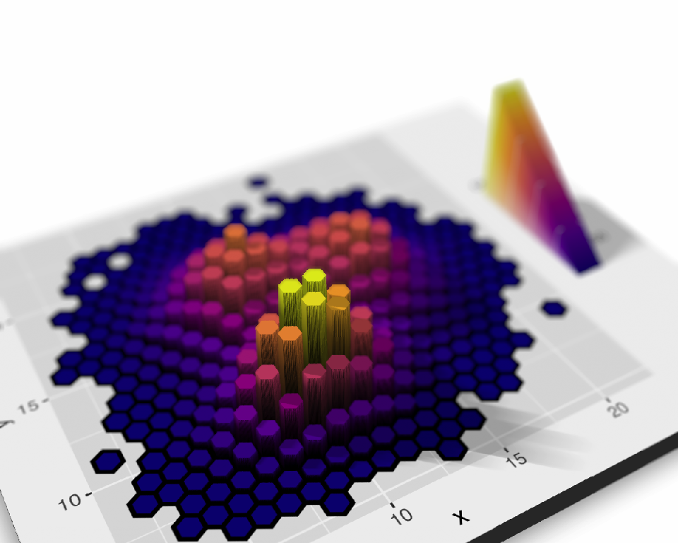
You can also use the `render_depth()` function to direct the viewer’s
focus to a important areas in the figure.
``` r
plot_gg(
pp,
width = 5,
height = 4,
scale = 300,
multicore = TRUE, offset_edges = 0,
windowsize = c(1200, 960),
fov = 70,
zoom = 0.4,
theta = 330,
phi = 40
)
Sys.sleep(0.2)
render_depth(focallength = 600, focus = 1700, clear = TRUE)
```
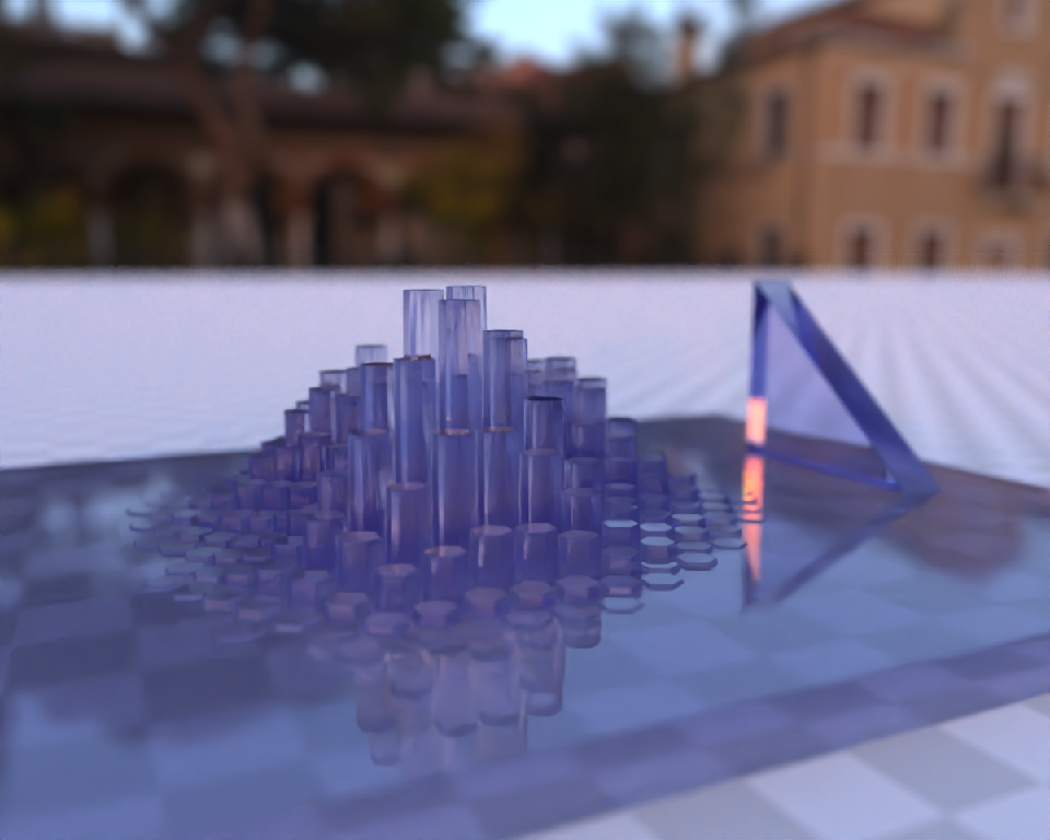
Finally, you can increase the allowable error in triangulating the model
to vastly reduce the size. Here, we reduce the model to 1/100th of it’s
raw (un-triangulated) size, while maintaining model quality. This can
improve the performance when rendering 3D ggplots with
`render_highquality()`, as well as improve performance on slower
computers. This triangulation is powered by the {terrainmeshr} package.
Here, we make a 3D ggplot out of glass, using a triangulated model and
`render_highquality()`.
``` r
tempfilehdr = tempfile(fileext = ".hdr")
download.file("https://www.tylermw.com/data/venice_sunset_2k.hdr", tempfilehdr)
par(mfrow = c(1, 1))
plot_gg(
pp,
width = 5,
height = 4,
scale = 300,
raytrace = FALSE,
windowsize = c(1200, 960),
fov = 129,
zoom = 0.21,
theta = -25,
phi = 9,
max_error = 0.01,
verbose = TRUE,
)
Sys.sleep(0.2)
render_highquality(
samples = 16,
aperture = 30,
light = FALSE,
override_material = TRUE,
focal_distance = 1043,
material = rayrender::dielectric(attenuation = c(1, 1, 0.3) / 200),
ground_material = rayrender::diffuse(
checkercolor = "grey80",
sigma = 90,
checkerperiod = 100
),
environment_light = tempfilehdr,
rotate_env = 180
)
```
Rayshader has seven functions related to mapping:
- `ray_shade()` uses user specified light directions to calculate a
global shadow map for an elevation matrix. By default, this also
scales the light intensity at each point by the dot product of the
mean ray direction and the surface normal (also implemented in
function `lamb_shade`, this can be turned off by setting
`lambert=FALSE`.
- `sphere_shade()` maps an RGB texture to a hillshade by spherical
mapping. A texture can be generated with the `create_texture`
function, or loaded from an image. `sphere_shade` also includes 7
built-in palettes: “imhof1”, “imhof2”, “imhof3”, imhof4”, “desert”,
“bw”, “unicorn”.
- `ambient_shade()` creates an ambient occlusion shadow layer, darkening
areas that have less scattered light from the atmosphere. This results
in valleys being darker than flat areas and ridges.
- `texture_shade()` calculates a shadow for each point on the surface
using the method described by Leland Brown in “Texture Shading: A New
Technique for Depicting Terrain Relief.”
- `height_shade()` calculates a color for each point on the surface
using a direct elevation-to-color mapping.
- `lamb_shade()` uses a single user specified light direction to
calculate a local shadow map based on the dot product between the
surface normal and the light direction for an elevation matrix.
- `add_shadow()` takes two of the shadow maps above and combines them,
scaling the second one (or, if the second is an RGB array, the matrix)
as specified by the user.
- `add_overlay()` takes a 3 or 4-layer RGB/RGBA array and overlays it on
the current map. If the map includes transparency, this is taken into
account when overlaying the image. Otherwise, the user can specify a
single color that will be marked as completely transparent, or set the
full overlay as partly transparent.
- `create_texture()` programmatically creates texture maps given five
colors: a highlight, a shadow, a left fill light, a right fill light,
and a center color for flat areas. The user can also optionally
specify the colors at the corners, but `create_texture` will
interpolate those if they aren’t given.
Rayshader also has functions to add water and generate overlays:
- `detect_water()` uses a flood-fill algorithm to detect bodies of water
of a user-specified minimum area.
- `add_water()` uses the output of `detect_water` to add a water color
to the map. The user can input their own color, or pass the name of
one of the pre-defined palettes from `sphere_shade` to get a matching
hue.
- `generate_altitude_overlay()` uses a hillshade and the height map to
generate a semi-transparent hillshade whose transparency varies with
altitude.
- `generate_compass_overlay()` generates an overlay with a compass.
- `generate_contour_overlay()` calculates and returns an overlay of
contour lines.
- `generate_label_overlay()` this uses the `maptools::placeLabel()`
function to generate labels for the given scene. Either use an `sf`
object or manually specify the x/y coordinates and label.
- `generate_line_overlay()` generates an overlay of lines, using an `sf`
object with LINESTRING geometry.
- `generate_point_overlay()` generates an overlay of points, using an
`sf` object with POINT geometry.
- `generate_polygon_overlay()` generates an overlay of points, using an
`sf` object with POLYGON geometry.
- `generate_scalebar_overlay()` this function creates an overlay with a
scale bar of a user-specified length. It uses the coordinates of the
map (specified by passing an extent) and then creates a scale bar at a
specified x/y proportion across the map. If the map is not projected
(i.e. is in lat/long coordinates) this function will use the
`geosphere` package to create a scale bar of the proper length.
- `generate_waterline_overlay()` generates a semi-transparent waterline
overlay to layer onto an existing map using a height map or a boolean
matrix.
Also included are functions to add additional effects and information to
your 3D visualizations:
- `render_highquality()` renders in the scene with a built-in
pathtracer, powered by the **rayrender** package. Use this for
high-quality maps with realistic light transport.
- `render_depth()` generates a depth of field effect for the 3D map. The
user can specify the focal distance, focal length, and f-stop of the
camera, as well as aperture shape and bokeh intensity. This either
plots the image to the local device, or saves it to a file if given a
filename.
- `render_label()` adds a text label to the `x` and `y` coordinate of
the map at a specified altitude `z` (in units of the matrix). The
altitude can either be specified relative to the elevation at that
point (the default), or absolutely.
- `render_water()` adds a 3D tranparent water layer to 3D maps, after
the rgl device has already been created. This can either add to a map
that does not already have a water layer, or replace an existing water
layer on the map.
- `render_compass()` places a compass on the map in 3D.
- `render_path()` adds a 3D path to the current scene, using
latitude/longitude or coordinates in the reference system defined by
the extent object. If no altitude is provided, the path will be
elevated a constant offset above the heightmap.
- `render_points()` Adds 3D points to the current scene, using
latitude/longitude or coordinates in the reference system defined by
the extent object. If no altitude is provided, the points will be
elevated a constant offset above the heightmap.
- `render_polygons()` Adds 3D polygons to the current scene, using
latitude/longitude or coordinates in the reference system defined by
the extent object.
- `render_scalebar()` places a scalebar on the map in 3D.
And several helper functions for converting rasters to matrices:
- `raster_to_matrix()` converts a `raster` objects into a matrix.
- `resize_matrix()` resizes a matrix (preserving contents) by specifying
the desired output dimensions or a scaling factor.
And four functions to display and save your visualizations:
- `plot_map()` Plots the current map. Accepts either a matrix or an
array.
- `write_png()` Writes the current map to disk with a user-specified
filename.
- `plot_3d()` Creates a 3D map, given a texture and an elevation matrix.
You can customize the appearance of the map, as well as add a
user-defined water level.
- `render_camera()` Changes the camera orientation.
- `render_snapshot()` Saves an image of the current 3D view to disk (if
given a filename), or plots the 3D view to the current device (useful
for including images in R Markdown files).
- `render_movie()` Creates and saves a mp4/gif file of the camera
rotating around the 3D scene by either using a built-in orbit or by
using one provided by the user.
Finally, rayshader has a single function to generate 3D plots using
ggplot2 objects:
- `plot_gg()` Takes a ggplot2 object (or a list of two ggplot2 objects)
and uses the fill or color aesthetic to transform the plot into a 3D
surface. You can pass any of the arguments used to specify the camera
and the background/shadow colors in `plot_3d()`, and manipulate the
displayed 3D plot using `render_camera()` and `render_depth()`.
## Usage
Rayshader can be used for two purposes: both creating hillshaded maps
and 3D data visualizations plots. First, let’s look at rayshader’s
mapping capabilities. For the latter, scroll below.
## Mapping with rayshader
``` r
library(rayshader)
#Here, I load a map with the raster package.
loadzip = tempfile()
download.file("https://tylermw.com/data/dem_01.tif.zip", loadzip)
localtif = raster::raster(unzip(loadzip, "dem_01.tif"))
unlink(loadzip)
#And convert it to a matrix:
elmat = raster_to_matrix(localtif)
#We use another one of rayshader's built-in textures:
elmat |>
sphere_shade(texture = "desert") |>
plot_map()
```

``` r
#sphere_shade can shift the sun direction:
elmat |>
sphere_shade(sunangle = 45, texture = "desert") |>
plot_map()
```

``` r
#detect_water and add_water adds a water layer to the map:
elmat |>
sphere_shade(texture = "desert") |>
add_water(detect_water(elmat), color = "desert") |>
plot_map()
```

``` r
#And we can add a raytraced layer from that sun direction as well:
elmat |>
sphere_shade(texture = "desert") |>
add_water(detect_water(elmat), color = "desert") |>
add_shadow(ray_shade(elmat), 0.5) |>
plot_map()
```

``` r
#And here we add an ambient occlusion shadow layer, which models
#lighting from atmospheric scattering:
elmat |>
sphere_shade(texture = "desert") |>
add_water(detect_water(elmat), color = "desert") |>
add_shadow(ray_shade(elmat), 0.5) |>
add_shadow(ambient_shade(elmat, maxsearch = 30), 0) |>
plot_map()
```

Rayshader also supports 3D mapping by passing a texture map (either
external or one produced by rayshader) into the `plot_3d` function.
``` r
elmat |>
sphere_shade(texture = "desert") |>
add_water(detect_water(elmat), color = "desert") |>
add_shadow(ray_shade(elmat, zscale = 3), 0.3) |>
add_shadow(ambient_shade(elmat), 0) |>
plot_3d(
elmat,
zscale = 10,
fov = 0,
theta = 135,
zoom = 0.75,
phi = 45,
windowsize = c(1000, 800)
)
Sys.sleep(0.2)
render_snapshot()
```

You can add a scale bar, as well as a compass using `render_scalebar()`
and `render_compass()`
``` r
render_camera(fov = 0, theta = 60, zoom = 0.75, phi = 45)
render_scalebar(
limits = c(0, 5, 10),
label_unit = "km",
position = "W",
y = 50,
scale_length = c(0.33, 1)
)
render_compass(position = "E")
render_snapshot(clear = TRUE)
```

Rayshader also includes the option to add a procedurally-generated cloud
layer (and optionally, shadows):
``` r
elmat |>
sphere_shade(texture = "desert") |>
add_water(detect_water(elmat), color = "lightblue") |>
add_shadow(
cloud_shade(
elmat,
zscale = 10,
start_altitude = 500,
end_altitude = 1000,
),
0
) |>
plot_3d(
elmat,
zscale = 10,
fov = 0,
theta = 135,
zoom = 0.75,
phi = 45,
windowsize = c(1000, 800),
background = "darkred"
)
render_camera(theta = 20, phi = 40, zoom = 0.64, fov = 56)
render_clouds(
elmat,
zscale = 10,
start_altitude = 800,
end_altitude = 1000,
attenuation_coef = 5,
sun_altitude = 10,
clear_clouds = T
)
render_snapshot(clear = TRUE)
```

``` r
rgl::rgl.clear()
```
## Warning in rgl::rgl.clear(): 'rgl::rgl.clear' is deprecated.
## Use 'clear3d' instead.
## See help("Deprecated")
These clouds can be customized:
``` r
elmat |>
sphere_shade(texture = "desert") |>
add_water(detect_water(elmat), color = "lightblue") |>
add_shadow(
cloud_shade(
elmat,
zscale = 10,
start_altitude = 500,
end_altitude = 700,
sun_altitude = 45,
attenuation_coef = 2,
offset_y = 300,
cloud_cover = 0.55,
frequency = 0.01,
scale_y = 3,
fractal_levels = 32
),
0
) |>
plot_3d(
elmat,
zscale = 10,
fov = 0,
theta = 135,
zoom = 0.75,
phi = 45,
windowsize = c(1000, 800),
background = "darkred"
)
render_camera(theta = 125, phi = 22, zoom = 0.47, fov = 60)
render_clouds(
elmat,
zscale = 10,
start_altitude = 500,
end_altitude = 700,
sun_altitude = 45,
attenuation_coef = 2,
offset_y = 300,
cloud_cover = 0.55,
frequency = 0.01,
scale_y = 3,
fractal_levels = 32,
clear_clouds = T
)
render_snapshot(clear = TRUE)
```

You can also render using the built-in pathtracer, powered by
[rayrender](https://www.rayrender.net). Simply replace
`render_snapshot()` with `render_highquality()`. When
`render_highquality()` is called, there’s no need to pre-compute the
shadows with any of the `_shade()` functions, so we remove those:
``` r
elmat |>
sphere_shade(texture = "desert") |>
add_water(detect_water(elmat), color = "desert") |>
plot_3d(
elmat,
zscale = 10,
fov = 0,
theta = 72,
zoom = 0.68,
phi = 40,
shadowdepth = -100,
soliddepth = -100,
windowsize = c(1000, 800)
)
render_scalebar(
limits = c(0, 5, 10),
label_unit = "km",
position = "W",
y = 50,
scale_length = c(0.33, 1)
)
render_compass(position = "E")
Sys.sleep(0.2)
render_highquality(samples = 16, scale_text_size = 24)
```

You can pass a latitude, longitude, and datetime to render this location
with a realistic atmosphere and sun direction at that time and place,
using the `skymodelr` package. Here’s Hobart, Tasmania in the winter in
the southern hemisphere.
``` r
elmat_lat_long = c(-42.745792, 147.171103)
render_highquality(
samples = 16,
lat = elmat_lat_long[1],
long = elmat_lat_long[2],
iso = 5, clamp_value = 1000,
datetime = as.POSIXct("2025-06-21 15:00:00", tz = "Australia/Sydney"),
sky_args = list(hosek = FALSE),
width=1000, height=800
)
```

Here’s the same location at noon. This is the southern hemisphere, so
the light is coming from north, as noted by the compass.
``` r
render_highquality(
samples = 16,
lat = elmat_lat_long[1],
long = elmat_lat_long[2],
iso = 5, clamp_value = 1000,
datetime = as.POSIXct("2025-06-21 12:00:00", tz = "Australia/Sydney"),
sky_args = list(hosek = FALSE),
width=1000, height=800
)
```

You can also easily add a water layer by setting `water = TRUE` in
`plot_3d()` (and setting `waterdepth` if the water level is not 0), or
by using the function `render_water()` after the 3D map has been
rendered. You can customize the appearance and transparancy of the water
layer via function arguments. Here’s an example using
bathymetric/topographic data of Monterey Bay, CA (included with
rayshader):
``` r
montshadow = ray_shade(montereybay, zscale = 50, lambert = FALSE)
montamb = ambient_shade(montereybay, zscale = 50)
montereybay |>
sphere_shade(zscale = 10, texture = "imhof1") |>
add_shadow(montshadow, 0.5) |>
add_shadow(montamb, 0) |>
plot_3d(
montereybay,
zscale = 50,
fov = 0,
theta = -45,
phi = 45,
windowsize = c(1000, 800),
zoom = 0.75,
water = TRUE,
waterdepth = 0,
wateralpha = 0.5,
watercolor = "lightblue",
waterlinecolor = "white",
waterlinealpha = 0.5
)
Sys.sleep(0.2)
render_snapshot(clear = TRUE)
```

Water is also supported in `render_highquality()`. We load the
`rayrender` package to change the ground material to include a checker
pattern. By default, the camera looks at the origin, but we shift it
down slightly to center the map.
``` r
library(rayrender)
```
##
## Attaching package: 'rayrender'
## The following object is masked from 'package:rayshader':
##
## run_documentation
## The following object is masked from 'package:rgl':
##
## text3d
``` r
montereybay |>
sphere_shade(zscale = 10, texture = "imhof1") |>
plot_3d(
montereybay,
zscale = 50,
fov = 70,
theta = 270,
phi = 30,
windowsize = c(1000, 800),
zoom = 0.6,
water = TRUE,
waterdepth = 0,
wateralpha = 0.5,
watercolor = "#233aa1",
waterlinecolor = "white",
waterlinealpha = 0.5
)
Sys.sleep(0.2)
render_highquality(
lightdirection = c(-45, 45),
lightaltitude = 30,
samples = 16,
camera_lookat = c(0, -50, 0),
ground_material = diffuse(
color = "grey50",
checkercolor = "grey20",
checkerperiod = 100
),
clear = TRUE
)
```

Rayshader also has map shapes other than rectangular included
`c("hex", "circle")`, and you can customize the map into any shape you
want by setting the areas you do not want to display to `NA`.
``` r
par(mfrow = c(1, 2))
montereybay |>
sphere_shade(zscale = 10, texture = "imhof1") |>
add_shadow(montshadow, 0.5) |>
add_shadow(montamb, 0) |>
plot_3d(
montereybay,
zscale = 50,
fov = 0,
theta = -45,
phi = 45,
windowsize = c(1000, 800),
zoom = 0.6,
water = TRUE,
waterdepth = 0,
wateralpha = 0.5,
watercolor = "lightblue",
waterlinecolor = "white",
waterlinealpha = 0.5,
baseshape = "circle"
)
render_snapshot(clear = TRUE)
```

``` r
montereybay |>
sphere_shade(zscale = 10, texture = "imhof1") |>
add_shadow(montshadow, 0.5) |>
add_shadow(montamb, 0) |>
plot_3d(
montereybay,
zscale = 50,
fov = 0,
theta = -45,
phi = 45,
windowsize = c(1000, 800),
zoom = 0.6,
water = TRUE,
waterdepth = 0,
wateralpha = 0.5,
watercolor = "lightblue",
waterlinecolor = "white",
waterlinealpha = 0.5,
baseshape = "hex"
)
render_snapshot(clear = TRUE)
```

Adding text labels is done with the `render_label()` function, which
also allows you to customize the line type, color, and size along with
the font:
``` r
montereybay |>
sphere_shade(zscale = 10, texture = "imhof1") |>
add_shadow(montshadow, 0.5) |>
add_shadow(montamb, 0) |>
plot_3d(
montereybay,
zscale = 50,
fov = 0,
theta = -100,
phi = 30,
windowsize = c(1000, 800),
zoom = 0.6,
water = TRUE,
waterdepth = 0,
waterlinecolor = "white",
waterlinealpha = 0.5,
wateralpha = 0.5,
watercolor = "lightblue"
)
render_label(
montereybay,
x = 350,
y = 160,
z = 1000,
zscale = 50,
text = "Moss Landing",
textsize = 2,
linewidth = 5
)
render_label(
montereybay,
x = 220,
y = 70,
z = 7000,
zscale = 50,
text = "Santa Cruz",
textcolor = "darkred",
linecolor = "darkred",
textsize = 2,
linewidth = 5
)
render_label(
montereybay,
x = 300,
y = 270,
z = 4000,
zscale = 50,
text = "Monterey",
dashed = TRUE,
textsize = 2,
linewidth = 5
)
render_label(
montereybay,
x = 50,
y = 270,
z = 1000,
zscale = 50,
textcolor = "white",
linecolor = "white",
text = "Monterey Canyon",
relativez = FALSE,
textsize = 2,
linewidth = 5
)
Sys.sleep(0.2)
render_snapshot(clear = TRUE)
```

Labels are also supported in `render_highquality()`:
``` r
render_highquality(
samples = 16,
line_radius = 1,
text_size = 36,
text_offset = c(0, 12, 0),
clear = TRUE
)
```

3D paths, points, and polygons can be added directly from spatial
objects from the `sf` library:
Polygons:
``` r
montereybay |>
sphere_shade(texture = "desert") |>
add_shadow(ray_shade(montereybay, zscale = 50)) |>
plot_3d(
montereybay,
water = TRUE,
windowsize = c(1000, 800),
watercolor = "dodgerblue"
)
render_camera(theta = -60, phi = 60, zoom = 0.85, fov = 30)
#We will apply a negative buffer to create space between adjacent polygons:
sf::sf_use_s2(FALSE)
mont_county_buff = sf::st_simplify(
sf::st_buffer(monterey_counties_sf, -0.003),
dTolerance = 0.004
)
render_polygons(
mont_county_buff,
extent = attr(montereybay, "extent"),
data_column_top = "ALAND",
scale_data = 300 / (2.6E9),
color = "chartreuse4",
parallel = TRUE
)
render_highquality(samples = 16)
```

``` r
render_polygons(clear_previous = TRUE)
render_camera(theta = 225, phi = 30, zoom = 0.37, fov = 48)
```
Points:
``` r
moss_landing_coord = c(36.806807, -121.793332)
x_vel_out = -0.0018 + rnorm(1000)[1:300] / 1000
y_vel_out = rnorm(1000)[1:300] / 100
z_out = c(
seq(0, 2000, length.out = 180),
seq(2000, 0, length.out = 10),
seq(0, 2000, length.out = 100),
seq(2000, 0, length.out = 10)
)
bird_track_lat = list()
bird_track_long = list()
bird_track_lat[[1]] = moss_landing_coord[1]
bird_track_long[[1]] = moss_landing_coord[2]
for (i in 2:300) {
bird_track_lat[[i]] = bird_track_lat[[i - 1]] + y_vel_out[i]
bird_track_long[[i]] = bird_track_long[[i - 1]] + x_vel_out[i]
}
render_points(
extent = attr(montereybay, "extent"),
lat = unlist(bird_track_lat),
long = unlist(bird_track_long),
altitude = z_out,
zscale = 50,
size = 3,
color = "red",
clear_previous = TRUE
)
render_highquality(point_radius = 0.5, samples = 16)
```

``` r
render_points(clear_previous = TRUE)
```
Paths:
``` r
render_path(
extent = attr(montereybay, "extent"),
lat = unlist(bird_track_lat),
long = unlist(bird_track_long),
altitude = z_out,
zscale = 50,
linewidth = 3,
color = "white",
antialias = TRUE
)
render_highquality(
line_radius = 0.5,
samples = 16,
clear = TRUE,
use_extruded_paths = TRUE
)
```
## Warning in mesh3d_model(mesh, x = x, y = y, z = z, override_material = TRUE, :
## material set as vertex color but no texture or bump map passed--ignoring mesh3d
## material.

You can also apply a post-processing effect to the 3D maps to render
maps with depth of field with the `render_depth()` function:
``` r
elmat |>
sphere_shade(texture = "desert") |>
add_water(detect_water(elmat), color = "desert") |>
add_shadow(ray_shade(elmat, zscale = 3), 0.5) |>
add_shadow(ambient_shade(elmat), 0) |>
plot_3d(
elmat,
zscale = 10,
fov = 30,
theta = -225,
phi = 25,
windowsize = c(1000, 800),
zoom = 0.3
)
Sys.sleep(0.2)
render_depth(focallength = 800, clear = TRUE) #THIS NEEDS FIXING
```
## Focus distance: 1733.9

## 3D plotting with rayshader and ggplot2
Rayshader can also be used to make 3D plots out of ggplot2 objects using
the `plot_gg()` function. Here, I turn a color density plot into a 3D
density plot. `plot_gg()` detects that the user mapped the `fill`
aesthetic to color and uses that information to project the figure into
3D.
``` r
library(ggplot2)
```
##
## Attaching package: 'ggplot2'
## The following object is masked from 'package:rayrender':
##
## arrow
``` r
ggdiamonds = ggplot(diamonds, aes(x, depth)) +
stat_density_2d(
aes(fill = after_stat(nlevel), color = after_stat(nlevel)),
geom = "polygon",
n = 200,
bins = 50,
contour = TRUE
) +
facet_wrap(clarity ~ .) +
scale_fill_viridis_c(option = "A") +
scale_color_viridis_c(option = "A")
# Return a preview snapshot
gg1 = plot_gg(
ggdiamonds,
width = 5,
height = 5,
raytrace = FALSE,
preview = TRUE
)
```
``` r
# Plot in 3D
plot_gg(
ggdiamonds,
width = 5,
height = 5,
multicore = TRUE,
scale = 250,
zoom = 0.7,
theta = 10,
phi = 30,
windowsize = c(800, 800)
)
Sys.sleep(0.2)
gg2 = render_snapshot(clear = TRUE, plot = FALSE)
```
``` r
rayimage::plot_image_grid(list(gg1, gg2), dim = c(1, 2))
```

Rayshader will automatically ignore lines and other elements that should
not be mapped to 3D. Here’s a contour plot of the `volcano` dataset.
``` r
library(reshape2)
#Contours and other lines will automatically be ignored. Here is the volcano dataset:
ggvolcano = volcano |>
melt() |>
ggplot() +
geom_tile(aes(x = Var1, y = Var2, fill = value)) +
geom_contour(aes(x = Var1, y = Var2, z = value), color = "black") +
scale_x_continuous("X", expand = c(0, 0)) +
scale_y_continuous("Y", expand = c(0, 0)) +
scale_fill_gradientn("Z", colours = terrain.colors(10)) +
coord_fixed()
# Return a preview snapshot
gg3 = plot_gg(
ggvolcano,
width = 7,
height = 4,
raytrace = FALSE,
preview = TRUE
)
```
## Warning: Removed 1861 rows containing missing values or values outside the scale range
## (`geom_contour()`).
``` r
# Plot in 3D
plot_gg(
ggvolcano,
multicore = TRUE,
raytrace = TRUE,
width = 7,
height = 4,
scale = 300,
windowsize = c(1400, 866),
zoom = 0.6,
phi = 30,
theta = 30
)
```
## Warning: Removed 1861 rows containing missing values or values outside the scale range
## (`geom_contour()`).
``` r
Sys.sleep(0.2)
gg4 = render_snapshot(clear = TRUE, plot = FALSE)
```
``` r
rayimage::plot_image_grid(list(gg3, gg4), dim = c(1, 2))
```

Rayshader also detects when the user passes the `color` aesthetic, and
maps those values to 3D. If both `color` and `fill` are passed, however,
rayshader will default to `fill`.
``` r
mtplot = ggplot(mtcars) +
geom_point(aes(x = mpg, y = disp, color = cyl), size = 2) +
scale_color_continuous(limits = c(0, 8))
# Return a preview snapshot
gg5 = plot_gg(mtplot, width = 3.5, raytrace = FALSE, preview = TRUE)
```
``` r
# Plot in 3D
plot_gg(
mtplot,
width = 3.5,
multicore = TRUE,
windowsize = c(800, 800),
zoom = 0.85,
phi = 35,
theta = 30,
sunangle = 225
)
Sys.sleep(0.2)
gg6 = render_snapshot(clear = TRUE, plot = FALSE)
```
``` r
rayimage::plot_image_grid(list(gg5, gg6), dim = c(1, 2))
```

Utilize combinations of line color and fill to create different effects.
Here is a terraced hexbin plot, created by mapping the line colors of
the hexagons to black.
``` r
a = data.frame(x = rnorm(20000, 10, 1.9), y = rnorm(20000, 10, 1.2))
b = data.frame(x = rnorm(20000, 14.5, 1.9), y = rnorm(20000, 14.5, 1.9))
c = data.frame(x = rnorm(20000, 9.5, 1.9), y = rnorm(20000, 15.5, 1.9))
data = rbind(a, b, c)
#Lines
pp = ggplot(data, aes(x = x, y = y, fill = after_stat(count))) +
geom_hex(bins = 20, linewidth = 0.5, color = "black") +
scale_fill_viridis_c(option = "C") +
scale_color_viridis_c(option = "C")
gg7 = plot_gg(
pp,
width = 5,
height = 4,
scale = 300,
raytrace = FALSE,
preview = TRUE
)
```
``` r
plot_gg(
pp,
width = 5,
height = 4,
scale = 300,
multicore = TRUE,
windowsize = c(1000, 800)
)
render_camera(fov = 70, zoom = 0.5, theta = 130, phi = 35)
Sys.sleep(0.2)
gg8 = render_snapshot(clear = TRUE, plot = FALSE)
```
``` r
rayimage::plot_image_grid(list(gg7, gg8), dim = c(1, 2))
```

You can also use the `render_depth()` function to direct the viewer’s
focus to a important areas in the figure.
``` r
plot_gg(
pp,
width = 5,
height = 4,
scale = 300,
multicore = TRUE, offset_edges = 0,
windowsize = c(1200, 960),
fov = 70,
zoom = 0.4,
theta = 330,
phi = 40
)
Sys.sleep(0.2)
render_depth(focallength = 600, focus = 1700, clear = TRUE)
```

Finally, you can increase the allowable error in triangulating the model
to vastly reduce the size. Here, we reduce the model to 1/100th of it’s
raw (un-triangulated) size, while maintaining model quality. This can
improve the performance when rendering 3D ggplots with
`render_highquality()`, as well as improve performance on slower
computers. This triangulation is powered by the {terrainmeshr} package.
Here, we make a 3D ggplot out of glass, using a triangulated model and
`render_highquality()`.
``` r
tempfilehdr = tempfile(fileext = ".hdr")
download.file("https://www.tylermw.com/data/venice_sunset_2k.hdr", tempfilehdr)
par(mfrow = c(1, 1))
plot_gg(
pp,
width = 5,
height = 4,
scale = 300,
raytrace = FALSE,
windowsize = c(1200, 960),
fov = 129,
zoom = 0.21,
theta = -25,
phi = 9,
max_error = 0.01,
verbose = TRUE,
)
Sys.sleep(0.2)
render_highquality(
samples = 16,
aperture = 30,
light = FALSE,
override_material = TRUE,
focal_distance = 1043,
material = rayrender::dielectric(attenuation = c(1, 1, 0.3) / 200),
ground_material = rayrender::diffuse(
checkercolor = "grey80",
sigma = 90,
checkerperiod = 100
),
environment_light = tempfilehdr,
rotate_env = 180
)
```
