---
title: "Import and Tidy Data"
author: "Dr. Hua Zhou @ UCLA"
date: "Jan 18, 2022"
subtitle: Biostat 203B
output:
# ioslides_presentation: default
html_document:
toc: true
toc_depth: 4
---
```{r setup, include=FALSE}
knitr::opts_chunk$set(fig.align = 'center', cache = TRUE)
```
## Outline
We will spend next couple lectures studying some R packages for typical data science projects.
* Data wrangling (import, tidy, visualization, transformation).
* [R for Data Science](http://r4ds.had.co.nz) by Garrett Grolemund and Hadley Wickham.
* [_R Graphics Cookbook_](https://r-graphics.org) by Winston Chang.
* Interactive data visualization by Shiny.
* Interface with databases, eg., SQL and Apache Spark.
* String and text data manipulation.
* Webscraping.
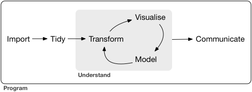
A typical data science project:
## [Tidyverse](https://www.tidyverse.org)
- `tidyverse` is a collection of R packages that make data wrangling easy.
- Install `tidyverse` from RStudio menu `Tools -> Install Packages...` or
```{r, eval = FALSE}
install.packages("tidyverse")
```
- After installation, load `tidyverse` by
```{r}
library("tidyverse")
```
# Tibble | r4ds chapter 10
## Tibbles
- Tibbles extend data frames in R and form the core of tidyverse.
## Create tibbles
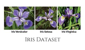
- `iris` is a dataframe available in base R:
```{r}
# a regular data frame
iris
```
- Convert a regular data frame to tibble:
```{r}
as_tibble(iris)
```
We see by default tibble only displays the first 10 rows of data.
- Convert a tibble to data frame:
```{r, eval = FALSE}
as.data.frame(tb)
```
----
- Create tibble from individual vectors. Note values for y are recycled:
```{r}
tibble(
x = 1:5,
y = 1,
z = x ^ 2 + y
)
```
----
- Transposed tibbles:
```{r}
tribble(
~x, ~y, ~z,
#--|--|----
"a", 2, 3.6,
"b", 1, 8.5
)
```
## Printing of a tibble
- By default, tibble prints the first 10 rows and all columns that fit on screen.
```{r}
nycflights13::flights
```
----
- To change number of rows and columns to display:
```{r}
nycflights13::flights %>%
print(n = 10, width = Inf)
```
Here we see the **pipe operator** `%>%` pipes the output from previous command to the (first) agument of the next command.
----
- To change the default print setting:
- `options(tibble.print_max = n, tibble.print_min = m)`: if more than `m` rows, print only `n` rows.
- `options(dplyr.print_min = Inf)`: print all row.
- `options(tibble.width = Inf)`: print all columns.
## Subsetting
-
```{r}
df <- tibble(
x = runif(5),
y = rnorm(5)
)
df
```
- Extract by name:
```{r}
df$x
df[["x"]]
```
----
- Extract by position:
```{r}
df[[1]]
```
- Pipe:
```{r}
df %>% .$x
df %>% .[["x"]]
```
# Data import | r4ds chapter 11
## readr
- readr package implements functions that turn flat files into tibbles.
- `read_csv()`, `read_csv2()` (semicolon seperated files), `read_tsv()`, `read_delim()`.
- `read_fwf()` (fixed width files), `read_table()`.
- `read_log()` (Apache style log files).
- An example file [heights.csv](https://raw.githubusercontent.com/ucla-biostat203b-2021winter/ucla-biostat203b-2021winter.github.io/master/slides/05-tidy/heights.csv):
```{bash}
head heights.csv
```
----
- Read from a local file [heights.csv](https://raw.githubusercontent.com/ucla-biostat203b-2021winter/ucla-biostat203b-2021winter.github.io/master/slides/05-tidy/heights.csv):
```{r}
heights <- read_csv("heights.csv")
heights
```
----
- I'm curious about relation between `earn` and `height` and `sex`
```{r}
ggplot(data = heights) +
geom_point(mapping = aes(x = height, y = earn, color = sex))
```
----
- Read from inline csv file:
```{r}
read_csv("a,b,c
1,2,3
4,5,6")
```
- Skip first `n` lines:
```{r}
read_csv("The first line of metadata
The second line of metadata
x,y,z
1,2,3", skip = 2)
```
----
- Skip comment lines:
```{r}
read_csv("# A comment I want to skip
x,y,z
1,2,3", comment = "#")
```
- No header line:
```{r}
read_csv("1,2,3\n4,5,6", col_names = FALSE)
```
----
- No header line and specify colnames:
```{r}
read_csv("1,2,3\n4,5,6", col_names = c("x", "y", "z"))
```
- Specify the symbol representing missing values:
```{r}
read_csv("a,b,c\n1,2,.", na = ".")
```
## Writing to a file
- Write to csv:
```{r, eval = FALSE}
write_csv(challenge, "challenge.csv")
```
- Write (and read) RDS files:
```{r, eval = FALSE}
write_rds(challenge, "challenge.rds")
read_rds("challenge.rds")
```
## Excel files
- readxl package (part of tidyverse) reads both xls and xlsx files:
```{r}
library(readxl)
# xls file
read_excel("datasets.xls")
```
```{r}
# xlsx file
read_excel("datasets.xlsx")
```
- List the sheet name:
```{r}
excel_sheets("datasets.xlsx")
```
- Read in a specific sheet by name or number:
```{r}
read_excel("datasets.xlsx", sheet = "mtcars")
```
```{r}
read_excel("datasets.xlsx", sheet = 4)
```
- Control subset of cells to read:
```{r}
# first 3 rows
read_excel("datasets.xlsx", n_max = 3)
```
Excel type range
```{r}
read_excel("datasets.xlsx", range = "C1:E4")
```
```{r}
# first 4 rows
read_excel("datasets.xlsx", range = cell_rows(1:4))
```
```{r}
# columns B-D
read_excel("datasets.xlsx", range = cell_cols("B:D"))
```
```{r}
# sheet
read_excel("datasets.xlsx", range = "mtcars!B1:D5")
```
- Specify `NA`s:
```{r}
read_excel("datasets.xlsx", na = "setosa")
```
- Writing Excel files: `openxlsx` and `writexl` packages.
## Other types of data
- **haven** reads SPSS, Stata, and SAS files.
- **DBI**, along with a database specific backend (e.g. **RMySQL**, **RSQLite**, **RPostgreSQL** etc) allows us to run SQL queries against a database and return a data frame. Later we will use DBI to work with databases.
- **jsonlite** reads json files.
- **xml2** reads XML files.
- **tidyxl** reads non-tabular data from Excel.
# Tidy data | r4ds chapter 12
## Tidy data
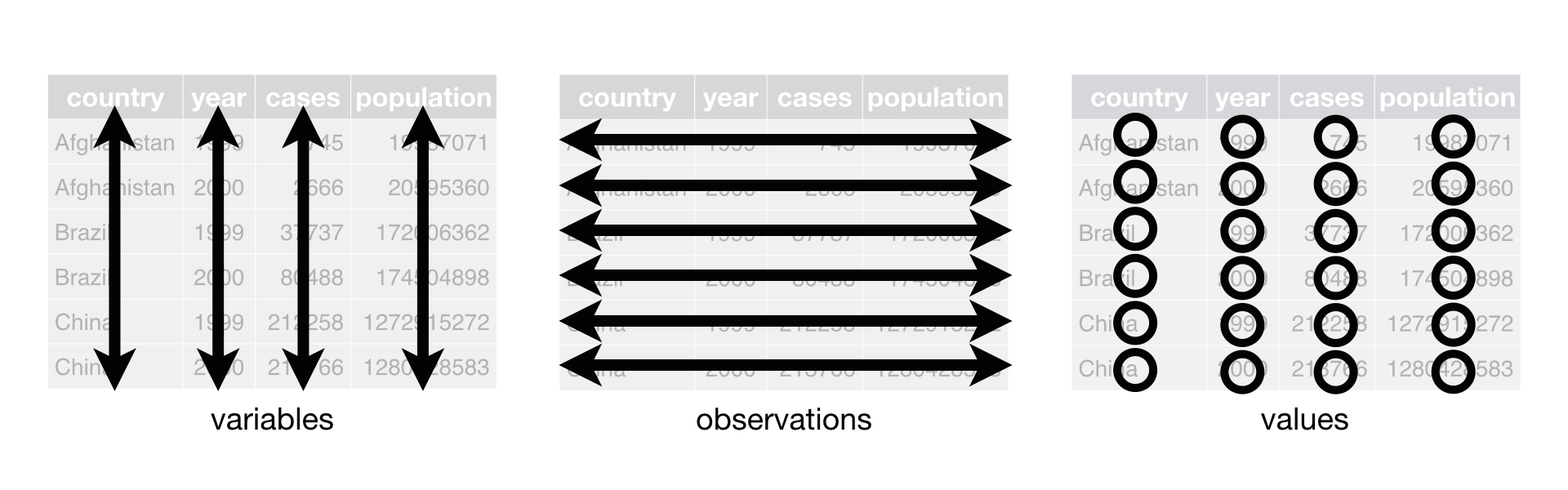
There are three interrelated rules which make a dataset tidy:
- Each variable must have its own column.
- Each observation must have its own row.
- Each value must have its own cell.
----
- Example table1
```{r}
table1
```
is tidy.
----
- Example table2
```{r}
table2
```
is not tidy.
----
- Example table3
```{r}
table3
```
is not tidy.
----
- Example table4a
```{r}
table4a
```
is not tidy.
- Example table4b
```{r}
table4b
```
is not tidy.
## Gathering (pivot_longer)
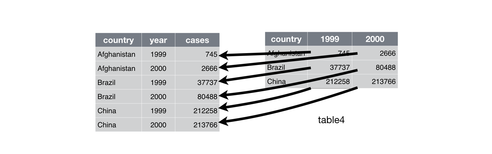
- `gather` columns into a new pair of variables.
```{r}
table4a %>%
gather(`1999`, `2000`, key = "year", value = "cases")
```
- `gather` function has been superseded by `pivot_longer`
```{r}
table4a %>%
pivot_longer(c(`1999`, `2000`), names_to = "year", values_to = "cases")
```
----
- We can gather table4b too and then join them
```{r}
tidy4a <- table4a %>%
pivot_longer(c(`1999`, `2000`), names_to = "year", values_to = "cases")
# gather(`1999`, `2000`, key = "year", value = "cases")
tidy4b <- table4b %>%
pivot_longer(c(`1999`, `2000`), names_to = "year", values_to = "population")
# gather(`1999`, `2000`, key = "year", value = "population")
left_join(tidy4a, tidy4b)
```
## Spreading
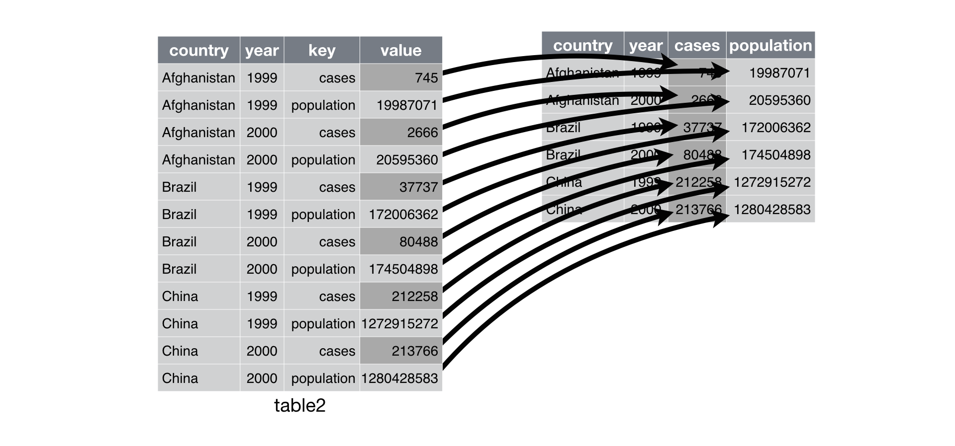
- Spreading is the opposite of gathering.
```{r}
table2 %>%
spread(key = type, value = count)
```
- `spread` function has been superseded by `pivot_wider`
```{r}
table2 %>%
pivot_wider(names_from = type, values_from = count)
```
## Separating
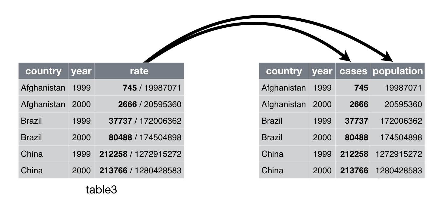
-
```{r}
table3 %>%
separate(rate, into = c("cases", "population"))
```
----
- Seperate into numeric values:
```{r}
table3 %>%
separate(rate, into = c("cases", "population"), convert = TRUE)
```
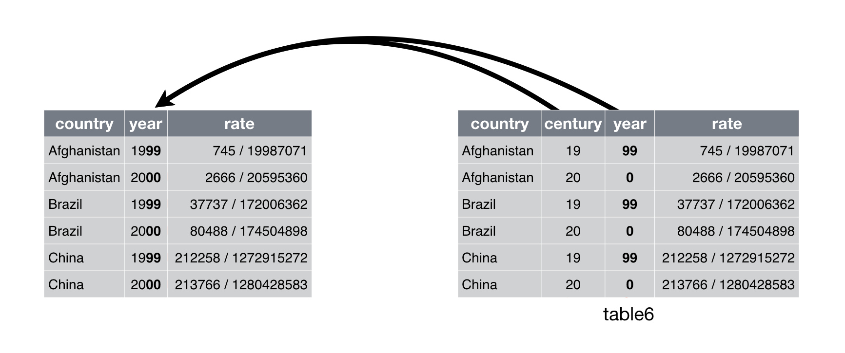
----
- Separate at a fixed position:
```{r}
table3 %>%
separate(year, into = c("century", "year"), sep = 2)
```
## Unite
-
```{r}
table5
```
----
- `unite()` is the inverse of `separate()`.
```{r}
table5 %>%
unite(new, century, year, sep = "")
```