---
title: "Data Transformation With dplyr"
author: "Dr. Hua Zhou @ UCLA"
date: "Jan 25, 2022"
subtitle: Biostat 203B
output:
# ioslides_presentation: default
html_document:
toc: true
toc_depth: 4
---
```{r setup, include=FALSE}
knitr::opts_chunk$set(fig.align = 'center', cache = TRUE)
```
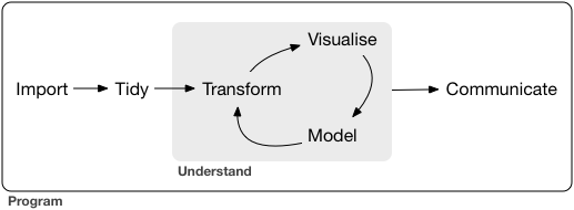
A typical data science project:
## nycflights13 data
- Available from the nycflights13 package.
- 336,776 flights that departed from New York City in 2013:
```{r}
library("tidyverse")
```
```{r}
library("nycflights13")
flights
```
- To display more rows:
```{r}
flights %>% print(n = 20)
```
Note `%>%` is the pipe in tidyverse. Above command is equivalent to `print(flights, n = 20)`.
- To display all rows:
```{r, eval = FALSE}
flights %>% print(n = nrow(.))
```
Do **not** try this on the `flights` data, which has too many rows.
- To display more columns (variables):
```{r}
flights %>% print(width = Inf)
```
The `width` argument controls the screen width.
## dplyr basics
* Pick observations (rows) by their values: `filter()`.
* Reorder the rows: `arrange()`.
* Pick variables (columns) by their names: `select()`.
* Create new variables with functions of existing variables: `mutate()`.
* Collapse many values down to a single summary: `summarise()`.
# Manipulate rows (cases)
## Filter rows with `filter()`
- Flights on Jan 1st:
```{r}
# same as filter(flights, month == 1 & day == 1)
filter(flights, month == 1, day == 1)
```
----
- Flights in Nov or Dec:
```{r}
filter(flights, month == 11 | month == 12)
```
## Remove rows with duplicate values
- One row from each month:
```{r}
distinct(flights, month, .keep_all = TRUE)
```
- With `.keep_all = FALSE`, only distinct values of the variable are selected:
```{r}
distinct(flights, month)
```
## Sample rows
- Randomly select `n` rows:
```{r}
sample_n(flights, 10, replace = TRUE)
```
----
- Randomly select fraction of rows:
```{r}
sample_frac(flights, 0.1, replace = TRUE)
```
## Select rows by position
- Select rows by position:
```{r}
slice(flights, 1:5)
```
- First rows:
```{r}
slice_head(flights, n = 5)
```
- Last rows:
```{r}
slice_tail(flights, n = 5)
```
----
- Top `n` rows with the highest values:
```{r}
# deprecated: top_n(flights, 5, wt = time_hour)
# This function is quick
slice_max(flights, n = 5, order_by = time_hour)
```
- Bottom `n` rows with lowest values:
```{r, eval=F}
# deprecated: top_n(flights, -5, wt = time_hour)
# Why it takes REALLY long???
# slice_max(flights, n = 5, order_by = desc(time_hour)) # is fast
slice_min(flights, n = 5, order_by = time_hour)
```
----
- `slice_*` verbs apply to groups for grouped tibbles.
## Arrange rows with `arrange()`
- Sort in ascending order:
```{r}
arrange(flights, year, month, day)
```
----
- Sort in descending order:
```{r}
arrange(flights, desc(arr_delay)) %>%
print(width = Inf)
```
----
- By default, `arrange` ignores grouping in grouped tibbles. Set `.by_group = TRUE` to arrange within each group.
# Manipulate columns (variables)
## Select columns with `select()`
- Select columns by variable names:
```{r}
select(flights, year, month, day)
```
- Pull values of _one_ column as a vector:
```{r, eval = FALSE}
pull(flights, year)
```
----
- Select columns between two variables:
```{r}
select(flights, year:day)
```
----
- Select columns _except_ those between two variables:
```{r, }
select(flights, -(year:day))
```
----
- Select columns by positions:
```{r}
select(flights, seq(1, 10, by = 2))
```
----
- Move variables to the start of data frame:
```{r}
select(flights, time_hour, air_time, everything())
```
----
- Helper functions.
* `starts_with("abc")`: matches names that begin with “abc”.
* `ends_with("xyz")`: matches names that end with “xyz”.
* `contains("ijk")`: matches names that contain “ijk”.
* `matches("(.)\\1")`: selects variables that match a regular expression.
* `num_range("x", 1:3)`: matches x1, x2 and x3.
* `one_of()`
## Add new variables with `mutate()`
- Add variables `gain` and `speed`:
```{r}
flights_sml <-
select(flights, year:day, ends_with("delay"), distance, air_time)
flights_sml
```
```{r}
mutate(flights_sml,
gain = arr_delay - dep_delay,
speed = distance / air_time * 60
)
```
----
- Refer to columns that you’ve just created:
```{r}
mutate(flights_sml,
gain = arr_delay - dep_delay,
hours = air_time / 60,
gain_per_hour = gain / hours
)
```
----
- Only keep the new variables by `transmute()`:
```{r}
transmute(flights,
gain = arr_delay - dep_delay,
hours = air_time / 60,
gain_per_hour = gain / hours
)
```
----
- `mutate_all()`: apply funs to all columns.
```{r, eval = FALSE}
mutate_all(data, funs(log(.), log2(.)))
```
- `mutate_at()`: apply funs to specific columns.
```{r, eval = FALSE}
mutate_at(data, vars(-Species), funs(log(.)))
```
- `mutate_if()`: apply funs of one type
```{r, eval = FALSE}
mutate_if(data, is.numeric, funs(log(.)))
```
# Summaries
## Summaries with `summarise()`
- Mean of a variable:
```{r}
summarise(flights, delay = mean(dep_delay, na.rm = TRUE))
```
----
- Convert a tibble into a grouped tibble:
```{r}
(by_day <- group_by(flights, year, month, day))
```
----
- Grouped summaries:
```{r}
summarise(by_day, delay = mean(dep_delay, na.rm = TRUE))
```
## Pipe
- Consider following analysis (find destinations excluding `HNL` that have >20 flights, and calculate the average distances and arrival delay):
```{r, message = FALSE}
by_dest <- group_by(flights, dest)
delay <- summarise(by_dest, count = n(),
dist = mean(distance, na.rm = TRUE),
delay = mean(arr_delay, na.rm = TRUE)
)
delay <- filter(delay, count > 20, dest != "HNL")
delay
```
----
- Cleaner code using pipe `%>%`:
```{r}
delays <- flights %>%
group_by(dest) %>%
summarise(
count = n(),
dist = mean(distance, na.rm = TRUE),
delay = mean(arr_delay, na.rm = TRUE)
) %>%
filter(count > 20, dest != "HNL")
delays
```
----
- ggplot2 accepts pipe too.
```{r}
delays %>%
ggplot(mapping = aes(x = dist, y = delay)) +
geom_point(aes(size = count), alpha = 1/3) +
geom_smooth(se = FALSE) +
labs(x = "Distance from NYC (miles)",
y = "Arrival delay (mins)")
```
## Other summary functions
- Location: `mean(x)`, `median(x)`.
```{r}
not_cancelled <- flights %>%
filter(!is.na(dep_delay), !is.na(arr_delay))
not_cancelled
```
```{r}
not_cancelled %>%
group_by(year, month, day) %>%
summarise(
avg_delay1 = mean(arr_delay),
avg_delay2 = mean(arr_delay[arr_delay > 0]) # the average positive delay
)
```
----
- Spread: `sd(x)`, `IQR(x)`, `mad(x)`.
```{r}
# destinations with largest variation in distance
not_cancelled %>%
group_by(dest) %>%
summarise(distance_sd = sd(distance)) %>%
arrange(desc(distance_sd))
```
----
- Rank: `min(x)`, `quantile(x, 0.25)`, `max(x)`.
```{r}
# Earliest and latest flights on each day?
not_cancelled %>%
group_by(year, month, day) %>%
summarise(
first = min(dep_time),
last = max(dep_time)
)
```
----
- Position: `first(x)`, `nth(x, 2)`, `last(x)`.
```{r}
not_cancelled %>%
group_by(year, month, day) %>%
summarise(
first_dep = first(dep_time),
last_dep = last(dep_time)
)
```
----
- Count: `n(x)`, `sum(!is.na(x))`, `n_distinct(x)`.
```{r}
# Which destinations have the most carriers?
not_cancelled %>%
group_by(dest) %>%
summarise(carriers = n_distinct(carrier)) %>%
arrange(desc(carriers))
```
----
-
```{r}
# which destination has most flights from NYC?
not_cancelled %>%
count(dest) %>%
arrange(desc(n))
```
----
-
```{r}
# which aircraft flew most in 2013?
not_cancelled %>%
count(tailnum, wt = distance) %>%
arrange(desc(n))
```
----
-
```{r}
# How many flights left before 5am? (these usually indicate delayed
# flights from the previous day)
not_cancelled %>%
group_by(year, month, day) %>%
summarise(n_early = sum(dep_time < 500)) %>%
arrange(desc(n_early))
```
----
-
```{r}
# What proportion of flights are delayed by more than an hour?
not_cancelled %>%
group_by(year, month, day) %>%
summarise(hour_perc = mean(arr_delay > 60)) %>%
arrange(desc(hour_perc))
```
## Grouped mutates (and filters)
- Recall the `flights_sml` tibble created earlier:
```{r}
flights_sml
```
- Find the worst members of each group:
```{r}
flights_sml %>%
group_by(year, month, day) %>%
filter(rank(desc(arr_delay)) < 10)
```
----
- Find all groups bigger than a threshold:
```{r}
(popular_dests <- flights %>%
group_by(dest) %>%
filter(n() > 365))
```
----
- Standardise to compute per group metrics:
```{r}
popular_dests %>%
filter(arr_delay > 0) %>%
mutate(prop_delay = arr_delay / sum(arr_delay)) %>%
select(year:day, dest, arr_delay, prop_delay) %>%
print(width = Inf)
```
# Combine tables
nycflights13 package has >1 tables:
- We already know a lot about flights:
```{r}
flights %>% print(width = Inf)
```
----
- airlines:
```{r}
airlines
```
----
- airports:
```{r}
airports
```
----
- planes:
```{r}
planes
```
----
- Weather:
```{r}
weather %>%
print(width = Inf)
```
## Relational data
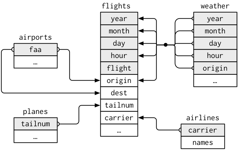
For the MIMIC-III data, the relation structure can be explored at .
## Keys
- A **primary key** uniquely identifies an observation in its own table.
- A **foreign key** uniquely identifies an observation in another table.
# Combine variables (columns)
## Demo tables
-
```{r}
(x <- tribble(
~key, ~val_x,
1, "x1",
2, "x2",
3, "x3"
))
```
```{r}
(y <- tribble(
~key, ~val_y,
1, "y1",
2, "y2",
4, "y3"
))
```
## Inner join
- An **inner join** matches pairs of observations whenever their keys are equal:
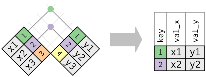
-
```{r}
inner_join(x, y, by = "key")
```
Same as
```{r, eval = FALSE}
x %>% inner_join(y, by = "key")
```
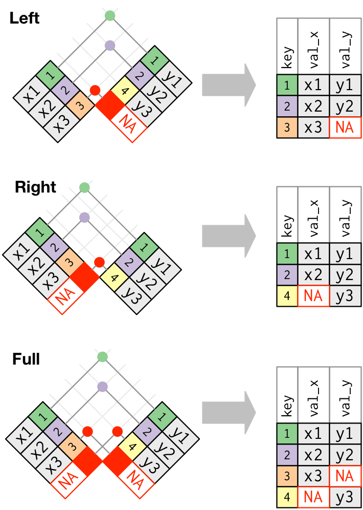
## Outer join
- An **outer join** keeps observations that appear in at least one of the tables.
- Three types of outer joins:
- A **left join** keeps all observations in `x`.
```{r}
left_join(x, y, by = "key")
```
- A **right join** keeps all observations in `y`.
```{r}
right_join(x, y, by = "key")
```
- A **full join** keeps all observations in `x` or `y`.
```{r}
full_join(x, y, by = "key")
```
## Duplicate keys
- One table has duplicate keys.
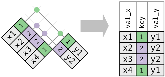
----
-
```{r}
x <- tribble(
~key, ~val_x,
1, "x1",
2, "x2",
2, "x3",
1, "x4"
)
y <- tribble(
~key, ~val_y,
1, "y1",
2, "y2"
)
left_join(x, y, by = "key")
```
----
- Both tables have duplicate keys. You get all possible combinations, the Cartesian product:
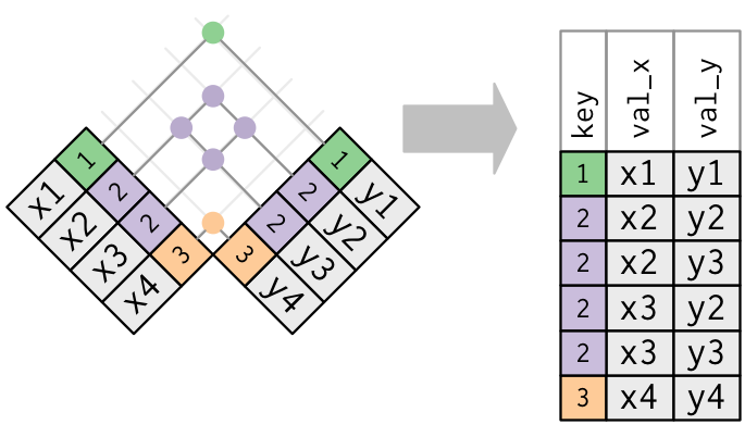
----
-
```{r}
x <- tribble(
~key, ~val_x,
1, "x1",
2, "x2",
2, "x3",
3, "x4"
)
y <- tribble(
~key, ~val_y,
1, "y1",
2, "y2",
2, "y3",
3, "y4"
)
left_join(x, y, by = "key")
```
----
- Let's create a narrower table from the flights data:
```{r}
flights2 <- flights %>%
select(year:day, hour, origin, dest, tailnum, carrier)
flights2
```
- We want to merge with the `weather` table:
```{r}
weather
```
## Defining the key columns
- `by = NULL` (default): use all variables that appear in both tables:
```{r}
# same as: flights2 %>% left_join(weather)
left_join(flights2, weather)
```
----
- `by = "x"`: use the common variable `x`:
```{r}
# same as: flights2 %>% left_join(weather)
left_join(flights2, planes, by = "tailnum")
```
----
- `by = c("a" = "b")`: match variable `a` in table `x` to the variable `b` in table `y`.
```{r}
# same as: flights2 %>% left_join(weather)
left_join(flights2, airports, by = c("dest" = "faa"))
```
# Combine cases (rows)
----
- Top 10 most popular destinations:
```{r}
top_dest <- flights %>%
count(dest, sort = TRUE) %>%
head(10)
top_dest
```
- How to filter the cases that fly to these destinations?
## Semi-join
- `semi_join(x, y)` keesp the rows in `x` that have a match in `y`.
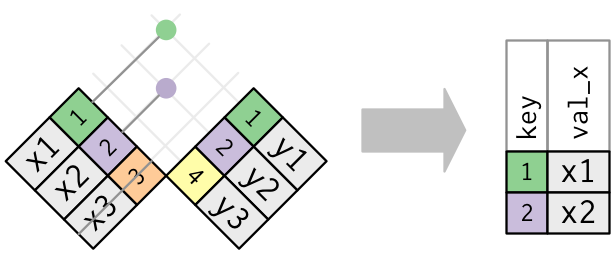
----
-
```{r}
semi_join(flights, top_dest)
```
## Anti-join
- `anti_join(x, y)` keeps the rows that don’t have a match.
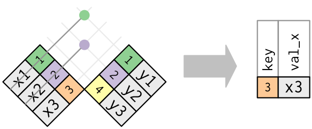
- Useful to see what will not be joined.
----
-
```{r}
flights %>%
anti_join(planes, by = "tailnum") %>%
count(tailnum, sort = TRUE)
```
## Set operations
- Generate two tables:
```{r}
(df1 <- tribble(
~x, ~y,
1, 1,
2, 1
))
```
```{r}
(df2 <- tribble(
~x, ~y,
1, 1,
1, 2
))
```
----
- `bind_rows(x, y)` stacks table `x` one on top of `y`.
```{r}
bind_rows(df1, df2)
```
- `intersect(x, y)` returns rows that appear in both `x` and `y`.
```{r}
intersect(df1, df2)
```
----
- `union(x, y)` returns unique observations in `x` and `y`.
```{r}
union(df1, df2)
```
----
- `setdiff(x, y)` returns rows that appear in `x` but not in `y`.
```{r}
setdiff(df1, df2)
```
```{r}
setdiff(df2, df1)
```
# Cheat sheet
[RStudio cheat sheet](https://raw.githubusercontent.com/rstudio/cheatsheets/master/data-transformation.pdf) is extremely helpful.