{width=500px}
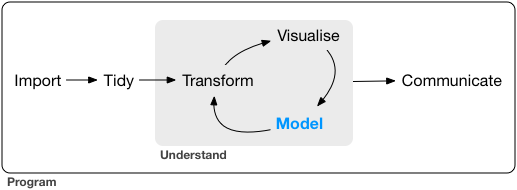
In the next two lectures, we discuss a general framework for learning, neural networks. ## History and recent surge From [Wang and Raj (2017)](https://arxiv.org/pdf/1702.07800.pdf):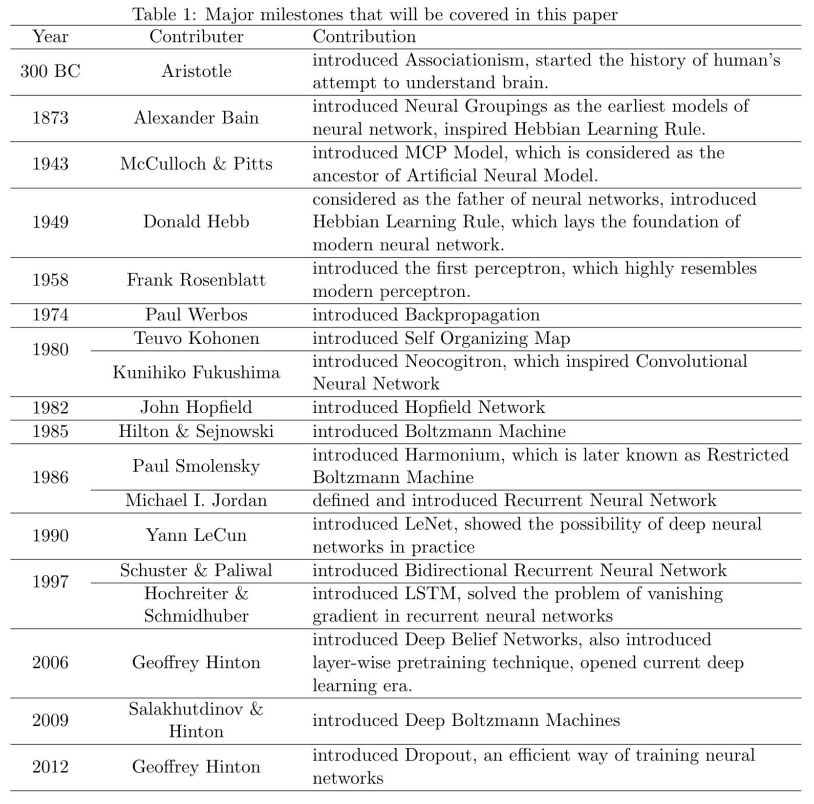{width=500px}
The current AI wave came in 2012 when AlexNet (60 million parameters) cuts the error rate of ImageNet competition (classify 1.2 million natural images) by half.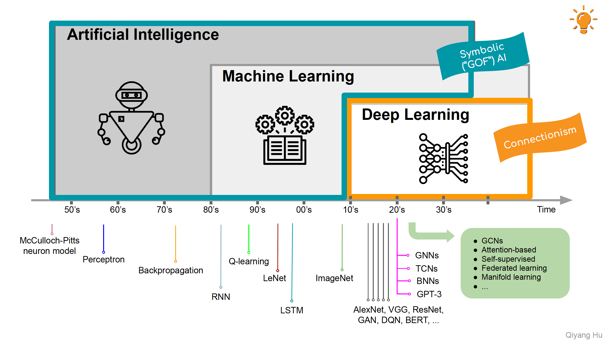{width=750px}
## Learning sources This lecture draws heavily on following sources. - _Elements of Statistical Learning_ (ESL) Chapter 11: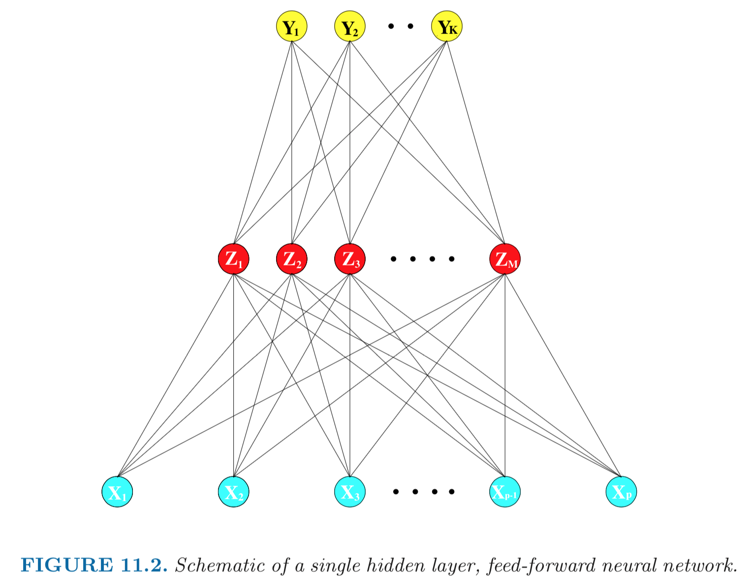{width=500px}
- Inspired by the biological neuron model.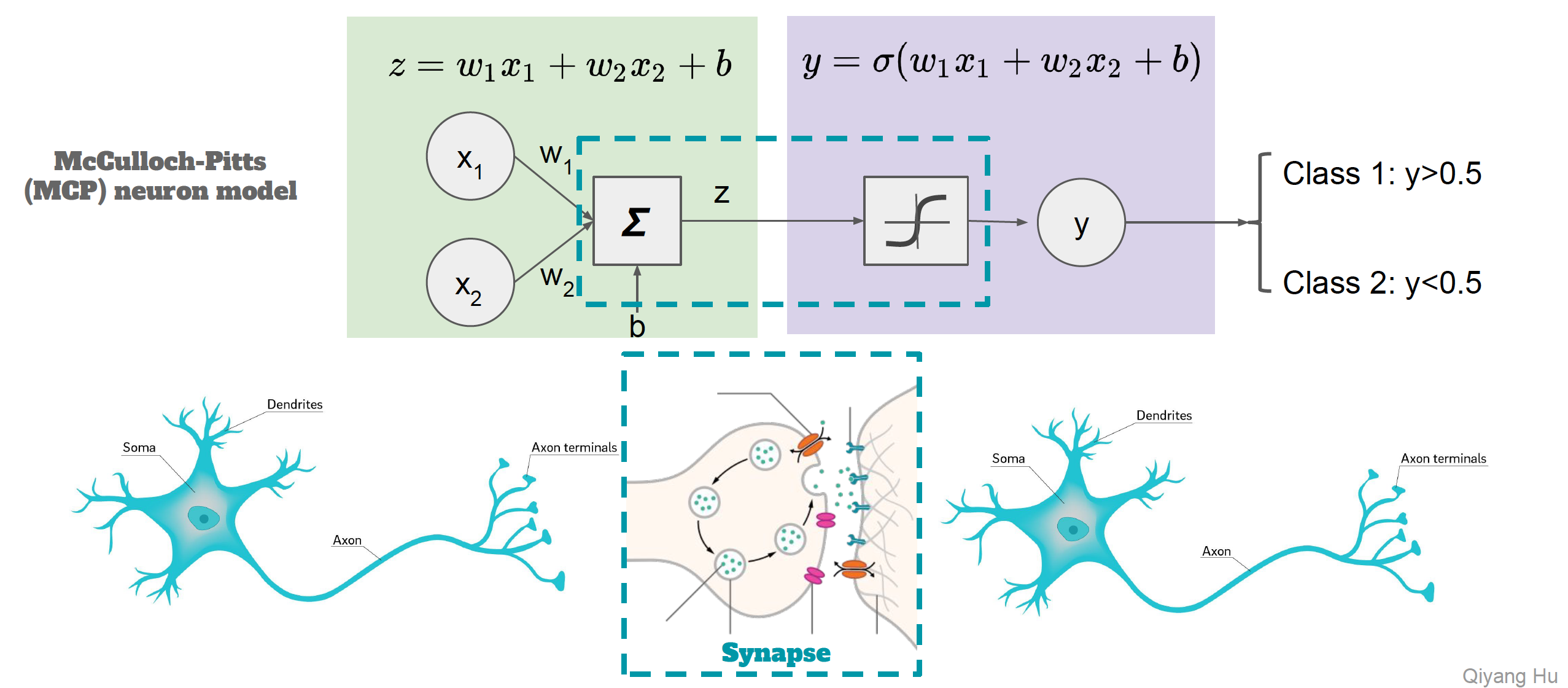{width=500px}
- Mathematical model: \begin{eqnarray*} Z_m &=& \sigma(\alpha_{0m} + \alpha_m^T X), \quad m = 1, \ldots, M \\ T_k &=& \beta_{0k} + \beta_k^T Z, \quad k = 1,\ldots, K \\ Y_k &=& f_k(X) = g_k(T), \quad k = 1, \ldots, K. \end{eqnarray*} - **Output layer**: $Y=(Y_1, \ldots, Y_K)$ are $K$-dimensional output. For univariate response, $K=1$; for $K$-class classification, $k$-th unit models the probability of class $k$. - **Input layer**: $X=(X_1, \ldots, X_p)$ are $p$-dimensional input features. - **Hidden layer**: $Z=(Z_1, \ldots, Z_M)$ are derived features created from linear combinations of inputs $X$. - $T=(T_1, \ldots, T_K)$ are the output features that are directly associated with the outputs $Y$ through output functions $g_k(\cdot)$. - $g_k(T) = T_k$ for regression. $g_k(T) = e^{T_k} / \sum_{k=1}^K e^{T_k}$ for $K$-class classification (**softmax regression**). - Number of **weights** (parameters) is $M(p+1) + K(M+1)$. - **Activation function** $\sigma$: - $\sigma(v)=$ a **step function**: human brain models where each unit represents a neuron, and the connections represent synapses; the neurons fired when the total signal passed to that unit exceeded a certain threshold. - **Sigmoid** function: $$ \sigma(v) = \frac{1}{1 + e^{-v}}. $$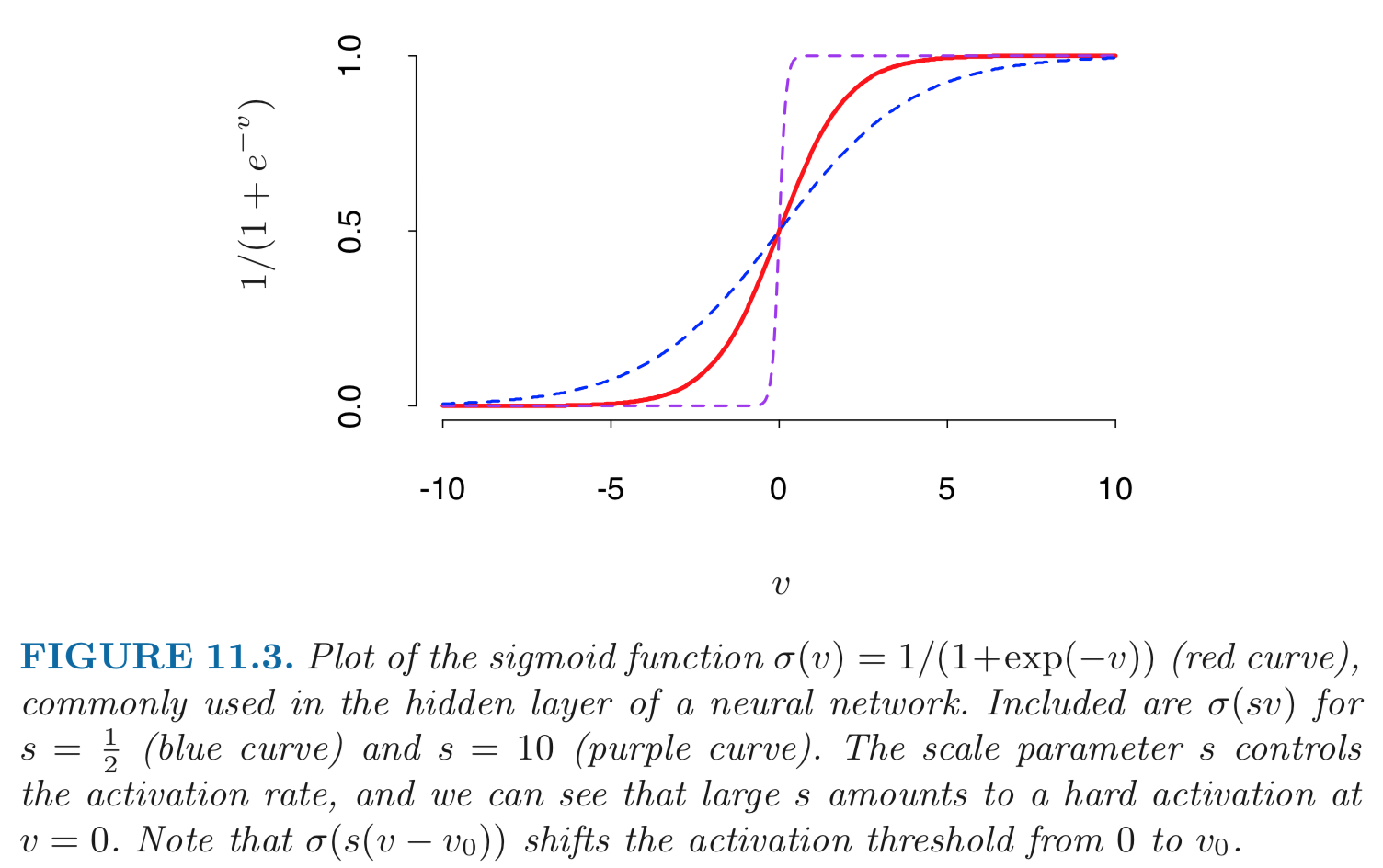{width=500px}
- **Rectifier**. $\sigma(v) = v_+ = \max(0, v)$. A unit employing the rectifier is called a **rectified linear unit (ReLU)**. According to Wikipedia: _The rectifier is, as of 2017, the most popular activation function for deep neural networks_. - **Softplus**. $\sigma(v) = \log (1 + \exp v)$.{width=400px}
- Given training data $(X_1, Y_1), \ldots, (X_n, Y_n)$, the **loss function** $L$ can be: - Sum of squares error (SSE): $$ L = \sum_{i=1}^n \sum_{k=1}^K [y_{ik} - f_k(x_i)]^2. $$ - Cross-entropy (deviance): $$ L = - \sum_{i=1}^n \sum_{k=1}^K y_{ik} \log f_k(x_i). $${width=400px}
[image source](https://towardsdatascience.com/https-medium-com-piotr-skalski92-deep-dive-into-deep-networks-math-17660bc376ba) - Model fitting: **back-propagation** (gradient descent) - Consider sum of squares error and let \begin{eqnarray*} z_{mi} &=& \sigma(\alpha_{0m} + \alpha_m^T x_i) \\ R_i &=& \sum_{k=1}^K [y_{ik} - f_k(x_i)]^2. \end{eqnarray*} - The derivatives: \begin{eqnarray*} \frac{\partial R_i}{\partial \beta_{km}} &=& -2 [y_{ik} - f_k(x_i)] g_k'(\beta_k^T z_i) z_{mi} \equiv \delta_{ki} z_{mi} \\ \frac{\partial R_i}{\partial \alpha_{ml}} &=& - 2 \sum_{k=1}^K [y_{ik} - f_k(x_i)] g_k'(\beta_k^T z_i) \beta_{km} \sigma'(\alpha_m^T x_i) x_{il} \equiv s_{mi} x_{il}. \end{eqnarray*} - Gradient descent update: \begin{eqnarray*} \beta_{km}^{(r+1)} &=& \beta_{km}^{(r)} - \gamma_r \sum_{i=1}^n \frac{\partial R_i}{\partial \beta_{km}} \\ \alpha_{ml}^{(r+1)} &=& \alpha_{ml}^{(r)} - \gamma_r \sum_{i=1}^n \frac{\partial R_i}{\partial \alpha_{ml}}, \end{eqnarray*} where $\gamma_r$ is the **learning rate**. - Back-propagation equations $$ s_{mi} = \sigma'(\alpha_m^T x_i) \sum_{k=1}^K \beta_{km} \delta_{ki}. $$ - Two-pass updates: \begin{eqnarray*} & & \text{initialization} \to \widehat{f}_k(x_i) \quad \quad \quad \text{(forward pass)} \\ &\to& \delta_{ki} \to s_{mi} \to \widehat{\beta}_{km} \text{ and } \widehat{\alpha}_{ml} \quad \quad \text{(backward pass)}. \end{eqnarray*} - Advantages: each hidden unit passes and receives information only to and from units that share a connection; can be implemented efficiently on a parallel architecture computer. - Stochastic gradient descent (**SGD**). In real machine learning applications, training set can be large. Back-propagation over all training cases can be expensive. Learning can also be carried out **online** — processing each batch one at a time, updating the gradient after each training batch, and cycling through the training cases many times. A training **epoch** refers to one sweep through the entire training set. **AdaGrad** and **RMSProp** improve the stability of SGD by trying to incorpoate Hessian information in a computationally cheap way. - Neural network model is a **projection pursuit** type additive model: $$ f(X) = \beta_0 + \sum_{m=1}^M \beta_m \sigma(\alpha_{m0} + \alpha_M^T X). $$ ## Multi-layer neural network (MLP) - Aka multi-layer perceptron (MLP). - 1 hidden layer: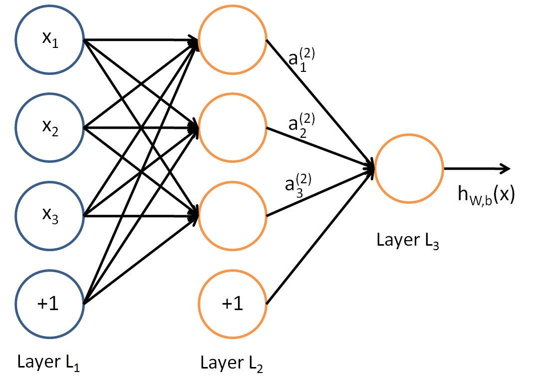{width=400px}
- 2 hidden layers:{width=400px}
## Expressivity of neural network - Playground: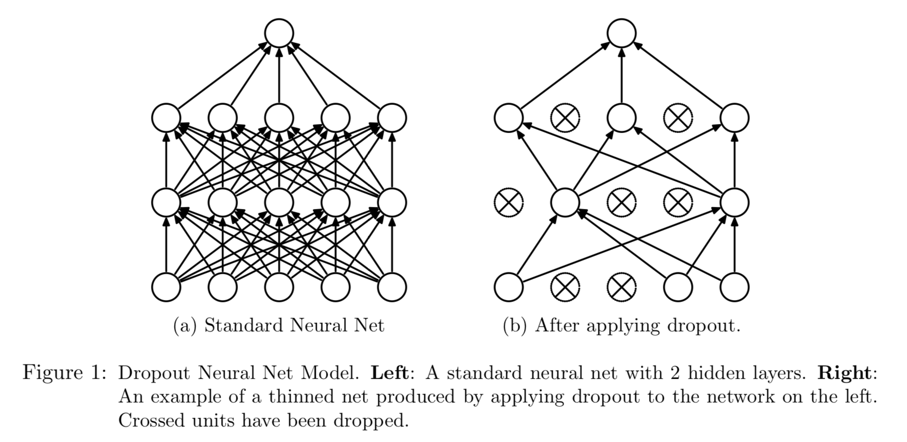{width=500px}
Figure from [Srivastava, Hinton, Krizhevsky, Sutskever, and Salakhutdinov (2014)](https://www.cs.toronto.edu/~hinton/absps/JMLRdropout.pdf). - How many hidden units and how many hidden layers: guided by domain knowledge and experimentation. - Multiple minima: try with different starting values. ## Convolutional neural networks (CNN) Sources: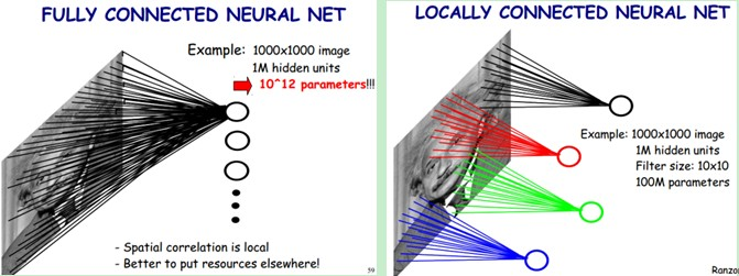{width=500px}
- **Fully connected networks** don't scale well with dimension of input images. E.g. $1000 \times 1000$ images have about $10^6$ input units, and assuming you want to learn 1 million features (hidden units), you have about $10^{12}$ parameters to learn! - In **locally connected networks**, each hidden unit only connects to a small contiguous region of pixels in the input, e.g., a patch of image or a time span of the input audio. - **Convolutions**. Natural images have the property of being **stationary**, meaning that the statistics of one part of the image are the same as any other part. This suggests that the features that we learn at one part of the image can also be applied to other parts of the image, and we can use the same features at all locations by **weight sharing**.{width=400px}
Consider $96 \times 96$ images. For each feature, first learn a $8 \times 8$ **feature detector** (or **filter** or **kernel**) from (possibly randomly sampled) $8 \times 8$ patches from the larger image. Then apply the learned detector to all $8 \times 8$ regions of the $96 \times 96$ image to obtain one $89 \times 89$ convolved feature for that feature. Interactive visualization: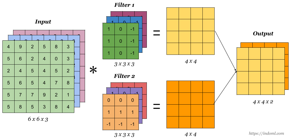{width=400px}
Source:{width=400px}
- **Convolutional neural network (CNN)**. Convolution + pooling + multi-layer neural networks. ## Popular datasets for computer vision tasks - [MNIST](http://yann.lecun.com/exdb/mnist/)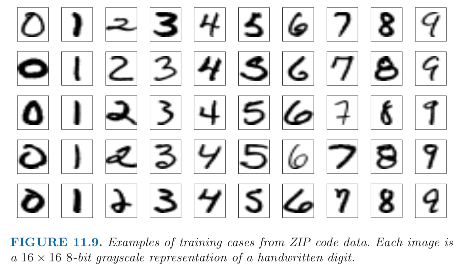{width=500px}
- [Fashion MNIST](https://github.com/zalandoresearch/fashion-mnist#fashion-mnist){width=500px}
- [CIFAR 10](https://www.cs.toronto.edu/~kriz/cifar.html)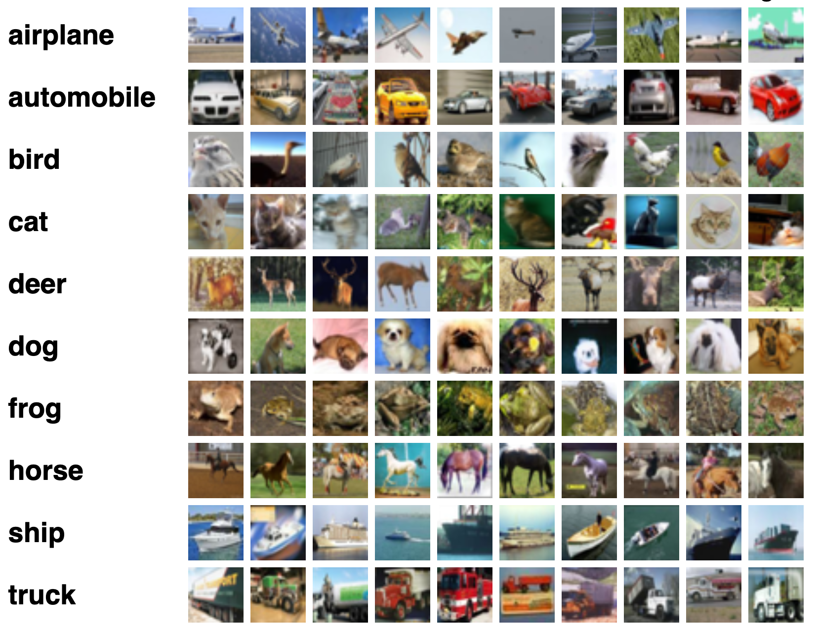{width=500px}
- [ImageNet](https://www.image-net.org/)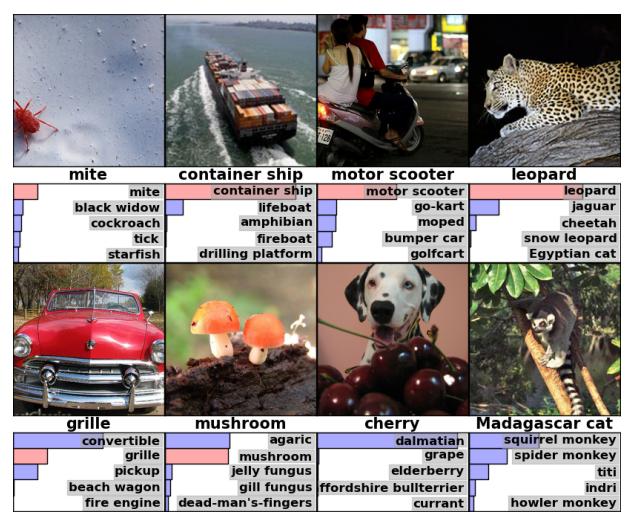{width=500px}
- [Microsoft COCO](https://cocodataset.org/#home) (object detection, segmentation, and captioning)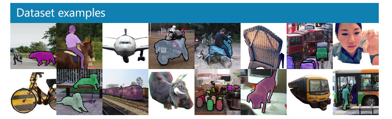{width=500px}
- [ADE20K](http://groups.csail.mit.edu/vision/datasets/ADE20K/) (scene parsing)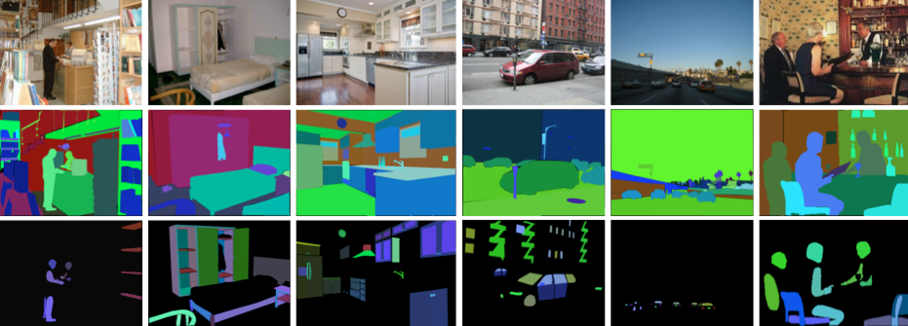{width=500px}
## Example: MNIST and LeNet-5{width=500px}
- Input: 256 pixel values from $16 \times 16$ grayscale images. Output: 0, 1, ..., 9, 10 class-classification. - On **MNIST** (60,000 training images, 10,000 testing images), accuracies of following methods were reported: | Method | Error rate | |--------|----------| | tangent distance with 1-nearest neighbor classifier | 1.1% | | degree-9 polynomial SVM | 0.8% | | LeNet-5 | 0.8% | | boosted LeNet-4 | 0.7% | - [LeNet-5](http://yann.lecun.com/exdb/publis/pdf/lecun-98.pdf) (1998) represents the state of the art in 1990s. $\sim 60$ thousand parameters.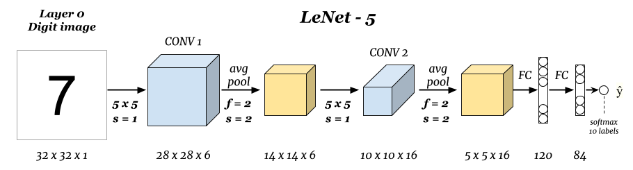{width=500px}
## Example: ImageNet and AlexNet Source: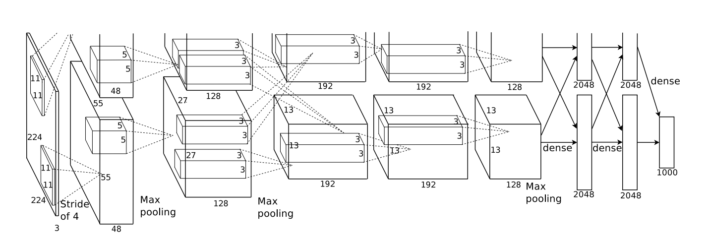{width=500px}
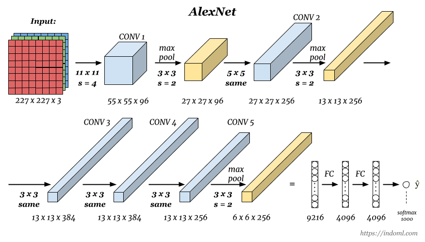{width=500px}
- AlexNet was the winner of the ImageNet Large Scale Visual Recognition Challenge (ILSVRC) classification the benchmark in 2012. - Achieved 62.5% accuracy:{width=500px}
96 learnt filters: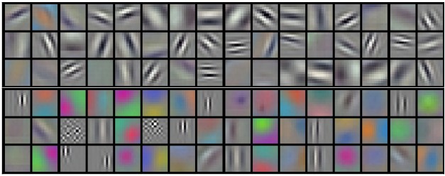{width=500px}
## Other popular architectures for image classification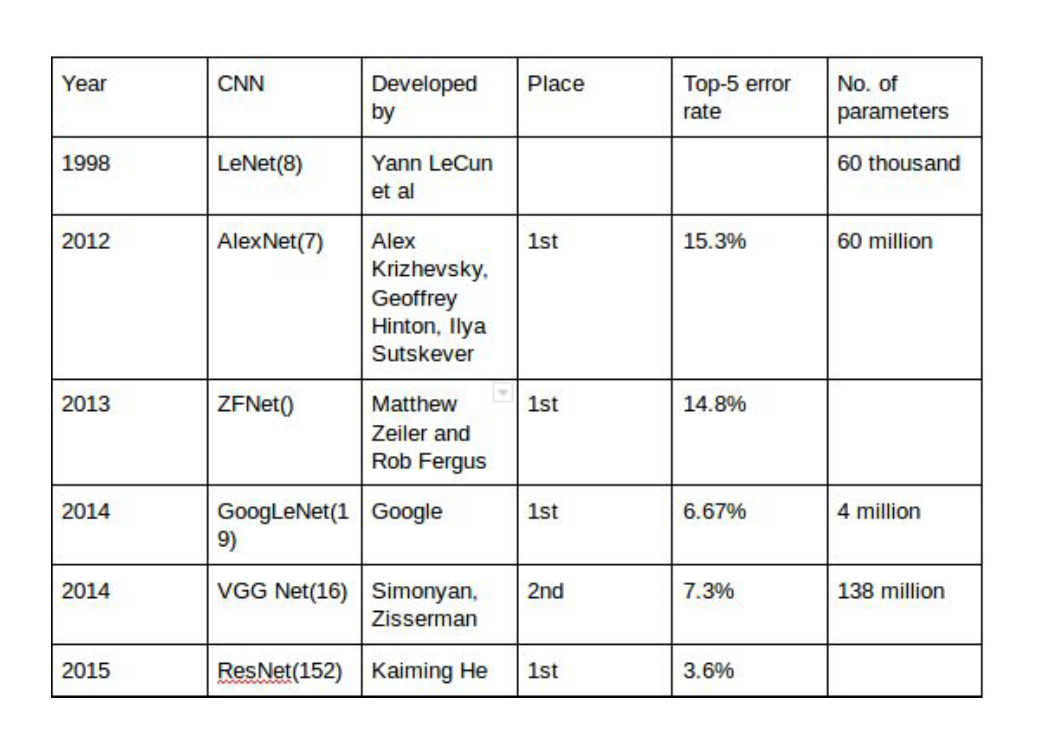{width=500px}
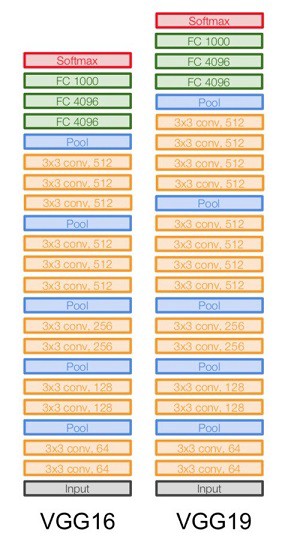
Source: [Architecture comparison of AlexNet, VGGNet, ResNet, Inception, DenseNet](https://towardsdatascience.com/architecture-comparison-of-alexnet-vggnet-resnet-inception-densenet-beb8b116866d) - [**VGG-16**](https://arxiv.org/abs/1409.1556) and VGG-19 (2014). The numbers 16 and 19 refer to the number of trainable layers. VGG-16 has $\sim 138$ million parameters. **VGGNet** was the runner up of the ImageNet Large Scale Visual Recognition Challenge (ILSVRC) classification the benchmark in 2014.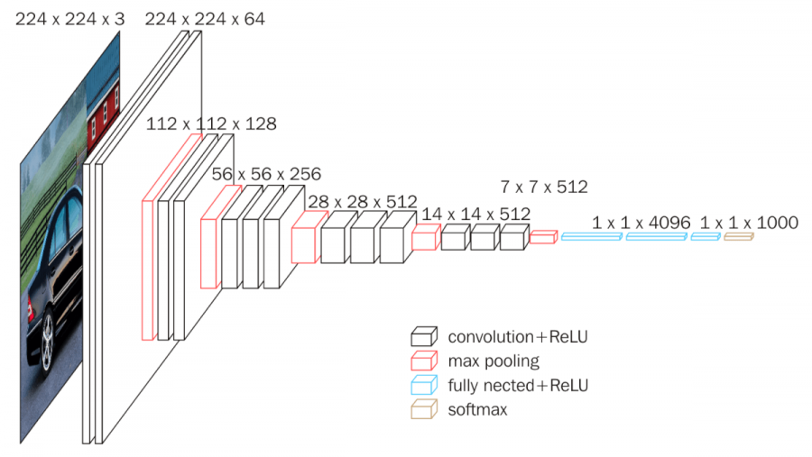{width=400px}
{height=400px}
{width=400px}
- [**ResNet**](https://arxiv.org/abs/1512.03385) secured 1st Position in ILSVRC and COCO 2015 competition with an error rate of 3.6% (Better than Human Performance !!!) Batch Normalization after every conv layer. It also uses Xavier initialization with SGD + Momentum. The learning rate is 0.1 and is divided by 10 as validation error becomes constant. Moreover, batch-size is 256 and weight decay is 1e-5. The important part is there is no dropout is used in ResNet.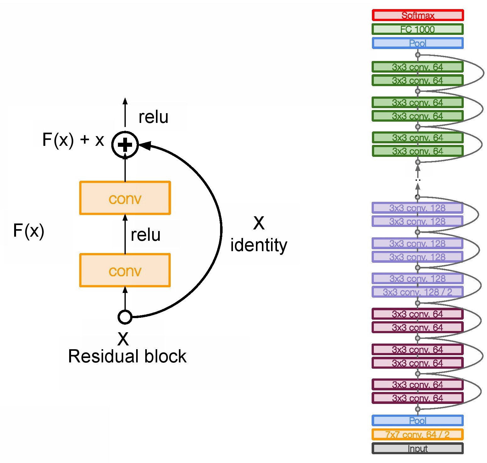{width=400px}
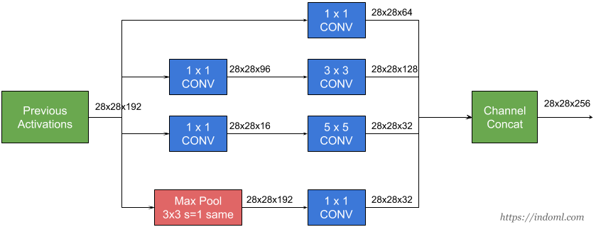
- **Inception**. Inception-v3 with 144 crops and 4 models ensembled, the top-5 error rate of 3.58% is obtained, and finally obtained 1st Runner Up (image classification) in ILSVRC 2015. The motivation of the inception network is, rather than requiring us to pick the filter size manually, let the network decide what is best to put in a layer. [GoogLeNet](https://arxiv.org/abs/1409.4842) has 9 inception modules.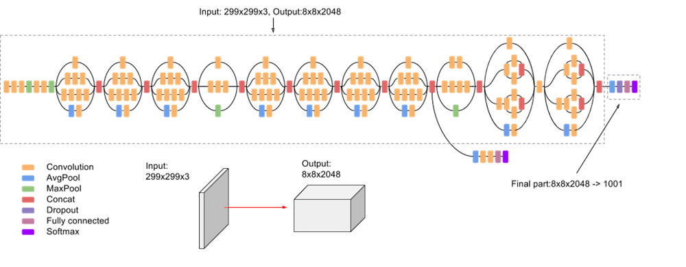{width=600px}
{width=500px}
## Recurrent neural networks (RNN) - Sources: -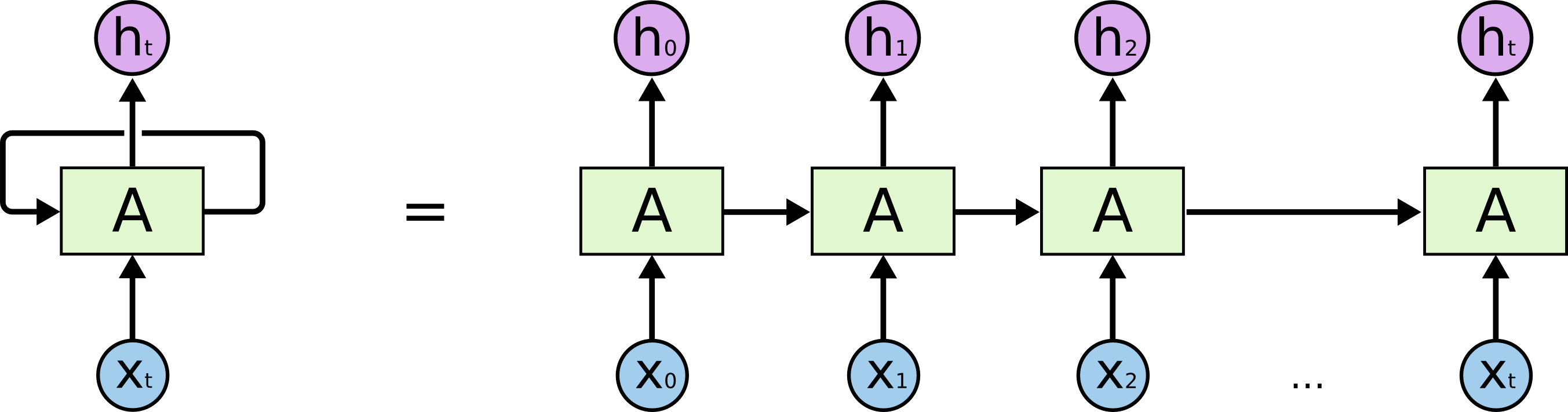{width=500px}
- RNNs allow us to operate over sequences of vectors: sequences in the input, the output, or in the most general case both. - Applications of RNN: - [Language modeling and generating text](http://karpathy.github.io/2015/05/21/rnn-effectiveness/). E.g., search prompt, messaging/email prompt, ...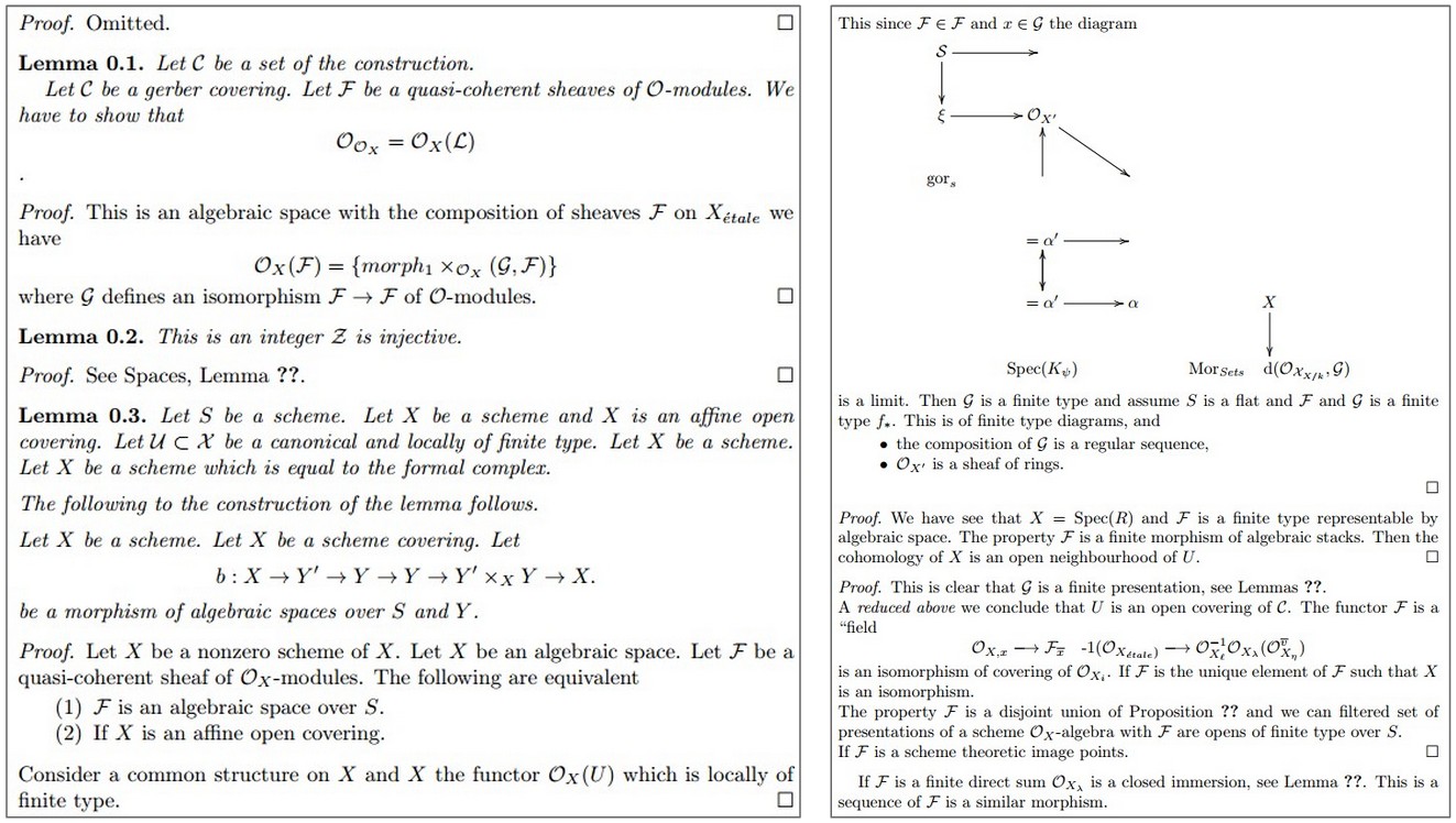{width=500px}
Above: generated (fake) LaTeX on algebraic geometry; see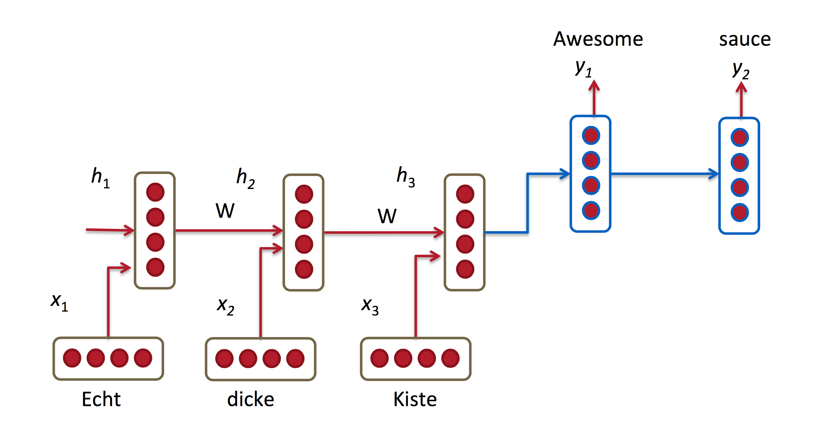{width=500px}
- **Computer vision**: image captioning, video captioning, ...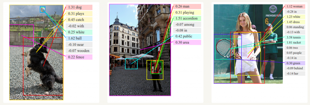{width=500px}
- RNNs accept an input vector $x$ and give you an output vector $y$. However, crucially this output vector’s contents are influenced not only by the input you just fed in, but also on the entire history of inputs you’ve fed in the past. - Short-term dependencies: to predict the last word in "the clouds are in the _sky_":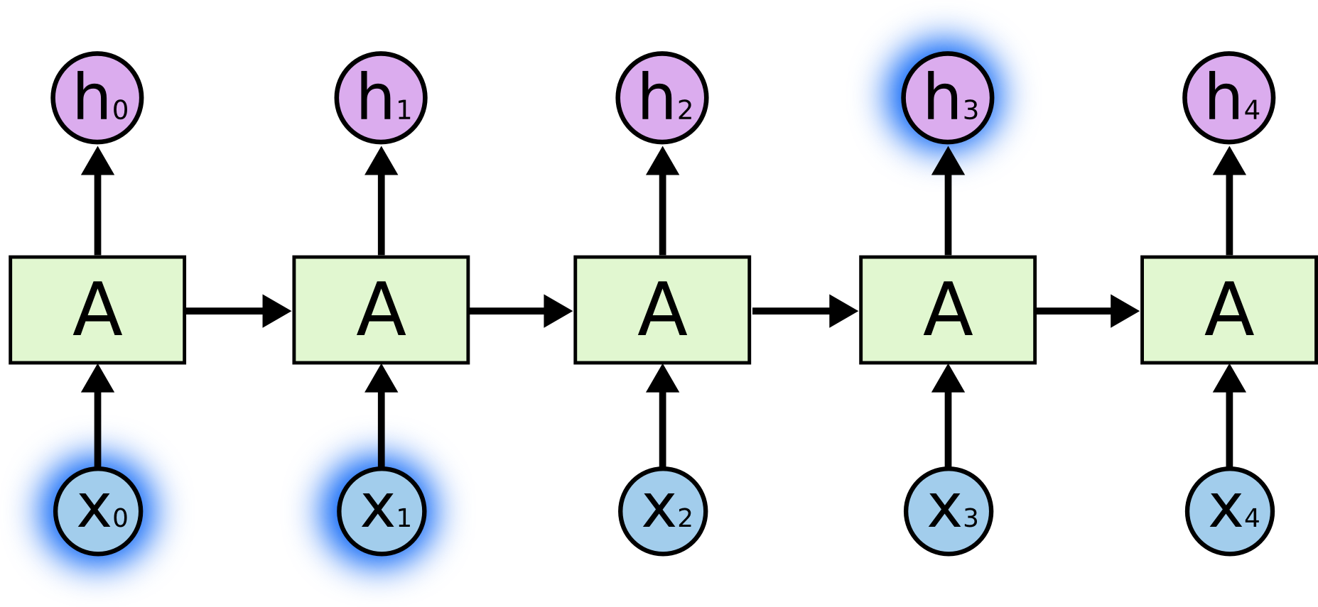{width=500px}
- Long-term dependencies: to predict the last word in "I grew up in France... I speek fluent _French_":{width=500px}
- Typical RNNs are having trouble with learning long-term dependencies.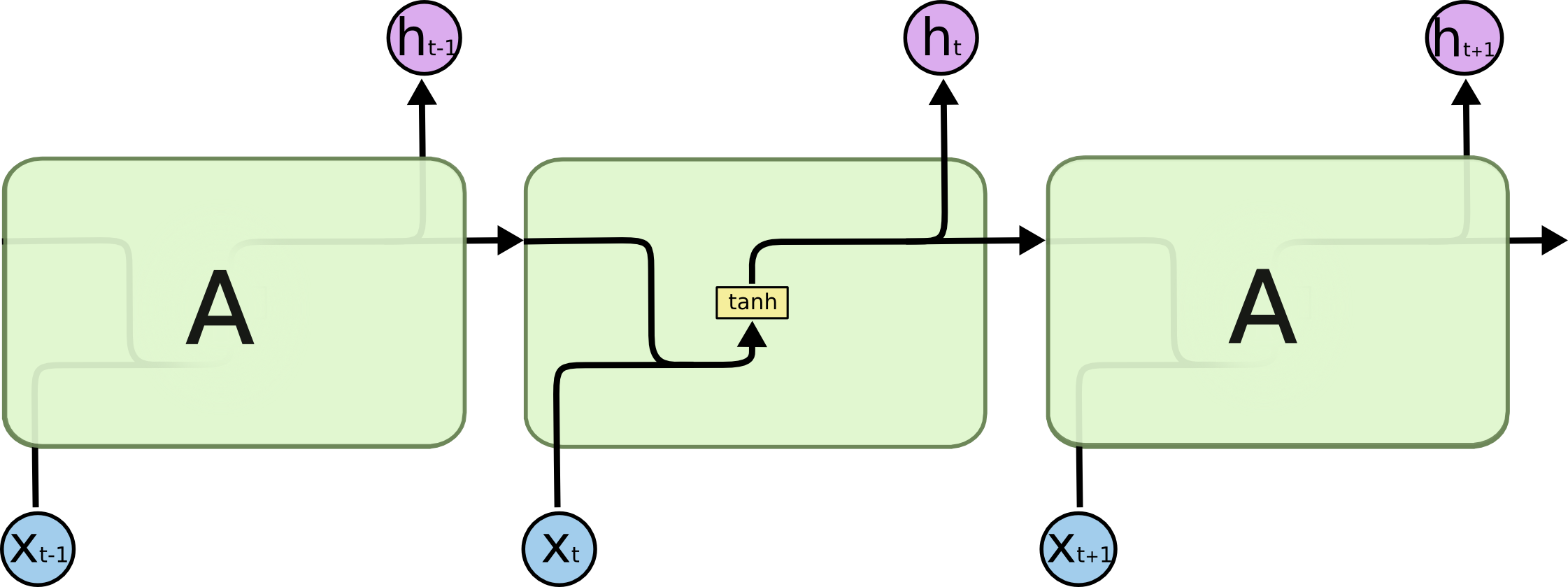{width=500px}
- **Long Short-Term Memory networks (LSTM)** are a special kind of RNN capable of learning long-term dependencies.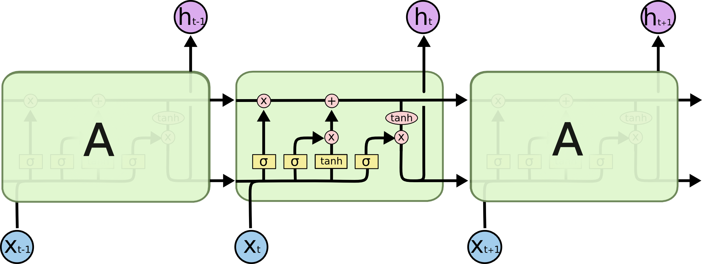{width=500px} 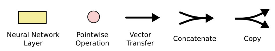{width=500px}
The **cell state** allows information to flow along it unchanged.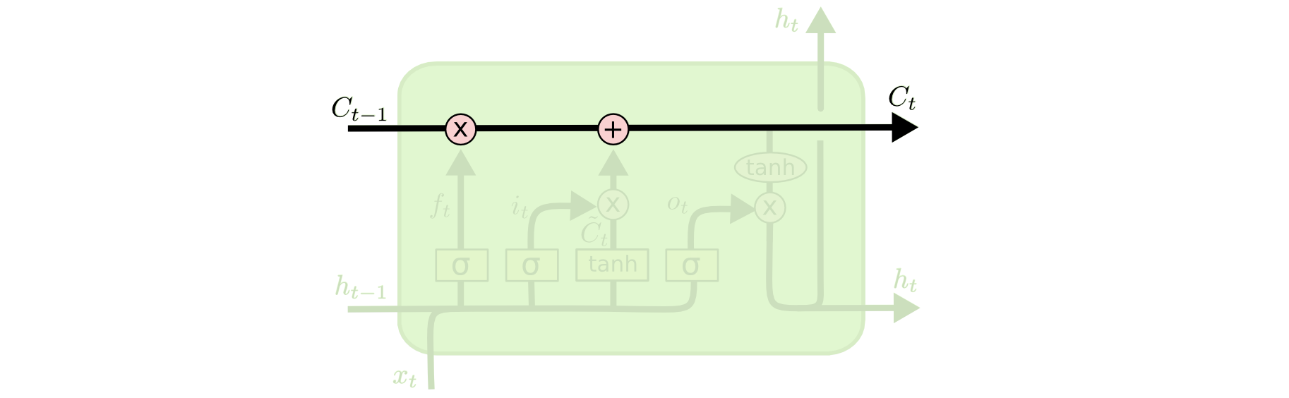{width=500px}
The **gates** give the ability to remove or add information to the cell state.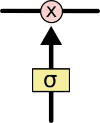{width=100px}
## Generative Adversarial Networks (GANs)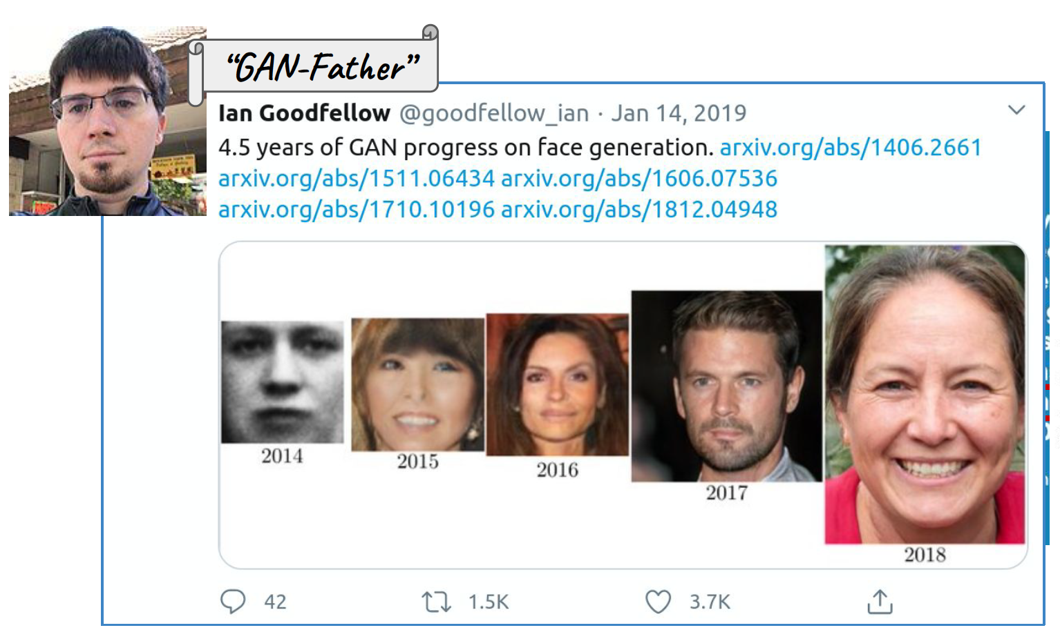{width=400px}
> The coolest idea in deep learning in the last 20 years. > - Yann LeCun on GANs. - Sources: -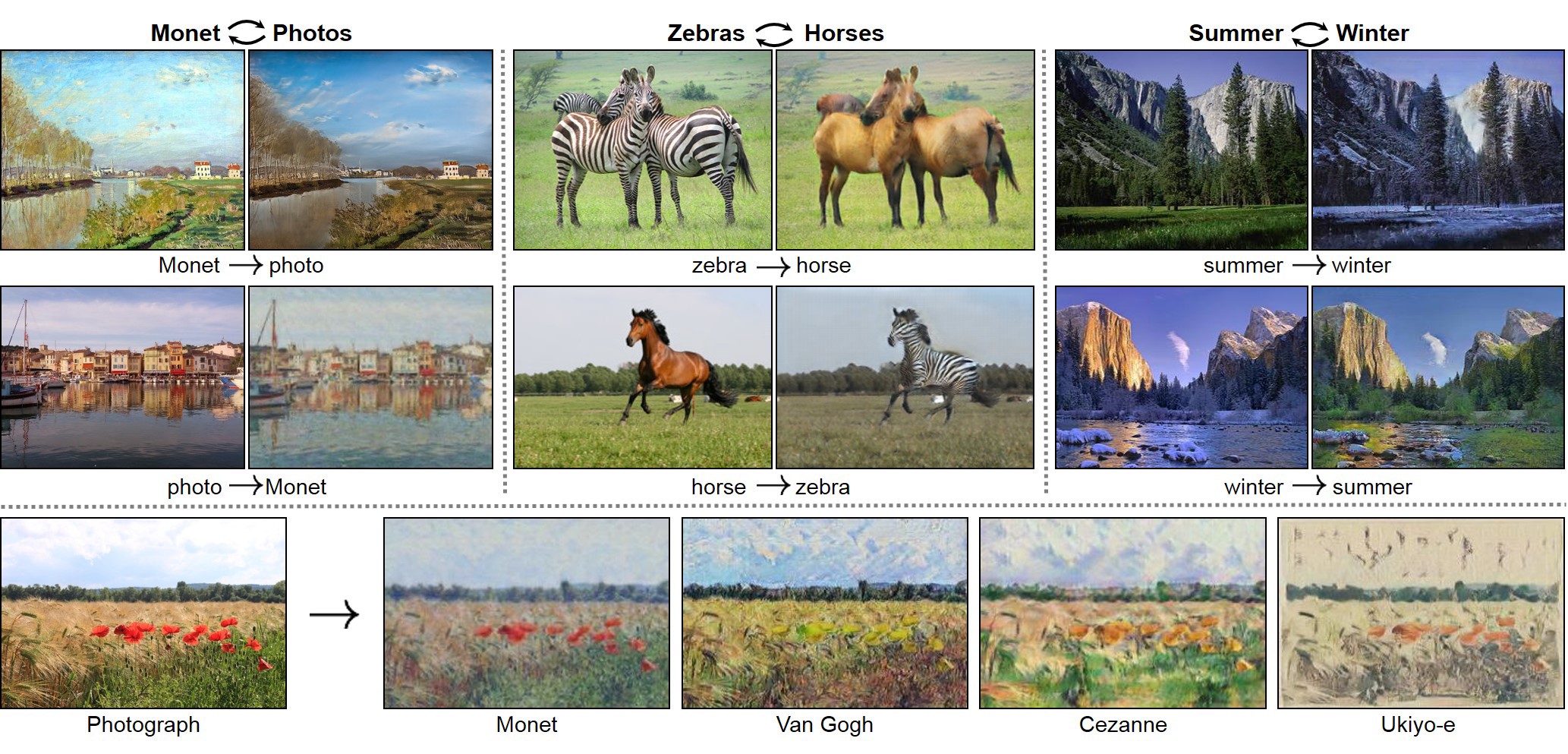{width=600px}
* Self play{width=600px}
* GAN:{width=600px}
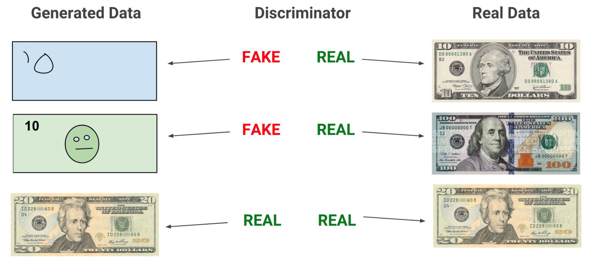{width=600px}
* Value function of GAN $$ \min_G \max_D V(D, G) = \mathbb{E}_{x \sim p_{\text{data}}(x)} [\log D(x)] + \mathbb{E}_{z \sim p_z(z)} [\log (1 - D(G(z)))]. $$ * Training GAN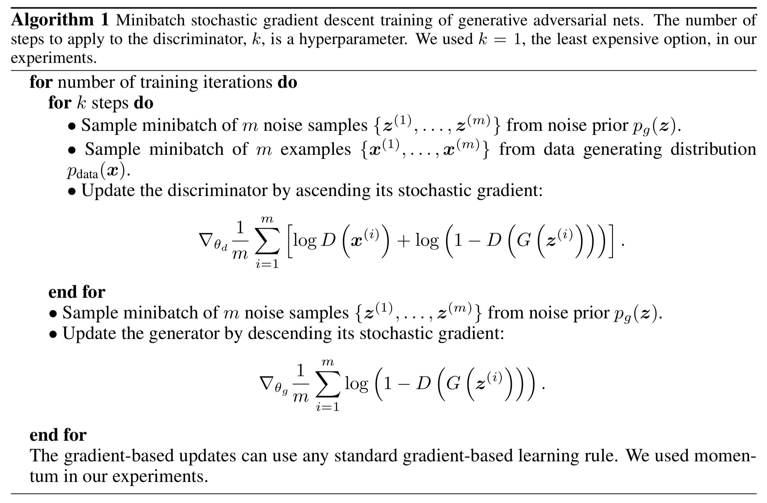{width=600px}