---
title: "Data Visualization With ggplot2 (and Seaborn)"
subtitle: Biostat 203B
author: "Dr. Hua Zhou @ UCLA"
date: "`r format(Sys.time(), '%d %B, %Y')`"
format:
  html:
    theme: cosmo
    number-sections: true
    toc: true
    toc-depth: 4
    toc-location: left
    code-fold: false
bibliography: "../bib-HZ.bib"
csl: "../apa.csl"
knitr:
  opts_chunk: 
    fig.align: 'center'
    fig.width: 6
    fig.height: 4
    message: FALSE
    cache: false
---

Display machine information for reproducibility.

::: {.panel-tabset}

#### R

```{r}
sessionInfo()
```

#### Python

```{python}
import IPython
print(IPython.sys_info())
```

:::

We use the ggplot2 package in tidyverse for static visualization. The closest thing in Python is the [plotnine](https://plotnine.readthedocs.io/en/stable/index.html#) library. But we mostly use [Seaborn](https://seaborn.pydata.org/) library, which is based on [matplotlib](https://matplotlib.org/), due to its popularity in the Python data science community. For Julia users, I recommend [Makie.jl](https://docs.makie.org/stable/).

::: {.panel-tabset}

#### R

```{r}
library(tidyverse)
```

#### Python

```{python}
# Load the pandas library
import pandas as pd
# Load numpy for array manipulation
import numpy as np
# Load seaborn plotting library
import seaborn as sns
import matplotlib.pyplot as plt

# Set font sizes in plots
sns.set(font_scale = 1.25)
# Display all columns
pd.set_option('display.max_columns', None)
```

:::

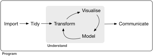
A typical data science project:

<p align="center">
<img src="./data-science.png" height="300">
</p>

## Data visualization

> “The simple graph has brought more information to the data analyst’s mind than any other device.”  
> 
> John Tukey

## `mpg` data

::: {.panel-tabset}

#### R

- `mpg` data is available from the `ggplot2` package:

```{r}
mpg %>% print(width = Inf)
```
- Tibbles are a generalized form of data frames, which are extensively used in tidyverse.

#### Python

- `mpg` data is available from the `plotline` package:

```{python}
from plotnine.data import mpg

mpg
mpg.info()
```

Note the `mpg` data in Seaborn is different from that in ggplot2: different number of samples and different variable namees. 
```{python}
sns.load_dataset("mpg").shape
sns.load_dataset("mpg").info()
```

:::
    
- `displ`: engine size, in liters.  
    `hwy`: highway fuel efficiency, in mile per gallon (mpg).

## Aesthetic mappings | r4ds chapter 3.3
    
### Scatter plot

- `hwy` vs `displ` 

::: {.panel-tabset}

#### R

```{r}
ggplot(data = mpg) + 
  geom_point(mapping = aes(x = displ, y = hwy))
```

#### Python

```{python}
plt.figure()
sns.relplot(
  data = mpg,
  kind = "scatter",
  x = "displ",
  y = "hwy"
);
plt.show()
```

:::

- An aesthetic maps data to a specific feature of plot. 

- Check available aesthetics for a geometric object by `?geom_point`.

### Color of points

- Color points according to `class`:

::: {.panel-tabset}

#### R

```{r}
ggplot(data = mpg) + 
  geom_point(mapping = aes(x = displ, y = hwy, color = class))
```

#### Python

```{python}
plt.figure()
sns.relplot(
  data = mpg,
  kind = "scatter",
  x = "displ",
  y = "hwy",
  hue = "class",
  height = 8
);
plt.show()
```

:::

### Size of points 

- Assign different sizes to points according to `class`:

::: {.panel-tabset}

#### R

```{r}
#| warning: false
ggplot(data = mpg) + 
  geom_point(mapping = aes(x = displ, y = hwy, size = class))
```

#### Python

Better to reverse the order, using `size_order` argument.
```{python}
plt.figure()
sns.relplot(
  data = mpg,
  kind = "scatter",
  x = "displ",
  y = "hwy",
  size = "class",
  size_order = np.sort(np.unique(mpg['class']))[::-1],
  height = 8
);
plt.show()
```

:::

### Transparency of points 

- Assign different transparency levels to points according to `class`:

::: {.panel-tabset}

#### R

```{r}
ggplot(data = mpg) + 
  geom_point(mapping = aes(x = displ, y = hwy, alpha = class))
```

#### Python (???)

The `alpha` argument in Seaborn only takes a number. I don't know how to do it elegantly, besides stacking different levels of points.

```{python}
plt.figure()
# alphas mapping to each level of class
cats = mpg['class'].unique() # levels sorted
alphas = np.linspace(0, 1, num = cats.size + 2)[1:-1]
_, ax = plt.subplots()
for cls, alpha in zip(cats, alphas):
  sns.scatterplot(
    data = mpg[mpg['class'] == cls],
    x = "displ",
    y = "hwy",
    alpha = alpha,
    ax = ax
    );
ax.legend(
  labels = cats,
  fontsize = 16
  )    
plt.show()
```

:::


### Shape of points (markers)

- Assign different shapes to points according to `class`:

::: {.panel-tabset}

#### R

```{r}
#| warning: false
ggplot(data = mpg) + 
  geom_point(mapping = aes(x = displ, y = hwy, shape = class))
```

- Maximum of 6 shapes at a time. By default, additional groups will go unplotted.

#### Python

```{python}
plt.figure()
sns.relplot(
  data = mpg,
  kind = "scatter",
  x = "displ",
  y = "hwy",
  style = "class",
  # marker size
  s = 20, 
  height = 8
);
plt.show()
```

:::

### Manual setting of an aesthetic 

- Set the color of all points to be blue:

::: {.panel-tabset}

#### R

```{r}
ggplot(data = mpg) + 
  geom_point(mapping = aes(x = displ, y = hwy), color = "blue")
```

#### Python

```{python}
plt.figure()
sns.relplot(
  data = mpg,
  kind = "scatter",
  x = "displ",
  y = "hwy",
  color = "blue", # matplotlib argument
  height = 8
);
plt.show()
```

:::

## Facets | r4ds chapter 3.5

### Facets 

- Facets divide a plot into subplots based on the values of one or more discrete variables.

::: {.panel-tabset}

#### R

- A subplot for each car type:
```{r}
ggplot(data = mpg) + 
  geom_point(mapping = aes(x = displ, y = hwy)) + 
  facet_wrap(~ class, nrow = 2)
```

- A subplot for each car type and drive:
```{r}
ggplot(data = mpg) + 
  geom_point(mapping = aes(x = displ, y = hwy)) + 
  facet_grid(drv ~ class)
```

#### Python

- A subplot for each car type:
```{python}
plt.figure()
sns.relplot(
  data = mpg,
  kind = "scatter",
  x = "displ",
  y = "hwy",
  # Variables that define subsets to plot on different facets
  col = "class",
  col_wrap = 4
);
plt.show()
```

- A subplot for each car type and drive:

```{python}
sns.relplot(
  data = mpg,
  kind = "scatter",
  x = "displ",
  y = "hwy",
  # Variables that define subsets to plot on different facets
  col = "class",
  row = "drv"
);
plt.show()
```

:::

## Geometric objects | r4ds chapter 3.6

### `geom_smooth()`: smooth line

- `hwy` vs `displ` line:

::: {.panel-tabset}

#### R

```{r}
ggplot(data = mpg) + 
  geom_smooth(mapping = aes(x = displ, y = hwy))
```

#### Python (???)

We can use [`lmplot`](https://seaborn.pydata.org/generated/seaborn.lmplot.html#seaborn.lmplot) (figure-level function) or [`regplot`](https://seaborn.pydata.org/generated/seaborn.regplot.html) (axes-level functions) for regression lines.

The lowess curve looks different from ggplot2. [How to pass lowess parameters to the statsmodels package under the hood?](https://github.com/mwaskom/seaborn/issues/2351)

Confidence intervals cannot currently be drawn for this kind of model.
```{python}
plt.figure()
sns.lmplot(
  data = mpg,
  x = "displ",
  y = "hwy",
  scatter = False,
  lowess = True
);
plt.show()
```

:::

### Different line types

- Different line types according to `drv`:

::: {.panel-tabset}

#### R

```{r}
ggplot(data = mpg) + 
  geom_smooth(mapping = aes(x = displ, y = hwy, linetype = drv))
```

#### Python (???)

I don't know how to map line styles to a categorical variable elegantly, besides doing a dumb loop.
```{python}
plt.figure()
drvs = np.sort(mpg['drv'].unique()) # levels sorted: '4', 'f', 'r'
ls = ["-", "--", "-."] # ["solid", "dashed", "dashdot"]
_, ax = plt.subplots()
for dr, ls in zip(drvs, ls):
  sns.regplot(
    data = mpg[mpg['drv'] == dr],
    x = "displ",
    y = "hwy",
    scatter = False,
    lowess = True,
    line_kws = {"ls": ls},
    ax = ax,
  )
ax.legend(
  labels = drvs,
  fontsize = 16
  )
plt.show()
```

:::

### Different line colors

- Different line colors according to `drv`:

::: {.panel-tabset}

#### R

```{r}
ggplot(data = mpg) + 
  geom_smooth(mapping = aes(x = displ, y = hwy, color = drv))
```

#### Python

```{python}
plt.figure()
sns.lmplot(
  data = mpg,
  x = "displ",
  y = "hwy",
  hue = "drv",
  scatter = False,
  lowess = True
);
plt.show()
```

:::

### Points and lines (together)

::: {.panel-tabset}

#### R

- Lines overlaid over scatter plot:
```{r}
ggplot(data = mpg) + 
  geom_point(mapping = aes(x = displ, y = hwy)) + 
  geom_smooth(mapping = aes(x = displ, y = hwy))
```

- Same as
```{r}
ggplot(data = mpg, mapping = aes(x = displ, y = hwy)) + 
  geom_point() + geom_smooth()
```

#### Python

The keyword argument `scatter` in the `lmplot` or `regplot` functions turns on or off scatter plot, besides the line plot 
```{python}
plt.figure()
sns.lmplot(
  data = mpg,
  x = "displ",
  y = "hwy",
  scatter = True,
  lowess = True
);
plt.show()
```

:::


### Aesthetics for each geometric object

- Different aesthetics in different layers:

::: {.panel-tabset}

#### R

```{r}
ggplot(data = mpg, mapping = aes(x = displ, y = hwy)) + 
  # Different color for each class
  geom_point(mapping = aes(color = class)) + 
  # Only display the line for subcompact cars
  geom_smooth(data = mpg %>% filter(class == "subcompact"), se = FALSE)
```

#### Python

```{python}
plt.figure()
ax = sns.scatterplot(
  data = mpg,
  x = "displ",
  y = "hwy"
);
sns.regplot(
  data = mpg[mpg['class'] == "subcompact"],
  x = "displ",
  y = "hwy",
  scatter = False,
  lowess = True,
  ax = ax
);
plt.show()
```

:::

## Jitter

Jitter adds random noise to X and Y position of each element to avoid over-plotting.

::: {.panel-tabset}

#### R

- `position = "jitter"` adds random noise to X and Y position of each element to avoid over-plotting:  
```{r}
ggplot(data = mpg) + 
  geom_point(mapping = aes(x = displ, y = hwy), position = "jitter")
```

- `geom_jitter()` is similar:  
```{r}
ggplot(data = mpg) + 
  geom_jitter(mapping = aes(x = displ, y = hwy))
```

#### Python (???)

I can only use the `stripplot` to achieve something similar. It treats the `displ` variable as a categorical variable.
```{python}
plt.figure()
sns.stripplot(
  data = mpg,
  x = "displ",
  y = "hwy",
  jitter = 0.5,
  size = 2.5,
  color = "black",
  native_scale = True
)
plt.show()
```

:::

## Bar plots | r4ds chapter 3.7

### `diamonds` data 

- `diamonds` data:

::: {.panel-tabset}

#### R

```{r}
diamonds
```

#### Python

```{python}
from plotnine.data import diamonds

diamonds
diamonds.info()
```

:::

### Bar plot

::: {.panel-tabset}

#### R

- `geom_bar()` creates bar chart:
```{r}
ggplot(data = diamonds) + 
  geom_bar(mapping = aes(x = cut))
```

- Bar charts, like histograms, frequency polygons, smoothers, and boxplots, plot some computed variables instead of raw data.

- Check available computed variables for a geometric object via help:
```{r}
#| eval: false
?geom_bar
```

- Use `stat_count()` directly:
```{r}
ggplot(data = diamonds) + 
  stat_count(mapping = aes(x = cut))
```

- `stat_count()` has a default geom `geom_bar()`.

#### Python

It is called `countplot` in Seaborn!
```{python}
plt.figure()
sns.countplot(
  data = diamonds,
  x = "cut",
  # Single color
  color = "skyblue"
)
plt.show()
```
Or the newer `histplot`
```{python}
plt.figure()
sns.histplot(
  data = diamonds,
  x = "cut"
)
plt.show()
```

Another high-level, figure-level function for displaying categorical variables is [`catplot`](https://seaborn.pydata.org/tutorial/categorical.html). 

```{python}
plt.figure()
sns.catplot(
  data = diamonds,
  x = "cut",
  kind = "count"
);
plt.show()
```

:::


- Display frequency instead of counts:

::: {.panel-tabset}

#### R

```{r}
ggplot(data = diamonds) + 
  geom_bar(mapping = aes(x = cut, y = after_stat(prop), group = 1))    
```
Note the aesthetics mapping `group=1` overwrites the default grouping (by `cut`) by considering all observations as a group. Without this we get
```{r}
ggplot(data = diamonds) + 
  geom_bar(mapping = aes(x = cut, y = after_stat(prop)))
```

#### Python

```{python}
plt.figure()
sns.histplot(
  data = diamonds,
  x = "cut",
  stat = "probability",
  # shrink = .8
);
plt.show()
```

:::

- Color bar:

::: {.panel-tabset}

#### R

```{r, results = 'hold'}
ggplot(data = diamonds) + 
  geom_bar(mapping = aes(x = cut, colour = cut))
```

#### Python (???)

Not sure how to do this in Python.

:::

- Fill color: 

::: {.panel-tabset}

#### R

```{r, results = 'hold'}
ggplot(data = diamonds) + 
  geom_bar(mapping = aes(x = cut, fill = cut))
```

#### Python

By default, `countplot` is already filling different colors for levels. For single color, use the `color` argument.

```{python}
plt.figure()
sns.countplot(
  data = diamonds,
  x = "cut"
)
plt.show()
```

:::


- Fill color according to another variable:

::: {.panel-tabset}

#### R

```{r}
ggplot(data = diamonds) + 
  geom_bar(mapping = aes(x = cut, fill = clarity))
```

#### Python (???)

Counts don't look right?
```{python}
plt.figure()
sns.histplot(
  data = diamonds,
  x = "cut",
  hue = "clarity",
  multiple = "stack"
)
plt.show()
```

:::

### `geom_bar()` vs `geom_col()`


::: {.panel-tabset}

#### R

- `geom_bar()` makes the height of the bar proportional to the number of cases in each group (or if the weight aesthetic is supplied, the sum of the weights).
```{r}
ggplot(data = diamonds) + 
  geom_bar(mapping = aes(x = cut))
```
The height of bar is the number of diamonds in each cut category.
    
- `geom_col()` makes the heights of the bars to represent values in the data.

```{r}
ggplot(data = diamonds) + 
  geom_col(mapping = aes(x = cut, y = carat))
```
The height of bar is total carat in each cut category.

#### Python

In `histplot` without `weights` argument, bar height is the count of each category.
```{python}
plt.figure()
sns.histplot(
  data = diamonds,
  x = "cut",
  weights = "carat"
)
plt.show()
```

`histplot` with `weights` argument set to the variable being counted/sumed.
```{python}
plt.figure()
sns.histplot(
  data = diamonds,
  x = "cut",
  weights = "carat"
)
plt.show()
```

:::

- `position_fill()` stack elements on top of one another,
normalize height:  

::: {.panel-tabset}

#### R

```{r}
ggplot(data = diamonds) + 
  geom_bar(mapping = aes(x = cut, fill = clarity), position = "fill")
```

#### Python (???)

Set `multiple` to `"fill"` in `histplot`:
```{python}
plt.figure()
sns.histplot(
  data = diamonds,
  x = "cut",
  hue = "clarity",
  multiple = "fill"
)
plt.show()
```

:::

- `position_dodge()` arrange elements side by side:  

::: {.panel-tabset}

#### R

```{r}
ggplot(data = diamonds) + 
  geom_bar(mapping = aes(x = cut, fill = clarity), position = "dodge")
```

#### Python

Set `multiple` argument to `dodge` in `histplot`.
```{python}
plt.figure()
sns.histplot(
  data = diamonds,
  x = "cut",
  hue = "clarity",
  multiple = "dodge"
)
plt.show()
```

:::

- `position_stack()` stack elements on top of each other:  

::: {.panel-tabset}

#### R

```{r}
ggplot(data = diamonds) + 
  geom_bar(mapping = aes(x = cut, fill = clarity), position = "stack")
```

#### Python

Why the counts look different?
```{python}
plt.figure()
sns.histplot(
  data = diamonds,
  x = "cut",
  hue = "clarity",
  multiple = "layer"
)
plt.show()
```

:::

## Box plots, violin plots

- Recall the mpg data:

::: {.panel-tabset}

#### R

```{r}
mpg
```

#### Python

```{python}
mpg
```

:::


- Boxplots (grouped by class):

::: {.panel-tabset}

#### R

Default:
```{r}
ggplot(data = mpg, mapping = aes(x = class, y = hwy)) + 
  geom_boxplot()
```
Add notches:
```{r}
ggplot(data = mpg, mapping = aes(x = class, y = hwy)) + 
  geom_boxplot(notch = TRUE)
```


#### Python

Default:
```{python}
plt.figure()
sns.boxplot(
  data = mpg,
  x = 'class',
  y = 'hwy',
)
plt.show()
```

Add notches:
```{python}
plt.figure()
sns.boxplot(
  data = mpg,
  x = 'class',
  y = 'hwy',
  notch = True
)
plt.show()
```

:::

- Violin plots (grouped by class):

::: {.panel-tabset}

#### R

```{r}
ggplot(data = mpg, mapping = aes(x = class, y = hwy)) + 
  geom_violin()
```

#### Python

```{python}
plt.figure()
sns.violinplot(
  data = mpg,
  x = 'class',
  y = 'hwy',
)
plt.show()
```

:::

## Coordinate systems | r4ds chapter 3.9

- `coord_cartesian()` is the default Cartesian coordinate system:

::: {.panel-tabset}

#### R

```{r}
ggplot(data = mpg, mapping = aes(x = class, y = hwy)) + 
  geom_boxplot() + 
  coord_cartesian(xlim = c(0, 5))
```

#### Python

Set xlim:
```{python}
plt.figure()
sns.boxplot(
  data = mpg,  
  x = "class",
  y = "hwy"
).set_xlim(-2, 7);
plt.show()
```

:::

- `coord_fixed()` specifies aspect ratio (x / y):

::: {.panel-tabset}

#### R

```{r}
ggplot(data = mpg, mapping = aes(x = class, y = hwy)) + 
  geom_boxplot() + 
  coord_fixed(ratio = 1/2)
```

#### Python

`catplot` function accepts the `aspect` argument for aspect ratio.
```{python}
plt.figure()
sns.catplot(
  data = mpg,  
  x = "class",
  y = "hwy",
  kind = "box",
  aspect = 0.5
)
plt.show()
```

::: 

- `coord_flip()` flips x- and y- axis:

::: {.panel-tabset}

#### R

```{r}
ggplot(data = mpg, mapping = aes(x = class, y = hwy)) + 
  geom_boxplot() + 
  coord_flip()
```

#### Python

Just need to flip the x and y arguments! Looks much nicer.
```{python}
plt.figure()
sns.catplot(
  data = mpg,  
  y = "class",
  x = "hwy",
  kind = "box"
)
plt.show()
```

:::

- Pie chart:

::: {.panel-tabset}

#### R

```{r}
ggplot(data = mpg, mapping = aes(x = factor(1), fill = class)) + 
  geom_bar(width = 1) + 
  coord_polar("y")
```

#### Python

Seaborn does not have a function for pie chart. Let's use Pandas groupby and matplotlib.

```{python}
plt.figure()
mpg.groupby("class").size().plot.pie(autopct = "%.1f%%")
plt.show()
```

:::

- A map:
```{r}
library("maps")
nz <- map_data("nz")
head(nz, 20)
```

```{r}
ggplot(nz, aes(x = long, y = lat, group = group)) +
  geom_polygon(fill = "white", colour = "black")
```


- `coord_quickmap()` puts maps in scale:
```{r}
ggplot(nz, aes(long, lat, group = group)) +
  geom_polygon(fill = "white", colour = "black") +
  coord_quickmap()
```

## Maps

More extensive mapping functions are provided in `ggmap` package in R.

```{r}
library(ggmap)

# Path from LA to Yosemite
trek_df <- trek(
  from = "los angeles, california", 
  to = "yosemite, california", 
  structure = "route"
  )
qmap("california", zoom = 7) +
  geom_path(
    aes(x = lon, y = lat),
    colour = "blue",
    linewidth = 1.5, 
    alpha = .5,
    data = trek_df, 
    lineend = "round"
  )
```

Python users check the [`Cartopy`](https://scitools.org.uk/cartopy/docs/latest/) package.

```{python}
import cartopy.crs as ccrs

plt.figure()
ax = plt.axes(projection=ccrs.Mollweide())
ax.stock_img()
plt.show()
```

For interactive maps, use `leaflet`!
```{r}
library(leaflet)

leaflet() %>%
  addTiles() %>%  # Add default OpenStreetMap map tiles
  addMarkers(lng = -118.44481, lat = 34.07104, popup = "Bruin")
```

## Graphics for communications | r4ds chapter 28

### Title 

- Figure title should be descriptive:

::: {.panel-tabset}

#### R

```{r}
ggplot(mpg, aes(x = displ, y = hwy)) +
  geom_point(aes(color = class)) +
  geom_smooth(se = FALSE) +
  labs(title = "Fuel efficiency generally decreases with engine size")
```

#### Python

```{python}
plt.figure()
sns.relplot(
  data = mpg,
  kind = "scatter",
  x = "displ",
  y = "hwy"
).set(
  title = "Fuel efficiency generally decreases with engine size"
)
plt.show()
```
:::

### Subtitle and caption 

::: {.panel-tabset}

#### R

```{r}
ggplot(mpg, aes(displ, hwy)) +
  geom_point(aes(color = class)) +
  geom_smooth(se = FALSE) + 
  labs(
    title = "Fuel efficiency generally decreases with engine size",
    subtitle = "Two seaters (sports cars) are an exception because of their light weight",
    caption = "Data from fueleconomy.gov"
  )
```

#### Python

```{python}
plt.figure()
sns.relplot(
  data = mpg,
  kind = "scatter",
  x = "displ",
  y = "hwy"
).set(
  title = "Fuel efficiency generally decreases with engine size"
)
plt.suptitle("Two seaters (sports cars) are an exception because of their light weight", fontsize = 12)
plt.show()
```

:::

### Axis labels 

::: {.panel-tabset}

#### R

```{r}
ggplot(mpg, aes(displ, hwy)) +
  geom_point(aes(colour = class)) +
  geom_smooth(se = FALSE) +
  labs(
    x = "Engine displacement (L)",
    y = "Highway fuel economy (mpg)"
  )
```

#### Python

```{python}
plt.figure()
sns.regplot(
  data = mpg,
  x = "displ",
  y = "hwy",
  scatter = True,
  lowess = True
).set(
  xlabel = "Engine displacement (L)",
  ylabel = "Highway fuel economy (mpg)"
)
plt.show()
```

:::

### Math equations 

::: {.panel-tabset}

#### R

```{r}
df <- tibble(x = runif(10), y = runif(10))
ggplot(df, aes(x, y)) + geom_point() +
  labs(
    x = quote(sum(x[i] ^ 2, i == 1, n)),
    y = quote(alpha + beta + frac(delta, theta))
  )
```

- `?plotmath` 

#### Python

```{python}
plt.figure()
df = pd.DataFrame({
  'x': np.random.rand(10),
  'y': np.random.rand(10)
})
sns.regplot(
  data = df,
  x = "x",
  y = "y"
).set(
  xlabel = r'$\sum_1^n x_i^2$',
  ylabel = r'$\alpha + \beta + \frac{\delta}{\theta}$'
)
plt.show()
```

:::

### Annotations 

::: {.panel-tabset}

#### R

- Find the most fuel efficient car in each car class:

```{r}
best_in_class <- mpg %>%
  group_by(class) %>%
  filter(row_number(desc(hwy)) == 1)
best_in_class
```

- Annotate points
```{r}
ggplot(mpg, aes(x = displ, y = hwy)) +
  geom_point(aes(colour = class)) +
  geom_text(aes(label = model), data = best_in_class)
```

- `ggrepel` package automatically adjusts labels so that they don’t overlap:
```{r}
library("ggrepel")

ggplot(mpg, aes(displ, hwy)) +
  geom_point(aes(colour = class)) +
  geom_point(size = 3, shape = 1, data = best_in_class) +
  ggrepel::geom_label_repel(aes(label = model), data = best_in_class)
```
 
#### Python (???)

I don't know easy way to annotate, besides writing a loop.
```{python}
# Locate the most efficient car in each class
best_in_class = mpg.sort_values(
  by = 'hwy', 
  ascending = False
  ).groupby('class').first()
best_in_class
```

```{python}
plt.figure()
# Regression line
sns.relplot(
  data = mpg,
  x = "displ",
  y = "hwy",
  hue = "class"
)
# Loop to add text annotation
for i in range(0, best_in_class.shape[0]):
  plt.text(
    x = best_in_class.displ[i],
    y = best_in_class.hwy[i],
    s = best_in_class.model[i]
    )
plt.show()
```

:::

### Scales

```{r}
#| eval: false
ggplot(mpg, aes(displ, hwy)) +
  geom_point(aes(colour = class))
```
automatically adds scales
```{r}
ggplot(mpg, aes(displ, hwy)) +
  geom_point(aes(colour = class)) +
  scale_x_continuous() +
  scale_y_continuous() +
  scale_colour_discrete()
```

- `breaks`

::: {.panel-tabset}

#### R

```{r}
ggplot(mpg, aes(displ, hwy)) +
  geom_point() +
  scale_y_continuous(breaks = seq(15, 40, by = 5))
```

#### Python

```{python}
plt.figure()
sns.scatterplot(
  data = mpg,
  x = "displ",
  y = "hwy"
).set_yticks(
  np.arange(start = 15, stop = 41, step = 5)
)
plt.show()
```

:::


- `labels`

::: {.panel-tabset}

#### R

```{r}
ggplot(mpg, aes(displ, hwy)) +
  geom_point() +
  scale_x_continuous(labels = NULL) +
  scale_y_continuous(labels = NULL)
```

#### Python

```{python}
plt.figure()
ax = sns.scatterplot(
  data = mpg,
  x = "displ",
  y = "hwy"
)
ax.set_xticklabels([])
ax.set_yticklabels([])
plt.show()
```

:::

- Plot y-axis at log scale:

::: {.panel-tabset}

#### R

```{r}
ggplot(mpg, aes(x = displ, y = hwy)) +
  geom_point() +
  scale_y_log10()
```

#### Python

```{python}
plt.figure()
ax = sns.scatterplot(
  data = mpg,
  x = "displ",
  y = "hwy"
).set_yscale("log")
plt.show()
```

:::

- Plot x-axis in reverse order:

::: {.panel-tabset}

#### R

```{r}
ggplot(mpg, aes(x = displ, y = hwy)) +
  geom_point() +
  scale_x_reverse()
```

#### Python

```{python}
plt.figure()
ax = sns.scatterplot(
  data = mpg,
  x = "displ",
  y = "hwy"
).invert_xaxis()
plt.show()
```

:::
    
### Legends

::: {.panel-tabset}

#### R

- Set legend position: `"left"`, `"right"`, `"top"`, `"bottom"`, `none`:
```{r}
#| collapse: true
ggplot(mpg, aes(displ, hwy)) +
  geom_point(aes(colour = class)) + 
  theme(legend.position = "left")
```

- See following link for more details on how to change title, labels, ... of a legend.

    <http://www.sthda.com/english/wiki/ggplot2-legend-easy-steps-to-change-the-position-and-the-appearance-of-a-graph-legend-in-r-software> 

#### Python

```{python}
plt.figure()
ax = sns.scatterplot(
  data = mpg,
  x = "displ",
  y = "hwy",
  hue = "class"
)
plt.legend(loc = "upper left")
plt.show()
```

:::


### Zooming

- Without clipping (calculate smoothing line using all data points)

::: {.panel-tabset}

#### R

```{r}
ggplot(mpg, mapping = aes(displ, hwy)) +
  geom_point(aes(color = class)) +
  geom_smooth() +
  coord_cartesian(xlim = c(5, 7), ylim = c(10, 30))
```

#### Python

```{python}
plt.figure()
ax = sns.regplot(
  data = mpg,
  x = "displ",
  y = "hwy",
  scatter = True,
  lowess = True,
)
ax.set_xlim(left = 5, right = 7)
ax.set_ylim(bottom = 10, top = 30)
plt.show()
```

:::

- With clipping (calculate smoothing line ignoring unseen data points)

::: {.panel-tabset}

#### R

```{r, message = FALSE, warning = FALSE}
ggplot(mpg, mapping = aes(displ, hwy)) +
  geom_point(aes(color = class)) +
  geom_smooth() +
  xlim(5, 7) + ylim(10, 30)
```

```{r, message = FALSE, warning = FALSE}
ggplot(mpg, mapping = aes(displ, hwy)) +
  geom_point(aes(color = class)) +
  geom_smooth() +
  scale_x_continuous(limits = c(5, 7)) +
  scale_y_continuous(limits = c(10, 30))
```

```{r, message = FALSE}
mpg %>%
  filter(displ >= 5, displ <= 7, hwy >= 10, hwy <= 30) %>%
  ggplot(aes(displ, hwy)) +
  geom_point(aes(color = class)) +
  geom_smooth()
```

#### Python

```{python}
plt.figure()
sns.regplot(
  data = mpg[(mpg["displ"] >= 5) & (mpg["displ"] <= 7) & (mpg["hwy"] >= 10) & (mpg["hwy"] <= 30)],
  x = "displ",
  y = "hwy",
  scatter = True,
  lowess = True,
)
plt.show()
```

:::

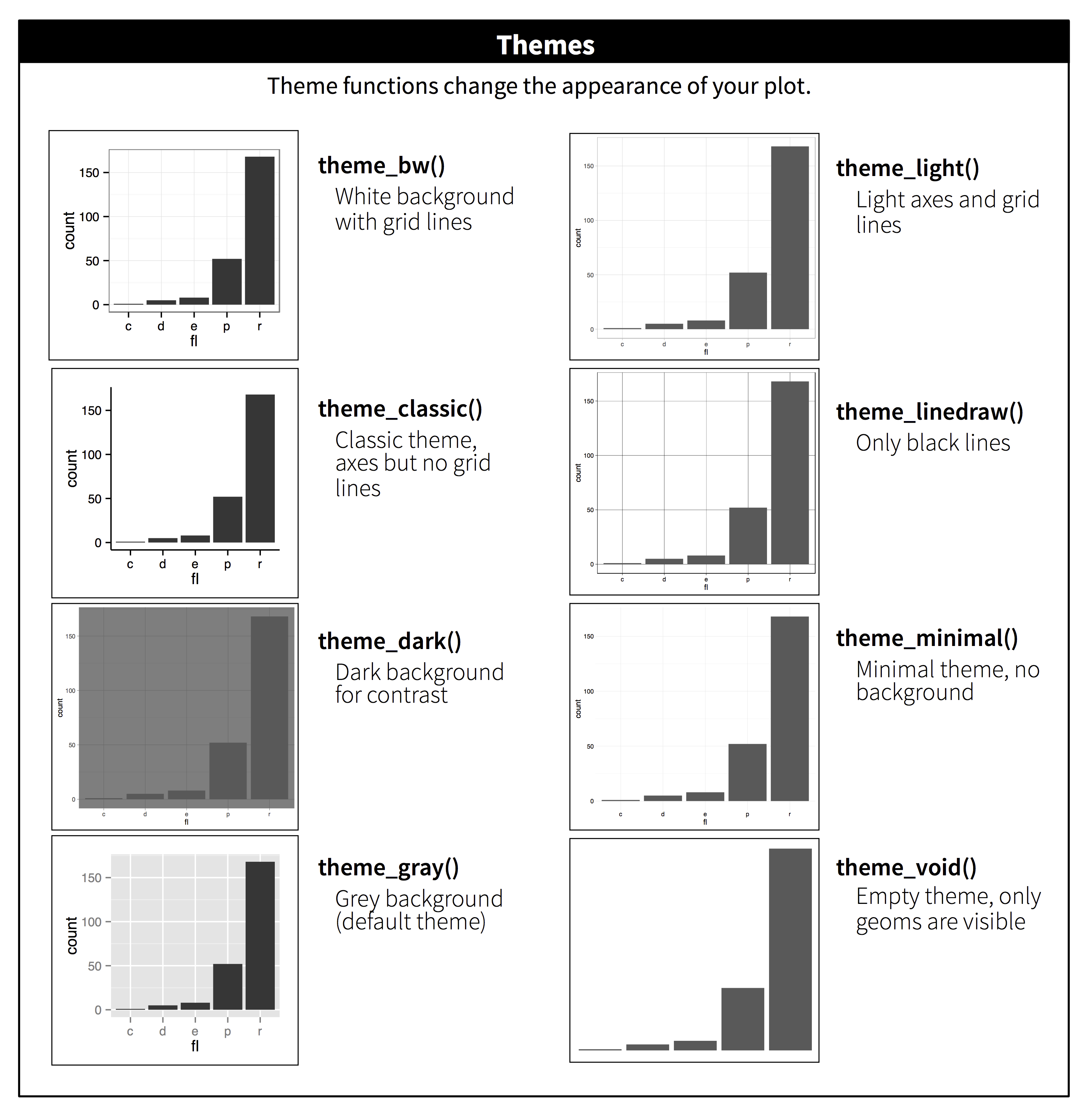
### Themes

::: {.panel-tabset}

#### R

<p align="center">
<img src="./visualization-themes.png" height="550">
</p>

```{r, message = FALSE}
ggplot(mpg, aes(displ, hwy)) +
  geom_point(aes(color = class)) +
  geom_smooth(se = FALSE) +
  theme_bw()
```

Many options exist in the `theme()` function for specific customization 
```{r, message = FALSE}
ggplot(mpg, aes(displ, hwy)) +
  geom_point(aes(color = class)) +
  geom_smooth(se = FALSE) +
  theme(
    legend.position = c(0.85, 0.85), 
    legend.key = element_blank(), 
    axis.text.x = element_text(angle = 0, size = 12), 
    axis.text.y = element_text(angle=0, size = 12), 
    axis.ticks = element_blank(), 
    legend.text=element_text(size = 8),
    panel.grid.major = element_blank(), 
    panel.border = element_blank(), 
    panel.grid.minor = element_blank(), 
    panel.background = element_blank(), 
    axis.line = element_line(color = 'black', linewidth = 0.3), 
    text = element_text(size = 13)
    )
```

#### Python

There are five preset seaborn themes: `darkgrid`, `whitegrid`, `dark`, `white`, and `ticks`. They are each suited to different applications and personal preferences. The default theme is `darkgrid`.

```{python}
sns.set_style("white")

plt.figure()
ax = sns.regplot(
  data = mpg,
  x = "displ",
  y = "hwy",
  scatter = True,
  lowess = True,
)
plt.show()
```

:::

::: {.callout-tip}
For academic papers, use the `white` theme in Seaborn or `theme_bw` in ggplot2.
:::

### Manual Colors

You may want to manually enter colors instead of relying on default colors. There is a [tool to pick optimally distinct colors](https://medialab.github.io/iwanthue/) that is useful. 

::: {.panel-tabset}

#### R

Manually select colors to use 

```{r, message = FALSE}
ggplot(filter(mpg, class == "suv" | class== "compact" |
                class == "pickup" | class == "minivan"), 
       aes(displ, hwy)) +
  geom_point(aes(color = class)) +
  theme_bw() + 
  scale_color_manual(values = c("#24aad8",
  "#cb6450",
  "#80a14b",
  "#aa65ba")) 
```

Manually assign labels to each color

```{r, message = FALSE}
ggplot(filter(mpg, class == "suv" | class== "compact" |
                class == "pickup" | class == "minivan"), 
       aes(displ, hwy)) +
  geom_point(aes(color = class)) +
  theme_bw() + 
  scale_color_manual(values = c(suv = "#24aad8",
                                pickup = "#cb6450",
                                minivan = "#80a14b",
                                compact = "#aa65ba")) 
```

#### Python

[Choose color palettes in Seaborn](https://seaborn.pydata.org/tutorial/color_palettes.html).

:::

### Saving plots

::: {.panel-tabset}

#### R

```{r, collapse = TRUE}
#| eval: false
ggplot(mpg, aes(displ, hwy)) + geom_point()
ggsave("my-plot.pdf")
```

#### Python

```{python}
#| eval: false
sns.scatterplot(
  data = mpg,
  x = "displ",
  y = "hwy"
).get_figure().savefig("my-plot.pdf")
```

:::

## Cheat sheet  

[RStudio cheat sheet](https://raw.githubusercontent.com/rstudio/cheatsheets/main/data-visualization.pdf) is extremely helpful.