---
title: "Import and Tidy Data"
subtitle: Biostat 203B
author: "Dr. Hua Zhou @ UCLA"
date: today
format:
  html:
    theme: cosmo
    embed-resources: true
    number-sections: true
    toc: true
    toc-depth: 4
    toc-location: left
    code-fold: false
knitr:
  opts_chunk: 
    fig.align: 'center'
---

## Outline

Display machine information for reproducibility.

::: {.panel-tabset}

#### R

```{r}
sessionInfo()
```

#### Python

```{python}
import IPython
print(IPython.sys_info())
```

#### Julia

```{julia}
#| eval: true
using InteractiveUtils
versioninfo()
```

:::


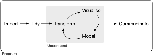
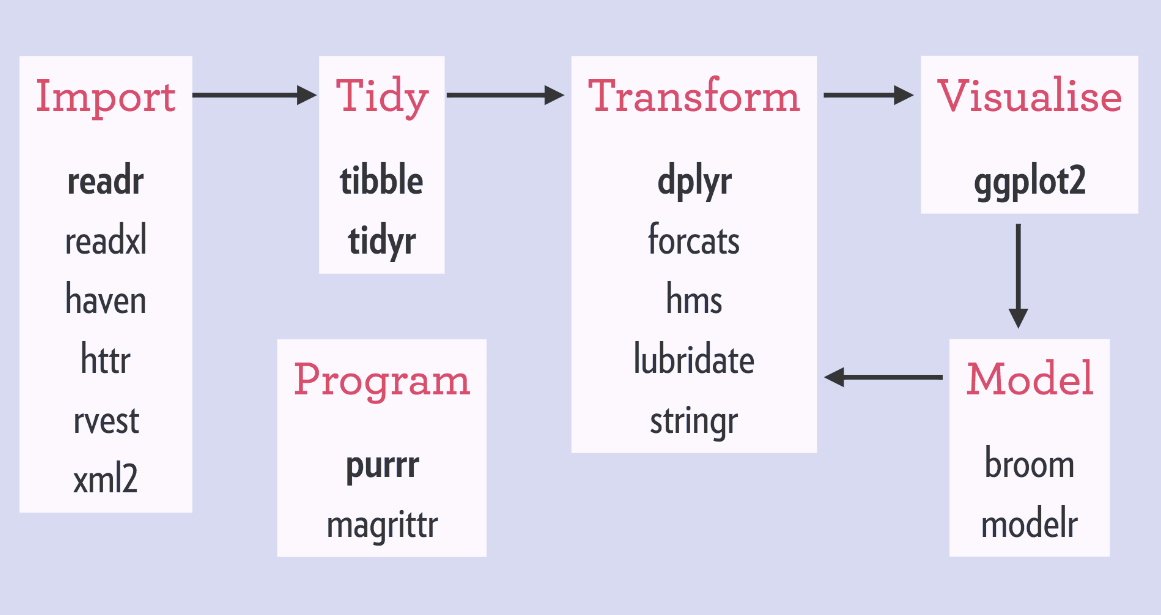
We will spend the next few weeks studying some R packages for typical data science projects.

* Data wrangling (import, tidy, visualization, transformation).
  * [R for Data Science (2ed)](https://r4ds.hadley.nz/) by Hadley Wickham, Mine Çetinkaya-Rundel, and Garrett Grolemund.
  * [_R Graphics Cookbook_](https://r-graphics.org) by Winston Chang. 

* Interactive data visualization by Shiny.

* Interface with databases, e.g., SQL, DuckDB, Google BigQuery, and Apache Spark.

* String and text data manipulation. 

* Web scraping.

A typical data science project:

<p align="center">
<img src="./data-science.png" height="300">
</p>

## Tidyverse

::: {.panel-tabset}

#### R

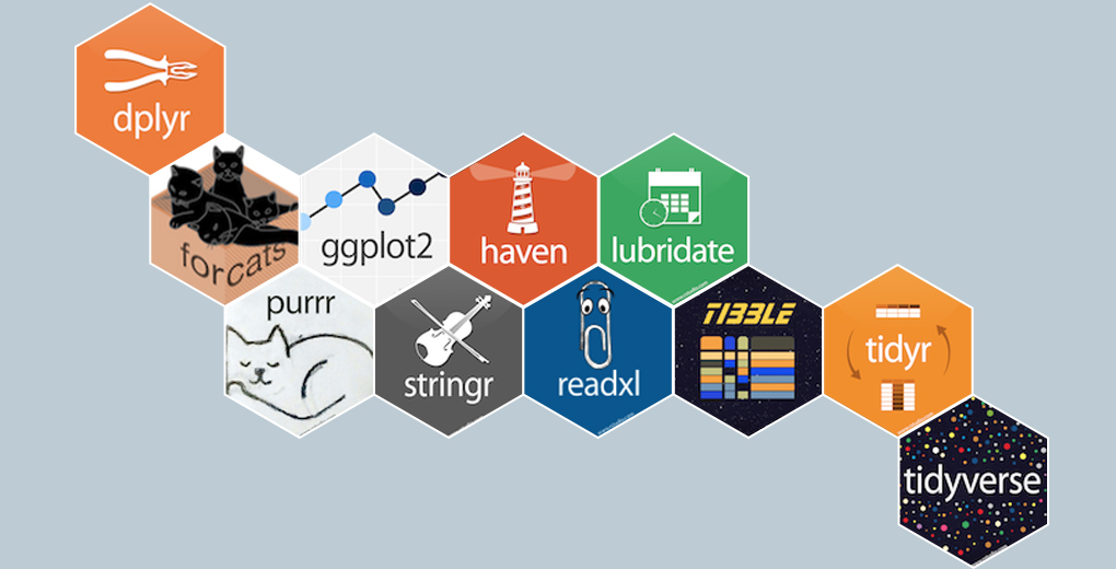
- [tidyverse](https://www.tidyverse.org/) is a collection of R packages for data ingestion, wrangling, and visualization.

<p align="center">
<img src="./tidyverse_pkgs.jpeg" width="450">
</p>

<p align="center">
<img src="./tidyverse_categories.png" width="450">
</p>

- The lead developer Hadley Wickham won the 2019 _COPSS Presidents’ Award_ (the Nobel Prize of Statistics) 

> for influential work in statistical computing, visualization, graphics, and data analysis; for developing and implementing an impressively comprehensive computational infrastructure for data analysis through R software; for making statistical thinking and computing accessible to large audience; and for enhancing an appreciation for the important role of statistics among data scientists.

- Install `tidyverse` from RStudio menu `Tools -> Install Packages...` or

```{r}
#| eval: false
install.packages("tidyverse")
```

- After installation, load `tidyverse` by

```{r}
library("tidyverse")
```

#### Python

The [pandas](https://pandas.pydata.org/) package is the Python analog of tidyverse.

![](https://pandas.pydata.org/static/img/pandas.svg){width=200}

Follow the [installation instructions](https://pandas.pydata.org/getting_started.html) to install pandas package in Python.

#### Julia

The [DataFrames.jl](https://github.com/JuliaData/DataFrames.jl) package and the [JuliaData ecosystem](https://github.com/JuliaData) is the Julia analog of tidyverse.

![](https://dataframes.juliadata.org/stable/assets/logo.png){width=200}

Install DataFrames.jl by:
```{julia}
#| eval: false
add DataFrames
```
in the package mode or
```{julia}
#| eval: false
using Pkg
Pkg.add("DatamFrames")
```
in Julia REPL.

:::

## Tibble | r4ds2e chapter 5

### Tibbles

- Tibbles extend data frames in R and form the core of tidyverse.

### Create tibbles

#### Convert between dataframe in base R and tibble

<p align="center">
<img src="./iris_dataset.jpg">
</p>

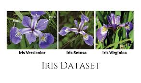
- `iris` is a data frame available in base R:

```{r}
# By default, R displays ALL rows of a regular data frame!
iris
```

```{r}
# Display structure of this data frame
str(iris)
```

- Convert a regular data frame to tibble, which by default only displays the first 10 rows of data.
```{r}
as_tibble(iris)
```
    
- Convert a tibble to data frame:
```{r}
#| eval: false
as.data.frame(tb)
```

#### Construct tibbles by columns

- Create tibble/dataframe from individual vectors.

::: {.panel-tabset}

#### R

Note values for `y` are recycled:
```{r}
tibble(
  x = 1:5, 
  y = 1, 
  z = x ^ 2 + y
)
```

#### Python

```{r}
reticulate::py_config()
```

```{python}
# Load the pandas library
import pandas as pd
# Load numpy for array manipulation
import numpy as np

# Create DataFrame from a dictionary
df = pd.DataFrame({
  'x': np.linspace(1, 5, 5), 
  'y': np.ones(5)
  })
df['z'] = df['x']**2 + df['y']
df
```

#### Julia

```{julia}
using DataFrames

df = DataFrame(
  x = 1:5,
  y = 1,
);
df[!, :z] = df[!, :x].^2 + df[!, :y];
df
```

:::

#### Construct tibbles by rows

- Transposed tibbles, or construct dataframe by rows:

::: {.panel-tabset}

#### R

```{r}
tribble(
  ~x, ~y, ~z,
  #--|--|----
  "a", 2, 3.6,
  "b", 1, 8.5
)
```

#### Python

```{python}
# Initialize list of lists
data = [['a', 2, 3.6], ['b', 1, 8.5]]
# Create DataFrame
df = pd.DataFrame(data, columns = ['x', 'y', 'z'])
df
```

#### Julia

In Julia, we can [build a DataFrame row by row](https://dataframes.juliadata.org/stable/man/getting_started/#Constructing-Row-by-Row) by `push`ing tuples
```{julia}
df = DataFrame(x = String[], y = Int[], z = Float64[]);
push!(df, ("a", 2, 3.6));
push!(df, ("b", 1, 8.5));
df
```
or dictionary
```{julia}
df = DataFrame(x = String[], y = Int[], z = Float64[]);
push!(df, Dict(:x => "a", :y => 2, :z => 3.6));
push!(df, Dict(:x => "b", :y => 1, :z => 8.5));
df
```
If you want to add rows at the beginning of a data frame use `pushfirst!` and to insert a row in an arbitrary location use `insert!`.

You can also add whole tables to a data frame using the `append!` and `prepend!` functions.

:::
  
### Printing of a tibble

::: {.panel-tabset}

#### R

- By default, tibble prints the first 10 rows and all columns _that fit on screen_.
```{r}
nycflights13::flights
```

- To change number of rows and columns to display:
```{r}
nycflights13::flights |> 
  print(n = 10, width = Inf)
```
Here we see the **pipe operator** `|>` pipes the output from previous command to the (first) argument of the next command.

::: {.callout-tip}
## Pipe operator

R 4.1.0 introduced a native pipe operator `|>`, which is mostly compatible with the pipe `%>%` offered by the tidyverse package magrittr. For some subtle differences, see this [post](https://www.tidyverse.org/blog/2023/04/base-vs-magrittr-pipe/) by Hadley Wickham.
:::

- To change the default print setting globally:
    - `options(tibble.print_max = n, tibble.print_min = m)`: if more than `m` rows, print only `n` rows.
    - `options(dplyr.print_min = Inf)`: print all row.
    - `options(tibble.width = Inf)`: print all columns.

#### Python

Pandas by default displays 10 rows and limits the number of columns to the display area.
```{python}
from nycflights13 import flights
flights
```
We can override this behavior by
```{python}
pd.set_option("display.max_rows", 50)
pd.set_option("display.max_columns", 20)

flights
```


#### Julia

By default DataFrames.jl limits the number of rows and columns when displaying a data frame in a Jupyter Notebook to 25 and 100, respectively. You can override this behavior by changing the values of the `ENV["DATAFRAMES_COLUMNS"]` and `ENV["DATAFRAMES_ROWS"]` variables to hold the maximum number of columns and rows of the output. All columns or rows will be printed if those numbers are equal or lower than 0.

:::

### Subsetting

#### Extract columns

::: {.panel-tabset}

#### R

- Create a tibble with two columns.
```{r}
df <- tibble(
  x = runif(5),
  y = rnorm(5)
)
df
```

- Extract a column by name:
```{r}
# Return a vector
df$x
# Return a vector
df[["x"]]
# Return a tibble
df[, "x"]
```

- Extract a column by position. Remember R indexing starts from 1!
```{r}
# Return a tibble
df[, 1] 
# Return a vector
df[[1]] 
```

- Pipe (it seems the base pipe `|>` does not support the following operations):
```{r}
# Return a vector
df %>% .$x
# Return a vector
df %>% .[["x"]]
```

- Access multiple columns at once.
```{r}
# Return a tibble
df[, c("x", "y")]
# Return a tibble
df[c("x", "y")]
# Return a tibble
df[c(1, 2)]
# Return a tibble
df %>% .[c("x", "y")]
```

#### Python

- Create a tibble with two columns.
```{python}
df = pd.DataFrame({
  'x': np.random.rand(5), 
  'y': np.random.randn(5)
  });
df
```

- Extract a column by name (`loc`):
```{python}
# Return a vector
df.loc[:, "x"]
```

- Extract a column by position (`iloc`). Remember Python indexing starts from 0!.
```{python}
# Return a vector
df.iloc[:, 0]
```

- Access multiple columns at once.
```{python}
# Return a DataFrame
df.loc[:, ['x', 'y']]
# Return a DataFrame
df.iloc[:, [0, 1]]
```

#### Julia

- Create a DataFrame with two columns.
```{julia}
df = DataFrame(x = rand(5), y = randn(5))
```

- Extract a column by name:
```{julia}
# Return a vector
df.x
# Return a vector
df."x"
# Return a vector
df[!, :x]  # does not make a copy
df[!, "x"] # does not make a copy
# Return a vector
df[:, :x]  # make a copy!
df[:, "x"] # make a copy!
```

- Extract a column by position. Remember Julia indexing starts from 1!
```{julia}
# Return a vector
df[!, 1]  # does not make a copy
# Return a vector
df[:, 1]  # make a copy!
```

- Pipe:
```{julia}
using Pipe

# Return a vector
@pipe df |> _[!, :x]
# Return a dataframe
@pipe df |> select(_, :x)
```

- Access multiple columns at once.
```{julia}
# Return a dataframe
df[!, [:x, :y]]
# Return a dataframe
@pipe df |> select(_, [:x, :y])
```
:::

#### Extract rows

::: {.panel-tabset}

#### R

Access row(s) by index(es).
```{r}
# Return a dataframe
df[1,]
```

Multiple rows.
```{r}
# Return a dataframe
df[1:3,]
```

#### Python

Access row(s) by index(es).
```{python}
# Return a vector
df.iloc[0]
```

Multiple rows.
```{python}
# Return a dataframe
df.iloc[[0, 1, 2]]
```

#### Julia

Access row(s) by index(es).
```{julia}
# Return a DataFrameRow
df[1, :]
```

Multiple rows.
```{julia}
# Return a dataframe
df[1:3, :]
```

:::

## Data import | r4ds2e chapter 7

### readr (R), pandas (Python), and CSV.jl (Julia)

- [readr](https://github.com/tidyverse/readr) package implements functions that ingest flat text files into tibbles.

    - `read_csv()`, `read_csv2()` (semicolon seperated files), `read_tsv()`,  `read_delim()`.

    - `read_fwf()` (fixed width files), `read_table()`.

    - `read_log()` (Apache style log files). 

- An example file [heights.csv](https://raw.githubusercontent.com/ucla-biostat-203b/2024winter/master/slides/05-tidy/heights.csv):
```{bash}
head heights.csv
```

::: {.panel-tabset}

#### R

- Read from a local file [heights.csv](https://raw.githubusercontent.com/ucla-biostat-203b/2024winter/master/slides/05-tidy/heights.csv):
```{r}
heights <- read_csv("heights.csv") |> print(width = Inf)
```

- `read_csv` can read gz file directly (HW2).

- Read from a url:
```{r}
heights <- read_csv("https://raw.githubusercontent.com/ucla-biostat-203b/2024winter/master/slides/05-tidy/heights.csv") |>
  print(width = Inf)
```

<!-- - We are curious about relation between `earn` and `height` and `sex` -->
<!-- ```{r} -->
<!-- ggplot(data = heights) +  -->
<!--   geom_point(mapping = aes(x = height, y = earn, color = sex)) -->
<!-- ``` -->

- Read from inline csv file:
```{r}
read_csv("a,b,c
  1,2,3
  4,5,6")
```

- Skip first `n` lines:
```{r}
read_csv("The first line of metadata
  The second line of metadata
  x,y,z
  1,2,3", skip = 2)
```

- Skip comment lines:
```{r}
read_csv("# A comment I want to skip
  x,y,z
  1,2,3", comment = "#")
```
    
- No header line:
```{r}
read_csv("1,2,3\n4,5,6", col_names = FALSE)
```

- No header line and specify column names:
```{r}
read_csv("1,2,3\n4,5,6", col_names = c("x", "y", "z"))
```
    
- Specify the symbol representing missing values:
```{r}
read_csv("a,b,c\n1,2,.", na = ".")
```

#### Python

- Read from a local file [heights.csv](https://raw.githubusercontent.com/ucla-biostat-203b/2024winter/master/slides/05-tidy/heights.csv):
```{python}
heights = pd.read_csv("heights.csv")
heights
```

- Read from a url:
```{python}
import io
import requests

url = "https://raw.githubusercontent.com/ucla-biostat-203b/2024winter/master/slides/05-tidy/heights.csv"
s = requests.get(url).content
heights = pd.read_csv(io.StringIO(s.decode('utf-8')), index_col = 0)
heights
```

- Read from inline csv file:
```{python}
from io import StringIO

pd.read_csv(StringIO(
    """a,b,c
    1,2,3
    4,5,6"""
    )
  )
```

- Skip first `n` lines:
```{python}
pd.read_csv(
  StringIO(
  """The first line of metadata
  The second line of metadata
  x,y,z
  1,2,3"""
  ), 
  skiprows = 2
  )
```

- Skip comment lines:
```{python}
pd.read_csv(
  StringIO(
  """# A comment I want to skip
  x,y,z
  1,2,3"""
  ), 
  comment = "#")
```
    
- No header line:
```{python}
pd.read_csv(
  StringIO("""1,2,3\n4,5,6"""), 
  header = None
  )
```

- No header line and specify column names:
```{python}
pd.read_csv(
  StringIO("""1,2,3\n4,5,6"""), 
  names = ["x", "y", "z"]
  )
```
    
- Specify the symbol representing missing values:
```{python}
pd.read_csv(
  StringIO("""a,b,c\n1,2,."""), 
  na_values = ["."]
  )
```

#### Julia

- Read from a local file [heights.csv](https://raw.githubusercontent.com/ucla-biostat-203b/2024winter/master/slides/05-tidy/heights.csv):
```{julia}
using CSV

# Make a copy
heights = CSV.File("heights.csv") |> DataFrame

# Not make a copy (DataFrame takes direct ownership of CSV.File's columns)
heights = CSV.read("heights.csv", DataFrame)
```

- Read from a url:
```{julia}
using HTTP

http_response = HTTP.get("https://raw.githubusercontent.com/ucla-biostat-203b/2024winter/master/slides/05-tidy/heights.csv");
heights = CSV.File(http_response.body) |> DataFrame
```

- Read from inline csv file:
```{julia}
CSV.File(
  IOBuffer("""
  a,b,c
  1,2,3
  4,5,6
  """)
) |> DataFrame
```

- Skip first `n` lines:
```{julia}
CSV.File(
  IOBuffer("""
  The first line of metadata
  The second line of metadata
  x,y,z
  1,2,3
  """),
  header = 3,
  skipto = 4
  ) |> DataFrame
```

- Skip comment lines:
```{julia}
CSV.File(
  IOBuffer("""
  # A comment I want to skip
  x,y,z
  1,2,3
  """),
  comment = "#"
  ) |> DataFrame
```
    
- No header line:
```{julia}
CSV.File(
  IOBuffer("""
  1,2,3
  4,5,6
  """),
  header = 0
  ) |> DataFrame
```

- No header line and specify column names:
```{julia}
CSV.File(
  IOBuffer("""
  1,2,3
  4,5,6
  """),
  header = ["x", "y", "z"]
  ) |> DataFrame
```
    
- Specify the symbol representing missing values:
```{julia}
CSV.File(
  IOBuffer("""
  a,b,c
  1,2,.
  """),
  missingstring = "."
  ) |> DataFrame
```

:::

::: {.callout-tip}
## RTFM

Modern text file parsers (`read_csv` in tidyverse, `data.table` in R, Pandas in Python, `CSV.File` in CSV.jl) have extremely rich functionalities. It's a good idea to browse the documentation before ingesting text data files. It can save tons of data cleaning time.
:::

### Writing to a file

Assume there is a tibble/dataframe `challenge` in the R/Python/Julia workspace.

::: {.panel-tabset}

#### R

- Write to csv:
```{r}
#| eval: false
write_csv(challenge, "challenge.csv")
```
    
- Write (and read) RDS files:
```{r}
#| eval: false
write_rds(challenge, "challenge.rds")
read_rds("challenge.rds")
```

#### Python

- Write to csv:
```{python}
#| eval: false
challenge.to_csv("challenge.csv")
```

#### Julia

- Write to csv:
```{julia}
#| eval: false
challenge |> CSV.write("challenge.csv")
```

:::

### Excel files

<p align="center">
<img src="./mathlife.jpeg" height="500">
</p>

::: {.panel-tabset}

#### R

- readxl package (part of tidyverse) reads both xls and xlsx files:
```{r}
library(readxl)
# xls file
read_excel("datasets.xls")
```

```{r}
# xlsx file
read_excel("datasets.xlsx")
```
    
- List the sheet name:
```{r}
excel_sheets("datasets.xlsx")
```

- Read in a specific sheet by name or number:
```{r}
read_excel("datasets.xlsx", sheet = "mtcars")
```

```{r}
read_excel("datasets.xlsx", sheet = 4)
```

- Control subset of cells to read:
```{r}
# first 3 rows
read_excel("datasets.xlsx", n_max = 3)
```
    
- Excel range
```{r}
read_excel("datasets.xlsx", range = "C1:E4")
```

```{r}
# first 4 rows
read_excel("datasets.xlsx", range = cell_rows(1:4))
```

```{r}
# columns B-D
read_excel("datasets.xlsx", range = cell_cols("B:D"))
```

```{r}
# sheet
read_excel("datasets.xlsx", range = "mtcars!B1:D5")
```

- Specify `NA`s:
```{r}
read_excel("datasets.xlsx", na = "setosa")
```

- Writing Excel files: `openxlsx` and `writexl` packages.

#### Python

- Panda package can read xls files, after installing the `xlrd` package:
```{python}
# xls file
pd.read_excel("datasets.xls")
```
- Panda package can read xlsx files, after installing the `openpyxl` package:
```{python}
# xlsx file
pd.read_excel("datasets.xlsx")
```
    
<!-- - List the sheet name: -->
<!-- ```{r} -->
<!-- excel_sheets("datasets.xlsx") -->
<!-- ``` -->

- Read in a specific sheet by name or number:
```{python}
pd.read_excel("datasets.xlsx", sheet_name = "mtcars")
```

```{python}
pd.read_excel("datasets.xlsx", sheet_name = 1)
```

- Control subset of cells to read:
```{python}
# first 3 rows
pd.read_excel("datasets.xlsx", nrows = 3)
```
    
- Excel range. I don't know how to do this except
```{python}
pd.read_excel("datasets.xlsx", nrows = 4, usecols = "C:E")
```

```{python}
# first 4 rows
pd.read_excel("datasets.xlsx", nrows = 4)
```

```{python}
# columns B-D
pd.read_excel("datasets.xlsx", usecols = "B:D")
```

```{python}
# sheet
pd.read_excel(
  "datasets.xlsx", 
  sheet_name = "mtcars", 
  nrows = 5, 
  usecols = "B:D"
  )
```

- Specify `NA`s:
```{python}
pd.read_excel("datasets.xlsx", na_values = "setosa")
```

- Writing Excel files:
```{python}
#| eval: false
challenge.to_excel("challenge.xls")
```

#### Julia

XLSX.jl package handles the excel sheets in Julia.

- Read a `xlsx` file:
```{julia}
using XLSX

# Read directly
XLSX.readtable("datasets.xlsx", "iris") |> DataFrame
```
XLSX does not support old format `xls` files.

- List the sheet names:
```{julia}
xf = XLSX.readxlsx("datasets.xlsx");
XLSX.sheetnames(xf)
```
- Read in a specific sheet by name:
```{julia}
# Read directly
XLSX.readtable("datasets.xlsx", "mtcars") |> DataFrame
# Get a reference
xf["iris"]
```
- Control subset of cells to read:
```{julia}
# Columns C-E
xf["mtcars"]["C:E"]

# Range
xf["mtcars!C1:E4"]
xf["mtcars"]["C1:E4"]
XLSX.readdata("datasets.xlsx", "mtcars!C1:E4")
```

:::


### Other types of data

- **haven** reads SPSS, Stata, and SAS files.

- **DBI**, along with a database specific backend (e.g. **RMySQL**, **RSQLite**, **RPostgreSQL** etc) allows us to run SQL queries against a database and return a data frame. Later we will use DBI to work with databases.

- **jsonlite** reads json files.

- **xml2** reads XML files.

- **tidyxl** reads non-tabular data from Excel.

### Cheat sheet  

[Posit readr cheat sheet](https://rstudio.github.io/cheatsheets/html/data-transformation.html) is extremely helpful. 

## Tidy data | r4ds2e chapter 5

### Tidy data

There are three interrelated rules which make a dataset tidy:

- Each variable must have its own column.

- Each observation must have its own row.

- Each value must have its own cell.

<p align="center">
<img src="./tidy-1.png" height="200">
</p>


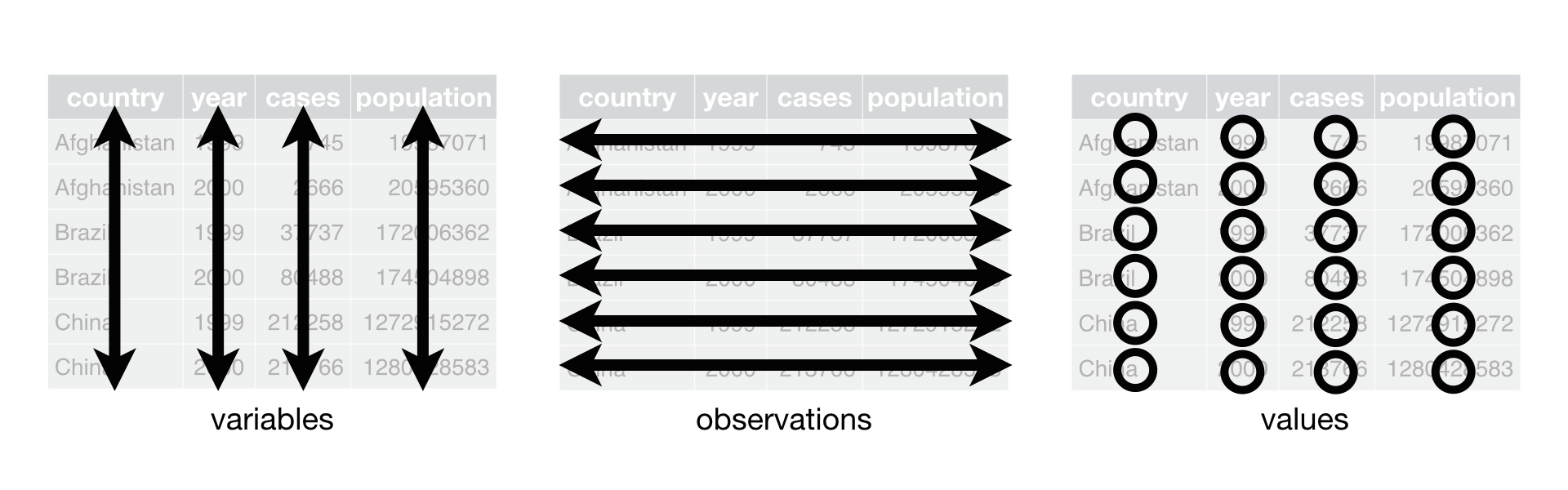
- Example table1 is tidy.

::: {.panel-tabset}

#### R

```{r}
table1
```
#### Python

```{python}
table1 = pd.DataFrame({
    'country': ['Afghanistan', 'Afghanistan', 'Brazil', 'Brazil', 'China', 'China'],
    'year': [1999, 2000, 1999, 2000, 1999, 2000],
    'cases': [745, 2666, 37737, 80488, 212258, 213766],
    'population': [19987071, 20595360, 172006362, 174504898, 1272915272, 1280428583]
})
table1
```

#### Julia

```{julia}
table1 = DataFrame(
    country = ["Afghanistan", "Afghanistan", "Brazil", "Brazil", "China", "China"],
    year = [1999, 2000, 1999, 2000, 1999, 2000],
    cases = [745, 2666, 37737, 80488, 212258, 213766],
    population = [19987071, 20595360, 172006362, 174504898, 1272915272, 1280428583]
)
```

:::


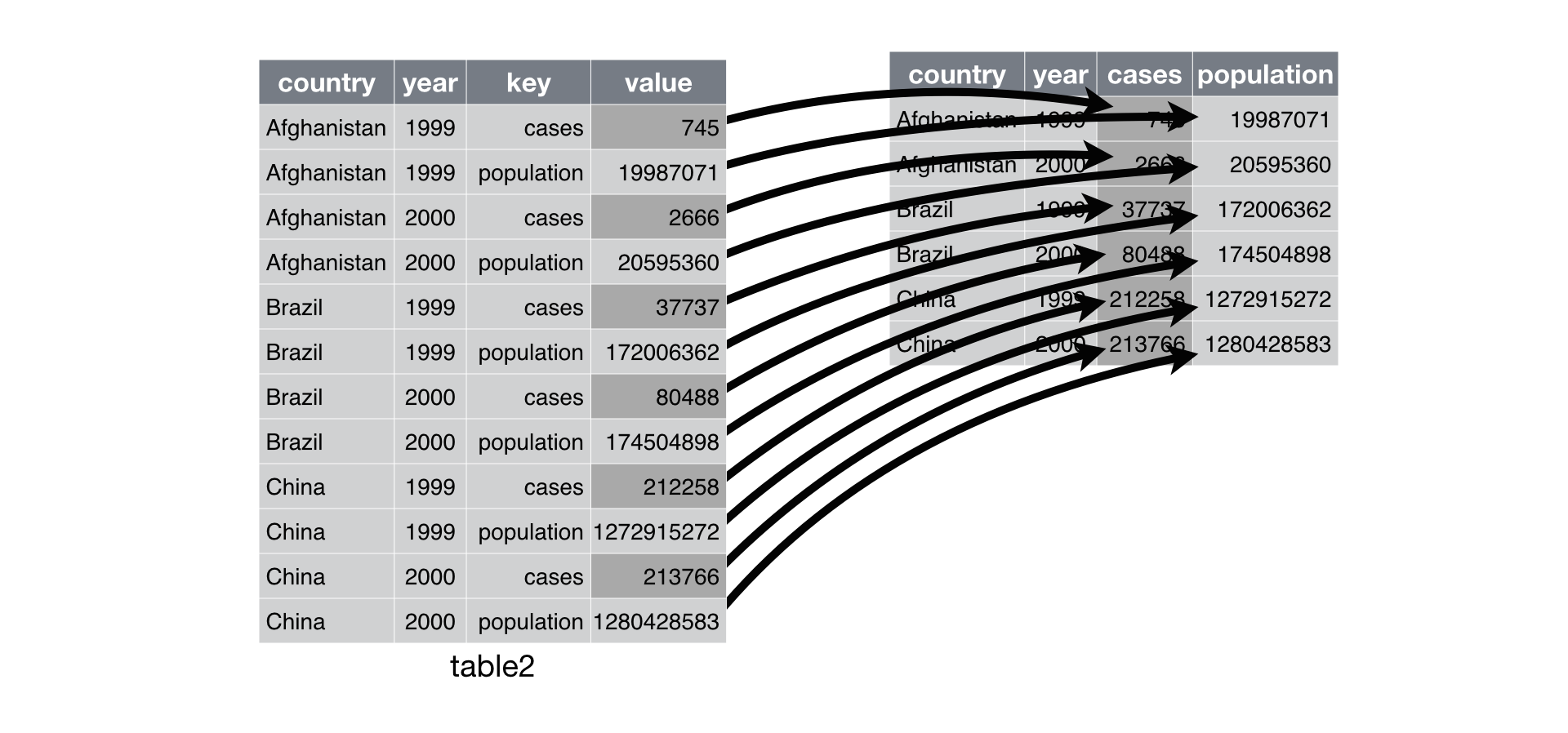
- Example table2 is not tidy (?). Actually this long format can be useful for plotting in ggplot2.

::: {.panel-tabset}

#### R

```{r}
table2
```

#### Python

```{python}
table2 = pd.DataFrame({
    'country': ['Afghanistan', 'Afghanistan', 'Afghanistan', 'Afghanistan', 'Brazil', 'Brazil', 'Brazil', 'Brazil', 'China', 'China', 'China', 'China'],
    'year': [1999, 1999, 2000, 2000, 1999, 1999, 2000, 2000, 1999, 1999, 2000, 2000,],
    'type': ['cases', 'population', 'cases', 'population', 'cases', 'population', 'cases', 'population', 'cases', 'population', 'cases', 'population'],
    'count': [745, 19987071, 2666, 20595360, 37737, 172006362, 80488, 174504898, 212258, 1272915272, 213766, 1280428583]
})
table2
```

#### Julia

```{julia}
table2 = DataFrame(
    country = ["Afghanistan", "Afghanistan", "Afghanistan", "Afghanistan", "Brazil", "Brazil", "Brazil", "Brazil", "China", "China", "China", "China"],
    year = [1999, 1999, 2000, 2000, 1999, 1999, 2000, 2000, 1999, 1999, 2000, 2000,],
    type = ["cases", "population", "cases", "population", "cases", "population", "cases", "population", "cases", "population", "cases", "population"],
    count = [745, 19987071, 2666, 20595360, 37737, 172006362, 80488, 174504898, 212258, 1272915272, 213766, 1280428583]
)
```

:::

- Example table3 is not tidy.

::: {.panel-tabset}

#### R

```{r}
table3
```

#### Python

```{python}
table3 = pd.DataFrame({
    'country': ['Afghanistan', 'Afghanistan', 'Brazil', 'Brazil', 'China', 'China'],
    'year': [1999, 2000, 1999, 2000, 1999, 2000],
    'rate': ['745/19987071', '2666/20595360', '37737/172006362', '80488/174504898', '212258/1272915272', '213766/1280428583']
})
table3
```

#### Julia

```{julia}
table3 = DataFrame(
    country = ["Afghanistan", "Afghanistan", "Brazil", "Brazil", "China", "China"],
    year = [1999, 2000, 1999, 2000, 1999, 2000],
    rate = ["745/19987071", "2666/20595360", "37737/172006362", "80488/174504898", "212258/1272915272", "213766/1280428583"]
)
```

:::

- table4a and table4b are not tidy.

::: {.panel-tabset}

#### R

```{r}
table4a
table4b
```

#### Python

```{python}
table4a = pd.DataFrame({
    'country': ['Afghanistan', 'Brazil', 'China'],
    '1999': [745, 37737, 212258],
    '2000': [2666, 80488, 213766]
})
table4a

table4b = pd.DataFrame({
    'country': ['Afghanistan', 'Brazil', 'China'],
    '1999': [19987071, 172006362, 1272915272],
    '2000': [20595360, 174504898, 1280428583]
})
table4b
```

#### Julia

```{julia}
table4a = DataFrame(
    country = ["Afghanistan", "Brazil", "China"],
    y1999 = [745, 37737, 212258],
    y2000 = [2666, 80488, 213766]
);
rename!(table4a, Dict(:y1999 => Symbol("1999"), :y2000 => Symbol("2000")))

table4b = DataFrame(
    country = ["Afghanistan", "Brazil", "China"],
    y1999 = [19987071, 172006362, 1272915272],
    y2000 = [20595360, 174504898, 1280428583]
);
rename!(table4b, Dict(:y1999 => Symbol("1999"), :y2000 => Symbol("2000")))
```

:::


### pivot_longer (gathering)

<p align="center">
<img src="./tidy-9.png" height="300">
</p>

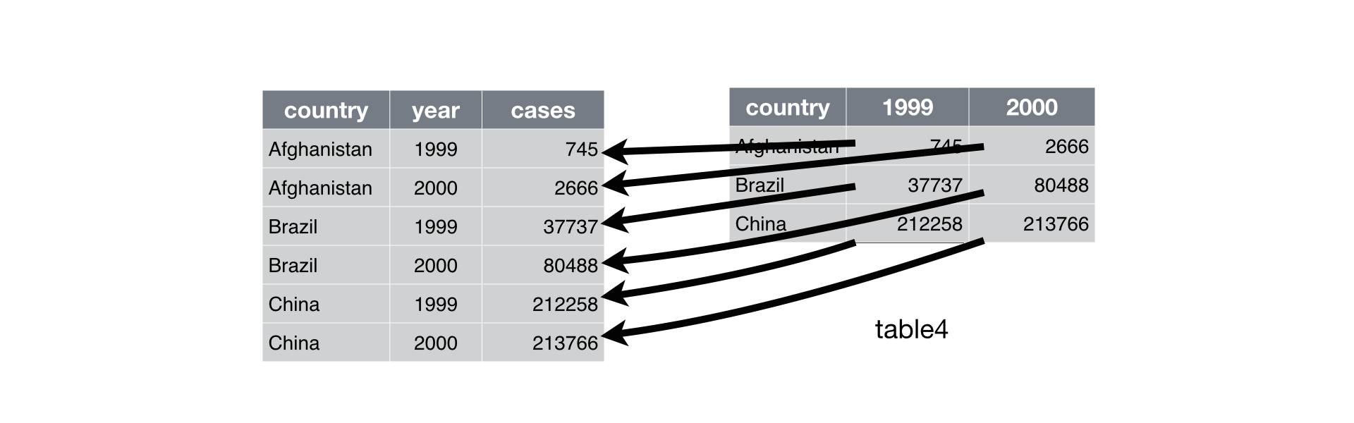
- `gather` (deprecated command) columns into a new pair of variables.
```{r}
# Deprecated command
table4a |>
  gather(`1999`, `2000`, key = "year", value = "cases")
```
    
- `gather` function has been superseded by `pivot_longer`.

- In Python, it's called `melt`. In Julia, it's called `stack`.

::: {.panel-tabset}

#### R

```{r}
table4a |>
  pivot_longer(c(`1999`, `2000`), names_to = "year", values_to = "cases")
```

#### Python

```{python}
tidy4a = table4a.melt(
  id_vars = ['country'],
  value_vars = ['1999', '2000'],
  var_name = 'year',
  value_name = 'cases'
)
tidy4a
```

#### Julia

```{julia}
tidy4a = @pipe stack(table4a, ["1999", "2000"]) |> 
  rename!(_, Dict(:variable => :year, :value => :cases))
```

:::

- We can gather table4b too and then join them

::: {.panel-tabset}

#### R

```{r}
tidy4a <- table4a |> 
  pivot_longer(c(`1999`, `2000`), names_to = "year", values_to = "cases")
# gather(`1999`, `2000`, key = "year", value = "cases")
tidy4b <- table4b |> 
  pivot_longer(c(`1999`, `2000`), names_to = "year", values_to = "population")
# gather(`1999`, `2000`, key = "year", value = "population")
left_join(tidy4a, tidy4b)
```

#### Python

```{python}
tidy4b = table4b.melt(
    id_vars = ['country'],
    value_vars = ['1999', '2000'],
    var_name = 'year',
    value_name = 'population'
    )
tidy4b

tidy4a.merge(
    tidy4b,
    on = ['country', 'year'],
    how = 'left'
    )
```

#### Julia


```{julia}
tidy4b = @pipe stack(table4b, ["1999", "2000"]) |> rename!(_, Dict(:variable => :year, :value => :population))
```

```{julia}
leftjoin!(tidy4a, tidy4b, on = [:country, :year])
```

:::

### pivot_wider (spreading)

<p align="center">
<img src="./tidy-8.png" height="300">
</p>

- Spreading is the opposite of gathering.
```{r}
table2 |>
  spread(key = type, value = count)
```

- `spread` function has been superseded by `pivot_wider`.

- In Python, it's called `pivot`. In Julia, it's called `unstack`.

::: {.panel-tabset}

#### R

```{r}
table2 |>
  pivot_wider(names_from = type, values_from = count)
```

#### Python

```{python}
table2.pivot(
    index = ['country', 'year'],
    columns = 'type',
    values = 'count'
)
```

#### Julia

```{julia}
unstack(table2, :type, :count)
```

:::

### Separating

<p align="center">
<img src="./tidy-17.png" height="300">
</p>

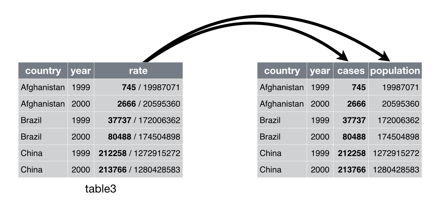
::: {.panel-tabset}

#### R

```{r}
# Before separation
table3
# After separation
table3 |> 
  separate(rate, into = c("cases", "population"))
```

- Separate into numeric values:
```{r}
table3 |> 
  separate(rate, into = c("cases", "population"), convert = TRUE)
```

- Separate at a fixed position:
```{r}
table3 |> 
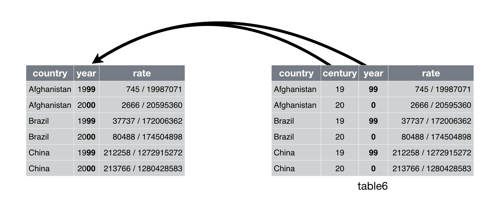
  separate(year, into = c("century", "year"), sep = 2)
```

#### Python

```{python}
# Before separation
table3
# After separation
table3[['cases', 'population']] = table3['rate'].apply(lambda x: pd.Series(str(x).split("/")))
table3
```

#### Julia

```{julia}
using SplitApplyCombine

# Before separation
table3
# After separation
insertcols!(table3, ([:cases, :population] .=> invert(split.(table3.rate, "/")))..., makeunique = true)
```

:::

### Unite

<p align="center">
<img src="./tidy-18.png" height="300">
</p>

::: {.panel-tabset}

#### R

```{r}
# Before unite
table5
```

- `unite()` is the inverse of `separate()`. 
```{r}
# After unite
table5 |> 
  unite(new, century, year, sep = "")
```

#### Python

```{python}
# Before unite
table5 = pd.DataFrame({
    'country': ['Afghanistan', 'Afghanistan', 'Brazil', 'Brazil', 'China', 'China'],
    'century': ['19', '20', '19', '20', '19', '20'],
    'year': ['99', '00', '99', '00', '99', '00'],
    'rate': ['745/19987071', '2666/20595360', '37737/172006362', '80488/174504898', '212258/1272915272', '213766/1280428583']
})
table5
```

```{python}
# After unite
table5['new'] = table5['century'] + table5['year']
table5
```

#### Julia

```{julia}
# Before unite
table5 = DataFrame(
    country = ["Afghanistan", "Afghanistan", "Brazil", "Brazil", "China", "China"],
    century = ["19", "20", "19", "20", "19", "20"],
    year = ["99", "00", "99", "00", "99", "00"],
    rate = ["745/19987071", "2666/20595360", "37737/172006362", "80488/174504898", "212258/1272915272", "213766/1280428583"]
)
# After unite
table5[!, :new] = parse.(Int, string.(table5[!, :century]) .* string.(table5[!, :year]));
table5
```

:::

### Drop missing values and/or duplicate rows

- Here's a tibble with some missing values and duplicated rows:

::: {.panel-tabset}

#### R

```{r}
df = tibble(
  country = c("Afghanistan", "Afghanistan", "Brazil", "China"),
  year = c(1999, 1999, 1999, NA),
  cases = c(745, 745, NA, 212258)
) |> print()
```

#### Python

```{python}
df = pd.DataFrame({
    'country': ["Afghanistan", "Afghanistan", "Brazil", "China"],
    'year': [1999, 1999, 1999, None],
    'cases': [745, 745, None, 212258]
})
df
```

#### Julia

```{julia}
df = DataFrame(
    country = ["Afghanistan", "Afghanistan", "Brazil", "China"],
    year = [1999, 1999, 1999, missing],
    cases = [745, 745, missing, 212258]
)
```

:::

- To drop all rows with missing values

::: {.panel-tabset}

#### R

```{r}
df |> drop_na()
```

#### Python

```{python}
df.dropna()
```

#### Julia

```{julia}
dropmissing(df)
```

:::

- To remove duplicate rows

::: {.panel-tabset}

#### R

```{r}
df |>
  distinct()
```

#### Python

```{python}
df.drop_duplicates()
```

#### Julia

```{julia}
unique(df)
```

:::


### Cheat sheet  

[Posit readr cheat sheet](https://rstudio.github.io/cheatsheets/html/tidyr.html) is extremely helpful. 

## Some practical decisions when ingesting data

- Are missing value parsed correctly? 

- Are data types parsed correctly? `chr` vs `fct`. data time. NA vs NaN.

- Are there any duplicated rows?

- Normalize variable/column names.

Example CSV data file:
```{bash}
head students.txt
```
Initial ingestion:
```{r}
read_csv("students.txt") |> 
  print(width = Inf)
```
Improved ingestion:
```{r}
read_csv(
  "students.txt", 
  na = c("N/A", ""),
  show_col_types = FALSE
  ) |> 
  # normalize variable name
  janitor::clean_names() |>
  # meal_plan: fct
  mutate(meal_plan = factor(meal_plan)) |>
  # parse age as integer
  mutate(age = parse_number(if_else(age == "five", "5", age))) |>
  print(width = Inf)
```