---
title: "Data Transformation With dplyr"
subtitle: Biostat 203B
author: "Dr. Hua Zhou @ UCLA"
date: today
format:
  html:
    theme: cosmo
    embed-resources: true
    number-sections: true
    toc: true
    toc-depth: 4
    toc-location: left
    code-fold: false
knitr:
  opts_chunk: 
    fig.align: 'center'
    fig.width: 6
    fig.height: 4
    message: FALSE
    cache: false
---

## Preamble

Display machine information for reproducibility.

::: {.panel-tabset}

#### R

```{r}
sessionInfo()
```

#### Python

```{python}
import IPython
print(IPython.sys_info())
```

#### Julia

```{julia}
using InteractiveUtils
versioninfo()
```

:::

Load tidyverse (R), Pandas (Python), and DataFrames.jl (Julia).

::: {.panel-tabset}

#### R

```{r}
library(tidyverse)
```

#### Python

```{python}
# Load the pandas library
import pandas as pd
# Load numpy for array manipulation
import numpy as np
```

#### Julia

```{julia}
using DataFrames, Pipe, StatsBase
```

:::

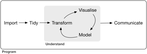
A typical data science project:

<p align="center">
<img src="./data-science.png" height="275">
</p>

## nycflights13 data

- Available from the nycflights13 package. 

- 336,776 flights that departed from New York City in 2013:

::: {.panel-tabset}

#### R

```{r}
library("nycflights13")
flights
```

#### Python

The nycflights13 data is available from the nycflights13 package in Python.
```{python}
from nycflights13 import flights

flights
```

Note there are some differences of this `flights` data from that in tidyverse. The data types for some variables are different. There are no natural ways in Pandas to hold integer column with missing values; so `dep_time` , `arr_time` are `float64` instead of `int64`. 
```{python}
flights.info()
```

To be more consistent with `nycflights13` in tidyverse, we cast `time_hour` to `datetime` type.
```{python}
flights['time_hour'] = pd.to_datetime(flights['time_hour'])
```

#### Julia

Let's use RCall.jl to retrieve the nycflights13 data from R.
```{julia}
using RCall

R"""
library(nycflights13)
"""

flights = rcopy(R"flights")
```

:::

To display more rows or columns: 

::: {.panel-tabset}

#### R

- By default, tibble prints the first 10 rows and all columns _that fit on screen_.

- To change number of rows and columns to display:
```{r}
nycflights13::flights |> 
  print(n = 10, width = Inf)
```
Here we see the **pipe operator** `|>` pipes the output from previous command to the (first) argument of the next command.

- To change the default print setting globally:
    - `options(tibble.print_max = n, tibble.print_min = m)`: if more than `m` rows, print only `n` rows.
    - `options(dplyr.print_min = Inf)`: print all row.
    - `options(tibble.width = Inf)`: print all columns.

#### Python

- Pandas by default displays 10 rows and limits the number of columns to the display area.

- We can override this behavior by
```{python}
#| eval: true
pd.set_option("display.max_rows", 500)
pd.set_option("display.max_columns", 20)
```


#### Julia

By default DataFrames.jl limits the number of rows and columns when displaying a data frame in a Jupyter Notebook to 25 and 100, respectively. You can override this behavior by changing the values of the `ENV["DATAFRAMES_COLUMNS"]` and `ENV["DATAFRAMES_ROWS"]` variables to hold the maximum number of columns and rows of the output. All columns or rows will be printed if those numbers are equal or lower than 0.

:::

## dplyr basics

* Pick observations (rows) by their values: `filter()`.

* Reorder the rows: `arrange()`.

* Pick variables (columns) by their names: `select()`.

* Create new variables with functions of existing variables: `mutate()`.

* Collapse many values down to a single summary: `summarise()`.

```
verb          meaning
--------------------------------------------
filter()      subset observations (or rows)
arrange()     re-order the observations
distinct()    remove duplicate entries
slice_*()     select rows by position
sample_*()    sample rows
--------------------------------------------
select()      select variables (or columns)
mutate()      add new variables (or columns)
relocate()    move variables (or columns) to new positions
rename()      rename variables (or columns)
--------------------------------------------
group_by()    aggregate
summarise()   reduce to a single row
--------------------------------------------
left_join()   merge two data objects
collect()     force computation and bring data back into R
```

## Manipulate rows (cases)

### Filter rows with `filter()`

- Flights on Jan 1st:

::: {.panel-tabset}

#### R

```{r}
# same as filter(flights, month == 1 & day == 1)
filter(flights, month == 1, day == 1)
```

#### Python

```{python}
flights[(flights['month'] == 1) & (flights['day'] == 1)]
```

#### Julia

```{julia}
filter(row -> (row.month == 1) & (row.day == 1), flights)
```

:::


- Flights in Nov or Dec:

::: {.panel-tabset}

#### R

```{r}
filter(flights, month == 11 | month == 12)
```

#### Python

```{python}
flights[(flights['month'] == 11) | (flights['month'] == 12)]
```

#### Julia

```{julia}
filter(row -> (row.month == 11) | (row.month == 12), flights)
```
:::

### Remove rows with duplicate values

- One row from each month:

::: {.panel-tabset}

#### R

```{r}
distinct(flights, month, .keep_all = TRUE)
```

- With `.keep_all = FALSE`, all variables/columns are kept:
```{r}
distinct(flights, month)
```

#### Python

```{python}
flights.drop_duplicates(subset = ['month'])
```

#### Julia

```{julia}
unique(flights, :month)
```

:::

### Sample rows

::: {.panel-tabset}

#### R

- Randomly select `n` rows:
```{r}
sample_n(flights, 10, replace = TRUE)
```

- Randomly select fraction of rows:
```{r}
sample_frac(flights, 0.1, replace = TRUE)
```

#### Python

Sample `n=10` rows.
```{python}
flights.sample(n = 10, axis = 0, replace = True)
```

Sample 10\% rows:
```{python}
flights.sample(frac = 0.1, replace = True)
```

#### Julia

I'm not sure whether there's a native function in DataFrames.jl for sampling.

Sample 10 rows:
```{julia}
rowidx = StatsBase.sample(1:nrow(flights), 10, replace = true);
flights[rowidx, :]
```
Sample 10\% rows:
```{julia}
rowidx = StatsBase.sample(
  1:nrow(flights), 
  round(Int, nrow(flights) * 0.1), 
  replace = true);
flights[rowidx, :]
```

:::


### Select rows by position

::: {.panel-tabset}

#### R

- Select rows by position:
```{r}
slice(flights, 1:5)
```

- First rows:
```{r}
slice_head(flights, n = 5)
```

- Last rows:
```{r}
slice_tail(flights, n = 5)
```

- Top `n` rows with the highest values:
```{r}
# deprecated: top_n(flights, 5, wt = time_hour)
# This function is quick
slice_max(flights, n = 5, order_by = time_hour) |>
  print(width = Inf)
```

- Bottom `n` rows with lowest values:
```{r}
# same as slice_max(flights, n = 5, order_by = desc(time_hour))
slice_min(flights, n = 5, order_by = time_hour) |>
  print(width = Inf)
```

- `slice_*` verbs apply to groups for grouped tibbles.

#### Python

- Select rows by position:
```{python}
flights.iloc[range(0, 5)]
```

- First rows:
```{python}
flights.head(5)
```

- Last rows:
```{python}
flights.tail(5)
```

- Top `n` rows with the highest values:
```{python}
flights.nlargest(n = 5, columns = 'time_hour')
```

- Bottom `n` rows with lowest values:
```{python}
flights.nsmallest(n = 5, columns = 'time_hour')
```
I don't think `nlargest` and `nsmallest` apply to grouped DataFrame. But I may be wrong.

#### Julia

- Select rows by position:
```{julia}
flights[1:5, :]
```

- First rows:
```{julia}
first(flights, 5)
```

- Last rows:
```{julia}
last(flights, 5)
```

- Top `n` rows with the highest values:
```{julia}
last(sort(flights, [:time_hour]), 5)
```

- Bottom `n` rows with lowest values:
```{julia}
first(sort(flights, [:time_hour]), 5)
```

:::

### Arrange rows with `arrange()`

::: {.panel-tabset}

#### R

- Sort in ascending order:
```{r}
arrange(flights, year, month, day)
```
Note input order matters!
```{r}
arrange(flights, day, month, year)
```

- Sort in descending order:
```{r}
arrange(flights, desc(arr_delay)) |>
  print(width = Inf)
```

- By default, `arrange` ignores grouping in grouped tibbles. Set `.by_group = TRUE` to arrange within each group.

```{r}
# What are the worst delays in each month?
flights |>
  group_by(month) |>
  arrange(desc(arr_delay), .by_group = TRUE) |>
  print(width = Inf)
```

#### Python

- Sort in ascending order:
```{python}
flights.sort_values(by = 'arr_delay')
```

- Sort in descending order:
```{python}
flights.sort_values(
  by = 'arr_delay',
  ascending = False
  )
```

- To sort within groups (`month`)
```{python}
flights.sort_values(
  by = ['month', 'arr_delay'],
  ascending = [True, False]
  )
```

#### Julia

Sort in ascending order:
```{julia}
sort(flights, [:arr_delay])
```

Sort in descending order:
```{julia}
sort(flights, [:arr_delay], rev = true)
```

To sort within groups (`month`):
```{julia}
sort(flights, [:month, order(:arr_delay, rev= true)])
```

:::

## Manipulate columns (variables)

### Select columns with `select()`

- Select columns by variable names:

::: {.panel-tabset}

#### R

```{r}
select(flights, year, month, day)
```

#### Python

```{python}
flights[['year', 'month', 'day']]
```

#### Julia

```{julia}
select(flights, [:year, :month, :day])
```

:::

- Pull values of _one_ column as a vector:

::: {.panel-tabset}

#### R

Not displayed because the vector is long.
```{r}
#| eval: false
pull(flights, year)
```

#### Python

```{python}
#| eval: false
# Following are same
flights.year
flights.loc[:, 'year']
```
#### Julia

```{julia}
#| eval: false
# Return a vector
flights.year
# Return a vector
flights."year"
# Return a vector
flights[!, :year] # does not make a copy
# Return a vector
flights[!, "year"] # does not make a copy
# Return a vector
flights[:, :year] # make a copy!
# Return a vector
flights[:, "year"] # make a copy!
```

:::

- Select columns between two variables:

::: {.panel-tabset}

#### R

```{r}
select(flights, year:day)
```

#### Python

```{python}
flights.loc[:, 'year':'day']
```

#### Julia

```{julia}
select(flights, Between(:year, :day))
```

:::

- Select all columns _except_ those between two variables:

::: {.panel-tabset}

#### R

```{r}
select(flights, -(year:day))
```

#### Python

```{python}
flights.drop(flights.loc[:, 'year':'day'].columns, axis = 1)
```

#### Julia

```{julia}
select(flights, Not(Between(:year, :day)))
```

:::

- Select columns by positions:

::: {.panel-tabset}

#### R

```{r}
select(flights, seq(1, 10, by = 2))
```

#### Python

```{python}
flights.iloc[:, range(0, 9, 2)]
```

#### Julia

```{julia}
select(flights, 1:2:10)
```

:::

- Move variables to the start of data frame:

::: {.panel-tabset}

#### R

```{r}
select(flights, time_hour, air_time, everything())
```
 
#### Python (???)

Not sure what's the optimal way to do this.
```{python}
# Note time_hour is missing in Python dataframe
cols_to_move = ['arr_delay', 'air_time']
flights[cols_to_move + [x for x in flights.columns if x not in cols_to_move]]
```

#### Julia

```{julia}
select(flights, :time_hour, :air_time, Not([:time_hour, :air_time]))
```

:::
 
- Helper functions in `dplyr`.

    * `everying()`: matches all variables.
    
    * `last_col()`: select last variable, possibly with an offset.

    * `starts_with("abc")`: matches names that begin with “abc”.

    * `ends_with("xyz")`: matches names that end with “xyz”.

    * `contains("ijk")`: matches names that contain “ijk”.

    * `matches("(.)\\1")`: selects variables that match a regular expression.

    * `num_range("x", 1:3)`: matches x1, x2 and x3.
    
    * `all_of()`: matches variables names in a character vector. All names must be present, otherwise an out-of-bounds error is thrown.
    
    * `any_of()`: same as `all_of()`, but no error is thrown.

### Add new variables with `mutate()`

- A tibble with fewer columns.

::: {.panel-tabset}

#### R

```{r}
flights_sml <- 
  select(flights, year:day, ends_with("delay"), distance, air_time)
flights_sml
```

#### Python (???)

Is there better way?
```{python}
import re

cols = ['year', 'month', 'day'] + list(filter(re.compile(".*delay").match, flights.columns)) + ['distance', 'air_time']
flights_sml = flights.loc[:, cols]
flights_sml
```

#### Julia

```{julia}
flights_sml = select(flights, Between(:year, :day), r".*delay$", :distance, :air_time)
flights_sml
```

:::

- Add variables `gain` and `speed`:

::: {.panel-tabset}

#### R

```{r}
mutate(
  flights_sml,
  gain = arr_delay - dep_delay,
  speed = distance / air_time * 60
)
```

#### Python

```{python}
flights_sml['gain'] = flights_sml['arr_delay'] - flights_sml['dep_delay']
flights_sml['speed'] = flights_sml['distance'] / flights_sml['air_time'] * 60
flights_sml
```

#### Julia

Julia analog is `transform`:
```{julia}
# Following are equivalent
transform(flights_sml, [:arr_delay, :dep_delay] => (-) => :gain)
insertcols!(flights_sml, :gain => flights.arr_delay - flights.dep_delay)
```

:::

- Refer to columns that you’ve just created:

::: {.panel-tabset}

#### R

```{r}
mutate(flights_sml,
       gain = arr_delay - dep_delay,
       hours = air_time / 60,
       gain_per_hour = gain / hours
)
```

#### Python (???)

Not sure how to refer to columns in the same command.

#### Julia (???)

Not sure how to do this, except using two lines.
```{julia}
# Following are equivalent
@pipe flights |> 
  transform(
    _ , 
    [:arr_delay, :dep_delay] => (-) => :gain,
    [:air_time] => (x -> x / 60)  => :hours,
  ) |> 
  transform(
    _,
    [:gain, :hours] => ByRow(/) => :gain_per_hour
  )
```

:::

- Only keep the new variables by `transmute()`:
```{r}
transmute(
  flights,
  gain = arr_delay - dep_delay,
  hours = air_time / 60,
  gain_per_hour = gain / hours
)
```

- `mutate_all()`: apply funs to all columns.

::: {.panel-tabset}

#### R

```{r}
#| eval: false
mutate_all(data, funs(log(.), log2(.)))
```

#### Python (???)

TODO

#### Julia

```{julia}
#| eval: false
mapcols(col -> 2col, df)
```

:::

- `mutate_at()`: apply funs to specific columns.
```{r}
#| eval: false
mutate_at(data, vars(-Species), funs(log(.)))
```

- `mutate_if()`: apply funs of one type
```{r}
#| eval: false
mutate_if(data, is.numeric, funs(log(.)))
```

## Summaries

### Summaries with `summarise()`

- Mean of a variable:

::: {.panel-tabset}

#### R

```{r}
summarise(flights, delay = mean(dep_delay, na.rm = TRUE))
```

#### Python

```{python}
flights.agg({'dep_delay': np.mean})
```

#### Julia

```{julia}
combine(flights, :dep_delay => (x -> mean(skipmissing(x))) => :delay)
```

:::
 
- Convert a tibble into a grouped tibble:

::: {.panel-tabset}

#### R

```{r}
by_day <- group_by(flights, year, month, day) |>
  print(width = Inf)
```

#### Python

```{python}
by_day = flights.groupby(['year', 'month', 'day'])
by_day
```

#### Julia

```{julia}
by_day = groupby(flights, [:year, :month, :day])
by_day
```

:::


- Grouped summaries:
```{r}
summarise(by_day, delay = mean(dep_delay, na.rm = TRUE))
```

### Pipe

- Consider following analysis (find destinations excluding `HNL` that have >20 flights, and calculate the average distances and arrival delay):
```{r}
#| message: false
by_dest <- group_by(flights, dest)
delay <- summarise(by_dest, count = n(),
                   dist = mean(distance, na.rm = TRUE),
                   delay = mean(arr_delay, na.rm = TRUE)
)
delay <- filter(delay, count > 20, dest != "HNL")
delay
```

----

- Cleaner code using pipe `|>`:
```{r}
delays <- flights |> 
  group_by(dest) |> 
  summarise(
    count = n(),
    dist = mean(distance, na.rm = TRUE),
    delay = mean(arr_delay, na.rm = TRUE)
  ) |> 
  filter(count > 20, dest != "HNL")
delays
```

- ggplot2 accepts pipe too.

```{r}
delays |>
  ggplot(mapping = aes(x = dist, y = delay)) +
  geom_point(aes(size = count), alpha = 1/3) + 
  geom_smooth(se = FALSE) + 
  labs(x = "Distance from NYC (miles)",
       y = "Arrival delay (mins)")
```

### Other summary functions

- Location: `mean(x)`, `median(x)`.

::: {.panel-tabset}

#### R

```{r}
# Equivalent code using filter
# not_cancelled <- flights |> 
#   filter(!is.na(dep_delay), !is.na(arr_delay)) |>
#   print(width = Inf)
not_cancelled <- flights |>
  drop_na(dep_delay, arr_delay) |>
  print(width = Inf)
```
```{r}
not_cancelled |> 
  group_by(year, month, day) |> 
  summarise(
    avg_delay1 = mean(arr_delay),
    avg_delay2 = mean(arr_delay[arr_delay > 0]), # the average positive delay
  )
```
Question: why is the `day` group dropped?

#### Python

```{python}
not_cancelled = flights.dropna(subset = ['dep_delay', 'arr_delay'])
not_cancelled
```

```{python}
flights.groupby(['year', 'month', 'day']).agg(
  avg_delay1 = ('arr_delay', np.mean), 
  avg_delay2 = ('arr_delay', lambda x: np.mean(x[x > 0]))
)
```

#### Julia

```{julia}
not_cancelled = dropmissing(flights, [:dep_delay, :arr_delay])
not_cancelled
```

```{julia}
@pipe not_cancelled |>
  groupby(_, [:year, :month, :day]) |> 
  combine(
    _, 
    :arr_delay => (x -> [(mean(x), mean(skipmissing(x[x .>= 0])))]) => [:avg_delay1, :avg_delay2]
    )
```

:::

- Spread: `sd(x)`, `IQR(x)`, `mad(x)`.

::: {.panel-tabset}

#### R

```{r}
# destinations with largest variation in distance
not_cancelled |> 
  group_by(dest) |> 
  summarise(distance_sd = sd(distance)) |> 
  arrange(desc(distance_sd))
```

#### Python

```{python}
flights.groupby(['dest']).agg(
  distance_sd = ('distance', np.std)
).sort_values('distance_sd', ascending = False)
```

#### Julia

```{julia}
@pipe flights |>
  groupby(_, :dest) |>
  combine(_, :distance => std => :distance_sd) |>
  sort(_, :distance_sd, rev = true)
```

:::
    
- Rank: `min(x)`, `quantile(x, 0.25)`, `max(x)`.

::: {.panel-tabset}

#### R

```{r}
# Earliest and latest flights on each day?
not_cancelled |> 
  group_by(year, month, day) |> 
  summarise(
    first = min(dep_time),
    last = max(dep_time)
  )
```

#### Python

```{python}
not_cancelled.groupby(['year', 'month', 'day']).agg(
  first = ('dep_time', np.min),
  last = ('dep_time', np.max)
)
```

#### Julia

```{julia}
@pipe not_cancelled |>
  groupby(_, [:year, :month, :day]) |>
  combine(_, :dep_time => (x -> [extrema(x)]) => [:first, :last])
```

:::

- Position: `first(x)`, `nth(x, 2)`, `last(x)`. Note unless the variable is sorted, `first` is different from `min` and `last` is different from `max`.

::: {.panel-tabset}

#### R

```{r}
not_cancelled |> 
  group_by(year, month, day) |> 
  summarise(
    first_dep = first(dep_time), 
    last_dep = last(dep_time)
  )
```

#### Python

```{python}
not_cancelled.groupby(['year', 'month', 'day']).agg(
  first_dep = ('dep_time', lambda x: x.iloc[0]),
  last_dep = ('dep_time', lambda x: x.iloc[-1]),
)
```

#### Julia

```{julia}
@pipe not_cancelled |>
  groupby(_, [:year, :month, :day]) |>
  combine(
    _, 
    :dep_time => first => :first_dep,
    :dep_time => last => :last_dep
    )
```

:::

- Count: `n(x)`, `sum(!is.na(x))`, `n_distinct(x)`.

::: {.panel-tabset}

#### R

```{r}
# Which destinations have the most carriers?
not_cancelled |> 
  group_by(dest) |> 
  summarise(carriers = n_distinct(carrier)) |> 
  arrange(desc(carriers))
```

Similarly
```{r}
# which destination has most flights from NYC?
not_cancelled |> 
  count(dest) |>
  arrange(desc(n))
```

#### Python

```{python}
not_cancelled.groupby('dest').agg(
  carriers = ('carrier', lambda x: x.nunique(dropna = True))
).sort_values('carriers', ascending = False)
```

#### Julia

```{julia}
@pipe not_cancelled |>
  groupby(_, :dest) |>
  combine(_, :carrier => length ∘ unique => :carriers) |>
  sort(_, :carriers, rev = true)
```

:::

- Example: which aircraft flew most (in distance) in 2013?

::: {.panel-tabset}

#### R

```{r}
not_cancelled |> 
  count(tailnum, wt = distance) |>
  arrange(desc(n))
```

#### Python

```{python}
not_cancelled.groupby('tailnum').agg(
  total_distance = ('distance', sum)
).sort_values('total_distance', ascending = False)
```

#### Julia

```{julia}
@pipe not_cancelled |>
  groupby(_, :tailnum) |>
  combine(_, :distance => sum ∘ skipmissing => :total_distance) |>
  sort(_, :total_distance, rev = true)
```

:::

- Example: How many flights left before 5am? (these usually indicate delayed flights from the previous day)

::: {.panel-tabset}

#### R

```{r}
not_cancelled |> 
  group_by(year, month, day) |> 
  summarise(n_early = sum(dep_time < 500)) |>
  arrange(desc(n_early))
```

#### Python

```{python}
not_cancelled.groupby(['year', 'month', 'day']).agg(
  n_early = ('dep_time', lambda x: sum(x < 500))
).sort_values('n_early', ascending = False)
```

#### Julia

```{julia}
@pipe not_cancelled |>
  groupby(_, [:year, :month, :day]) |>
  combine(_, :dep_time => (x -> sum(skipmissing(x .< 500))) => :n_early) |>
  sort(_, :n_early, rev = true)
```

:::

- Example: What proportion of flights are delayed by more than an hour?

::: {.panel-tabset}

#### R

```{r}
not_cancelled |> 
  group_by(year, month, day) |> 
  summarise(hour_perc = mean(arr_delay > 60)) |>
  arrange(desc(hour_perc))
```

#### Python

```{python}
not_cancelled.groupby(['year', 'month', 'day']).agg(
  hour_perc = ('arr_delay', lambda x: np.mean(x > 60))
).sort_values('hour_perc', ascending = False)
```

#### Julia

```{julia}
@pipe not_cancelled |>
  groupby(_, [:year, :month, :day]) |>
  combine(_, :arr_delay => (x -> mean(skipmissing(x .> 60))) => :hour_perc) |>
  sort(_, :hour_perc, rev = true)
```

:::

## Grouped mutates (and filters)

- Recall the `flights_sml` tibble created earlier:

::: {.panel-tabset}

#### R

```{r}
flights_sml
```

#### Python

```{python}
flights_sml
```

#### Julia

```{julia}
flights_sml
```

:::

- Find the worst members of each group:

::: {.panel-tabset}

#### R

```{r}
flights_sml |> 
  group_by(year, month, day) |>
  filter(rank(desc(arr_delay)) < 10)
```

#### Python

```{python}
flights_sml.groupby(
  ['year', 'month', 'day']
  )['arr_delay'].nlargest(
    n = 10
)
```

#### Julia

```{julia}
@pipe flights_sml |>
  dropmissing(_, :arr_delay) |>
  groupby(_, [:year, :month, :day]) |>
  combine(
    _,
    :arr_delay => (x -> x[x .>= partialsort(x, 10, rev = true)])
    )
```

:::

- Find all groups bigger than a threshold:

::: {.panel-tabset}

#### R

```{r}
popular_dests <- flights |> 
  group_by(dest) |> 
  filter(n() > 365) |>
  print(width = Inf)
```

#### Python

```{python}
popular_dests = flights.groupby('dest').filter(lambda x: len(x) > 365)
popular_dests
```

#### Julia

```{julia}
popular_dests = @pipe flights |> 
  groupby(_, :dest) |>
  combine(_) do sdf
    nrow(sdf) > 365 ? sdf : DataFrame()
  end
popular_dests
```

:::

- Standardise to compute per group metrics:

::: {.panel-tabset}

#### R

```{r}
popular_dests <- popular_dests |> 
  filter(arr_delay > 0) |>
  mutate(prop_delay = arr_delay / sum(arr_delay)) |>
  select(year:day, dest, arr_delay, prop_delay) |>
  print(width = Inf)
```

#### Python

```{python}
popular_dests[popular_dests['arr_delay'] > 0].groupby(
  'dest'
  ).apply(
  lambda x: x['arr_delay'] / x['arr_delay'].sum()
)
```

#### Julia

```{julia}
@pipe popular_dests |> 
  dropmissing(_, :arr_delay) |>
  subset(_, :arr_delay => x -> x .> 0 ) |>
  groupby(_, :dest) |>
  combine(_, :arr_delay => (x -> x ./ sum(x)) => :prop_delay)
```

:::

## Combine tables

nycflights13 package has >1 tables:

- We already know a lot about flights:

::: {.panel-tabset}

#### R

```{r}
flights |> print(width = Inf)
```

#### Python

```{python}
flights
```

#### Julia

```{julia}
flights
```

:::


- airlines:

::: {.panel-tabset}

#### R

```{r}
airlines
```

#### Python

```{python}
from nycflights13 import airlines

airlines
```
#### Julia

```{julia}
airlines = rcopy(R"airlines")
```

:::

- airports:

::: {.panel-tabset}

#### R

```{r}
airports
```

#### Python

```{python}
from nycflights13 import airports

airports
```

#### Julia

```{julia}
airports = rcopy(R"airports")
```

:::

- planes:

::: {.panel-tabset}

#### R

```{r}
planes
```

#### Python

```{python}
from nycflights13 import planes

planes
```

#### Julia

```{julia}
planes = rcopy(R"planes")
```

:::


- Weather:

::: {.panel-tabset}

#### R

```{r}
weather |>
  print(width = Inf)
```

#### Python

```{python}
from nycflights13 import weather

weather
```

#### Julia

```{julia}
weather = rcopy(R"weather")
```

:::


## Relational data

<p align="center">
<img src="./relational-nycflights.png" height="375">
</p>

For the MIMIC-III data, the relation structure can be explored at <https://mit-lcp.github.io/mimic-schema-spy/relationships.html>.

### Keys

- A **primary key** uniquely identifies an observation in its own table.

- A **foreign key** uniquely identifies an observation in another table.

## Combine variables (columns)

### Demo tables

::: {.panel-tabset}

#### R

```{r}
(x <- tribble(
  ~key, ~val_x,
  1, "x1",
  2, "x2",
  3, "x3"
))
```
```{r}
(y <- tribble(
  ~key, ~val_y,
  1, "y1",
  2, "y2",
  4, "y3"
))
```

#### Python

```{python}
x = pd.DataFrame({
  'key': [1, 2, 4],
  'val_x': ['x1', 'x2', 'x3']
})
x
```
```{python}
y = pd.DataFrame({
  'key': [1, 2, 3],
  'val_y': ['y1', 'y2', 'y3']
})
x
```
#### Julia

```{julia}
x = DataFrame(
  key = 1:3,
  val_x = ["x1", "x2", "x3"]
)
y = DataFrame(
  key = [1, 2, 4],
  val_y = ["y1", "y2", "y3"]
)
```

:::

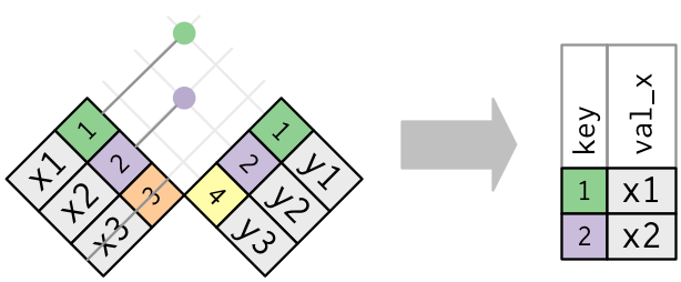
### Inner join

- An **inner join** matches pairs of observations whenever their keys are equal:

<p align="center">
<img src="./join-inner.png" height="150">
</p>


::: {.panel-tabset}

#### R

```{r}
inner_join(x, y, by = "key")
```
Same as
```{r}
#| eval: false
x |> inner_join(y, by = "key")
```

#### Python

```{python}
x.join(y.set_index('key'), on = 'key', how = 'inner')
```

#### Julia

```{julia}
innerjoin(x, y, on = :key)
```

:::

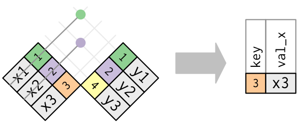
### Outer join

- An **outer join** keeps observations that appear in at least one of the tables. 

- Three types of outer joins: left join, right join, and full join.

- A **left join** keeps all observations in `x`.
    
::: {.panel-tabset}    

#### R
  
```{r}
left_join(x, y, by = "key")
```

#### Python

```{python}
x.join(y.set_index('key'), on = 'key', how = 'left')
```

#### Julia

```{julia}
leftjoin(x, y, on = :key)
```

:::
    
- A **right join** keeps all observations in `y`.
    
::: {.panel-tabset}    

#### R
    
```{r}
right_join(x, y, by = "key")
```

#### Python

```{python}
x.join(y.set_index('key'), on = 'key', how = 'right')
```

#### Julia

```{julia}
rightjoin(x, y, on = :key)
```

:::
    
- A **full join** keeps all observations in `x` or `y`.
    
::: {.panel-tabset}

#### R
    
```{r}
full_join(x, y, by = "key")
```

#### Python

```{python}
x.join(y.set_index('key'), on = 'key', how = 'outer')
```

#### Julia

```{julia}
outerjoin(x, y, on = :key)
```

:::
    
<p align="center">
<img src="./join-outer.png" width="50%">
</p>
    
### Duplicate keys

- One table has duplicate keys.

    <p align="center">
    <img src="./join-one-to-many.png" height="200">
    </p>

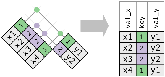
::: {.panel-tabset}

#### R

```{r}
x <- tribble(
  ~key, ~val_x,
  1, "x1",
  2, "x2",
  2, "x3",
  1, "x4"
)
x
y <- tribble(
  ~key, ~val_y,
  1, "y1",
  2, "y2"
)
y
left_join(x, y, by = "key")
```

#### Python

```{python}
x = pd.DataFrame({
  'key': [1, 2, 2, 1],
  'val_x': ["x1", "x2", "x3", "x4"]
})
x
y = pd.DataFrame({
  'key': [1, 2],
  'val_y': ["y1", "y2"]
})
y
x.join(y.set_index('key'), on = 'key', how = 'left')
```

#### Julia

```{julia}
x = DataFrame(
  key = [1, 2, 2, 1],
  val_x = ["x1", "x2", "x3", "x4"]
)
y = DataFrame(
  key = [1, 2],
  val_y = ["y1", "y2"]
)
leftjoin(x, y, on = :key)
```

:::

- Both tables have duplicate keys. You get all possible combinations, the Cartesian product:

    <p align="center">
    <img src="./join-many-to-many.png" height="250">
    </p>

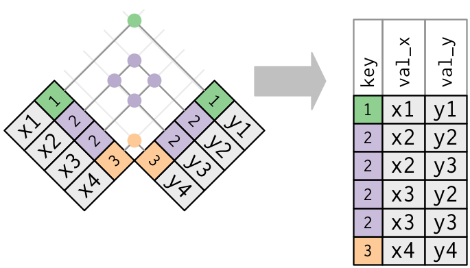
::: {.panel-tabset}

#### R

```{r}
x <- tribble(
  ~key, ~val_x,
  1, "x1",
  2, "x2",
  2, "x3",
  3, "x4"
)
y <- tribble(
  ~key, ~val_y,
  1, "y1",
  2, "y2",
  2, "y3",
  3, "y4"
)
left_join(x, y, by = "key")
```

#### Python

```{python}
x = pd.DataFrame({
  'key': [1, 2, 2, 3],
  'val_x': ["x1", "x2", "x3", "x4"]
})
x
y = pd.DataFrame({
  'key': [1, 2, 2, 3],
  'val_y': ["y1", "y2", "y3", "y4"]
})
y
x.join(y.set_index('key'), on = 'key', how = 'left')
```

#### Julia

```{julia}
x = DataFrame(
  key = [1, 2, 2, 3],
  val_x = ["x1", "x2", "x3", "x4"]
)
y = DataFrame(
  key = [1, 2, 2, 3],
  val_y = ["y1", "y2", "y3", "y4"]
)
leftjoin(x, y, on = :key)
```

:::

- Let's create a narrower table from the flights data:

::: {.panel-tabset}

#### R

```{r}
flights2 <- flights |> 
  select(year:day, hour, origin, dest, tailnum, carrier) |>
  print(width = Inf)
```

#### Python

```{python}
flights2 = flights[['year', 'month', 'day', 'hour', 'origin', 'dest', 'tailnum', 'carrier']]
flights2
```

#### Julia

```{julia}
flights2 = select(
  flights, 
  Between(:year, :day), 
  :hour, 
  :origin, 
  :dest, 
  :tailnum, 
  :carrier
  )
```

:::

- We want to merge with the `weather` table:

::: {.panel-tabset}

#### R

```{r}
weather
```

#### Python

```{python}
weather
```

#### Julia

```{julia}
weather
```

:::

### Defining the key columns

::: {.panel-tabset}

#### R

- `by = NULL` (default): use all variables that appear in both tables:
```{r}
# same as: flights2 |> left_join(weather)
left_join(flights2, weather)
```

- `by = "x"`: use the common variable `x`:
```{r}
# same as: flights2 |> left_join(weather)
left_join(flights2, planes, by = "tailnum")
```

- `by = c("a" = "b")`: match variable `a` in table `x` to the variable `b` in table `y`.
```{r}
# same as: flights2 |> left_join(weather)
left_join(flights2, airports, by = c("dest" = "faa"))
```

#### Python

- Match multiple keys using multi-index:
```{python}
keys = ['origin', 'year', 'month', 'day', 'hour']
flights2.join(
  weather.set_index(keys),
  on = keys,
  how = 'left')
```

- Match the common variable `tailnum`:
```{python}
flights2.join(
  planes.set_index('tailnum'), 
  on = 'tailnum', 
  how = 'left',
  lsuffix = '_x',
  rsuffix = '_y'
  )
```

- Match variable `a` in table `x` to the variable `b` in table `y`.
```{python}
flights2.set_index(
  'dest'
  ).join(
    airports.set_index('faa'), 
    how = 'left'
    )
```

#### Julia

- Match multiple variables:
```{julia}
leftjoin(
  flights2, 
  weather, 
  on = [:year, :month, :day, :hour, :origin]
  )
```

- Match the common variable `tailnum`:
```{julia}
leftjoin(
  flights2, 
  planes, 
  on = :tailnum,
  makeunique = true,
  matchmissing = :notequal
  )
```

- Match variable `a` in table `x` to the variable `b` in table `y`.
```{julia}
leftjoin(
  flights2,
  airports,
  on = :dest => :faa
  )
```

:::

## Combine cases (rows)

- Top 10 most popular destinations:

::: {.panel-tabset}

#### R

```{r}
top_dest <- flights |>
  count(dest, sort = TRUE) |>
  head(10) |>
  print()
```

#### Python

```{python}
top_dest = flights.groupby('dest')['dest'].count(
  ).to_frame(
    name = 'n'
    ).reset_index(
      ).sort_values(
        'n', 
        ascending = False
        ).head(10)
top_dest      
```

#### Julia

```{julia}
top_dest = @pipe flights |> 
  groupby(_, :dest) |>
  combine(_, nrow) |>
  sort(_, :nrow, rev = true) |>
  first(_, 10)
```

:::


- How to filter the cases that fly to these destinations?     
    
### Semi-join

- `semi_join(x, y)` keeps the rows in `x` that have a match in `y`.

    <p align="center">
    <img src="./join-semi.png" height="200">
    </p>

::: {.panel-tabset}

#### R

```{r}
semi_join(flights, top_dest)
```

#### Python

```{python}
flights.loc[flights['dest'].isin(top_dest['dest'])]
```

#### Julia

```{julia}
semijoin(flights, top_dest, on = :dest)
```

:::

### Anti-join

- `anti_join(x, y)` keeps the rows that don’t have a match.

    <p align="center">
    <img src="./join-anti.png" height="200">
    </p>

- Useful to see what will not be joined.


::: {.panel-tabset}

#### R

```{r}
# Planes that are not in planes table
flights |> 
  anti_join(planes, by = "tailnum") |>
  count(tailnum, sort = TRUE)
```
#### Python

```{python}
flights.loc[-flights['tailnum'].isin(planes['tailnum'])].groupby('tailnum')['tailnum'].count().sort_values(ascending = False)
```

#### Julia

```{julia}
@pipe antijoin(
  flights, 
  planes, 
  on = :tailnum, 
  matchmissing = :notequal
  ) |>
  groupby(_, :tailnum) |>
  combine(_, nrow) |>
  sort(_, :nrow, rev = true)
```

:::


## Set operations

- Generate two tables:

::: {.panel-tabset}

#### R

```{r}
(df1 <- tribble(
  ~x, ~y,
  1,  1,
  2,  1
))
```
```{r}
(df2 <- tribble(
  ~x, ~y,
  1,  1,
  1,  2
))
```

#### Python

```{python}
df1 = pd.DataFrame({
  'x': [1, 2],
  'y': [1, 1]
})
df1
df2 = pd.DataFrame({
  'x': [1, 1],
  'y': [1, 2]
})
df2
```

#### Julia

```{julia}
df1 = DataFrame(
  x = [1, 2],
  y = [1, 1]
)
df2 = DataFrame(
  x = [1, 1],
  y = [1, 2]
)
```

:::


- `bind_rows(x, y)` stacks table `x` one on top of `y`. 

::: {.panel-tabset}

#### R

```{r}
bind_rows(df1, df2)
```

#### Python

```{python}
pd.concat([df1, df2], axis = 0)
```

#### Julia

```{julia}
vcat(df1, df2)
```

:::


- `intersect(x, y)` returns rows that appear in both `x` and `y`.

::: {.panel-tabset}

#### R

```{r}
intersect(df1, df2)
```

#### Python

```{python}
pd.merge(df1, df2, how = 'inner', on = ['x', 'y'])
```

#### Julia

```{julia}
DataFrame(intersect(eachrow(df1), eachrow(df2)))
```

:::

- `union(x, y)` returns unique observations in `x` and `y`.

::: {.panel-tabset}

#### R

```{r}
union(df1, df2)
```

#### Python

```{python}
pd.merge(df1, df2, how = 'outer', on = ['x', 'y'])
```

#### Julia

```{julia}
DataFrame(union(eachrow(df1), eachrow(df2)))
```

:::


- `setdiff(x, y)` returns rows that appear in `x` but not in `y`.

::: {.panel-tabset}

#### R

```{r}
setdiff(df1, df2)
```
```{r}
setdiff(df2, df1)
```

#### Python (???)

Not sure how to do this elegantly.

#### Julia

```{julia}
DataFrame(setdiff(eachrow(df1), eachrow(df2)))
DataFrame(setdiff(eachrow(df2), eachrow(df1)))
```

:::


## Cheat sheet  

[Posit dplyr cheat sheet](https://rstudio.github.io/cheatsheets/html/data-transformation.html) is extremely helpful.