{width=500px height=400px}
{width=500px height=200px}
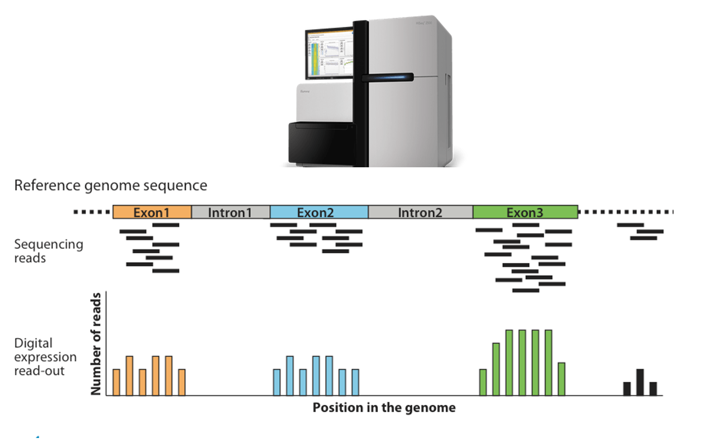
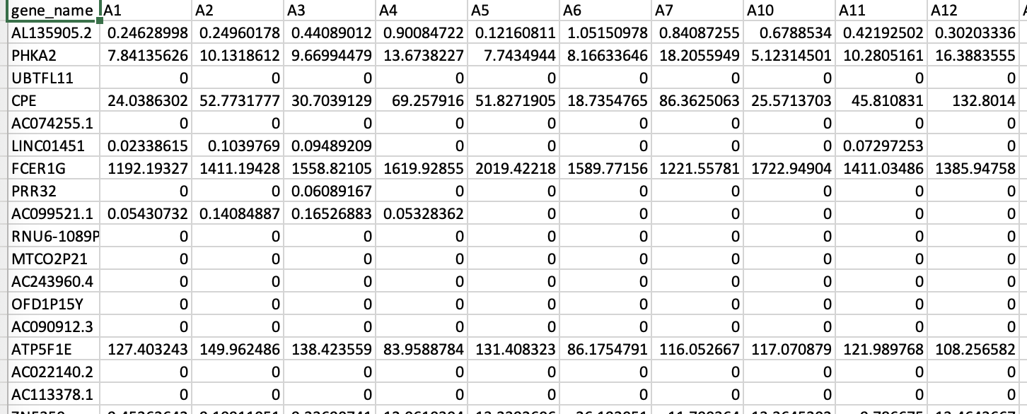
- 183 lung transplant recipients with 58,735 gene transcripts' expression levels measured
)
{width=700px height=200px}
{width=500px height=600px}
### Example: handwritten digit recognition
::: {#fig-handwritten-digits}
{width=500px height=300px}
{width=500px height=300px}
Examples of handwritten digits from the MNIST corpus (ISL Figure 10.3).
:::
- Input: 784 pixel values from $28 \times 28$ grayscale images. Output: 0, 1, ..., 9, 10 class-classification.
- On the [MNIST](https://en.wikipedia.org/wiki/MNIST_database) data set (60,000 training images, 10,000 testing images), accuracies of following methods were reported:
| Method | Error rate |
|--------|----------|
| tangent distance with 1-nearest neighbor classifier | 1.1% |
| degree-9 polynomial SVM | 0.8% |
| LeNet-5 | 0.8% |
| boosted LeNet-4 | 0.7% |
### Example: more computer vision tasks
Some popular data sets from computer vision.
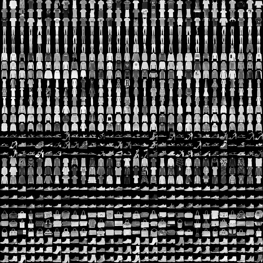
- [Fashion MNIST](https://github.com/zalandoresearch/fashion-mnist#fashion-mnist): 10-category classification.
{width=500px}
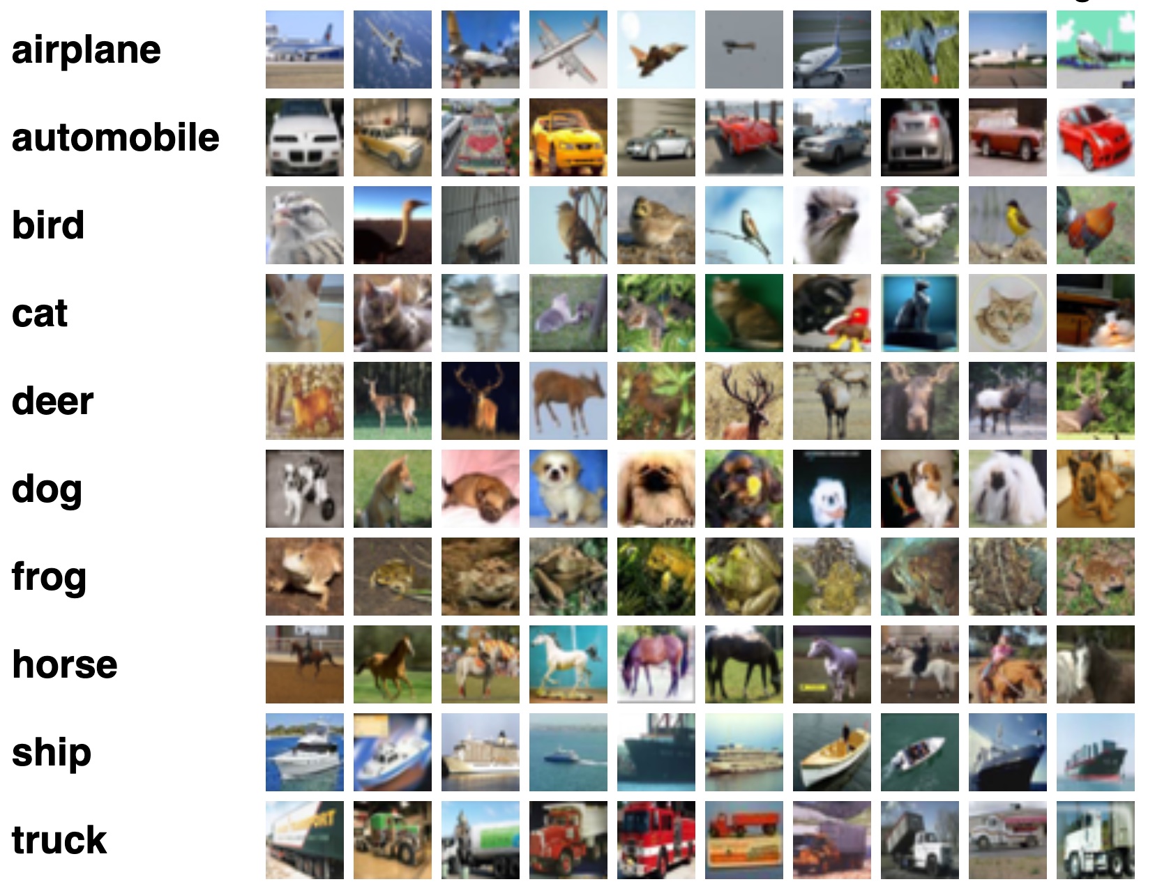
- [CIFAR-10 and CIFAR-100](https://www.cs.toronto.edu/~kriz/cifar.html)
{width=500px}
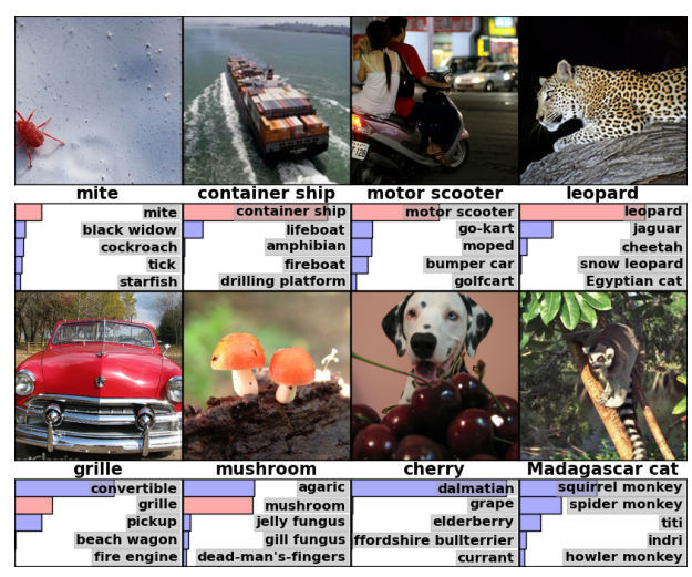
- [ImageNet](https://www.image-net.org/)
{width=500px}
- [Microsoft COCO](https://cocodataset.org/#home) (object detection, segmentation, and captioning)
{width=500px}
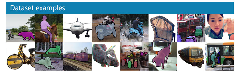
- [ADE20K](http://groups.csail.mit.edu/vision/datasets/ADE20K/) (scene parsing)
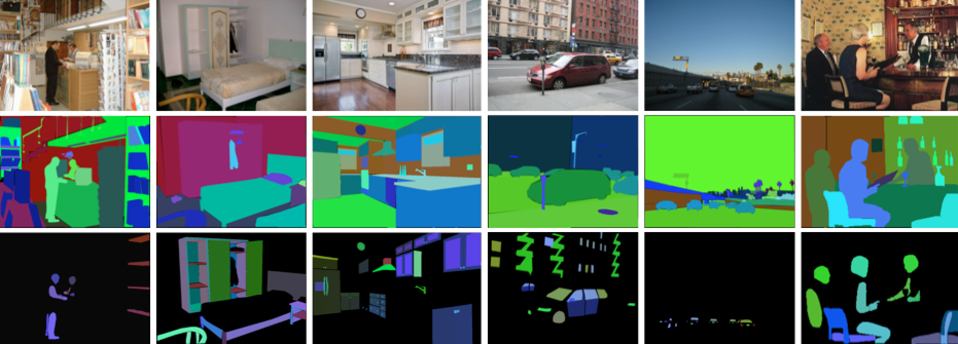{width=500px}
### Example: classify the pixels in a satellite image, by usage
::: {#fig-landsat}
{width=750px height=750px}
LANDSET images (ESL Figure 13.6).
:::
- LANDSAT: 82x100 pixels. Four heat-map images, two in the visible spectrum and two in the infrared, for an area of agricultural land in Australia.
- Each pixel has a class label from the 7-element set \{red soil, cotton, vegetation stubble, mixture, gray soil, damp gray soil, very damp gray soil\}, determined manually by
research assistants surveying the area. The objective is to classify the land usage at a pixel, based on the information in the four spectral bands.
## Unsupervised learning
- No outcome variable, just predictors.
- Objective is more fuzzy: find groups that behave similarly, find features that behave similarly, find linear combinations of features with the most variations, generative models (transformers).
- Difficult to know how well you are doing.
- Can be useful in exploratory data analysis (EDA) or as a pre-processing step for supervised learning.
### Example: gene expression
- The `NCI60` data set consists of 6,830 gene expression measurements for each of 64 cancer cell lines.
::: {.panel-tabset}
#### R
```{r}
# NCI60 data and cancel labels
str(NCI60)
# Cancer type of each cell line
table(NCI60$labs)
# Apply PCA using prcomp function
# Need to scale / Normalize as
# PCA depends on distance measure
prcomp(NCI60$data, scale = TRUE, center = TRUE, retx = T)$x %>%
as_tibble() %>%
add_column(cancer_type = NCI60$labs) %>%
# Plot PC2 vs PC1
ggplot() +
geom_point(mapping = aes(x = PC1, y = PC2, color = cancer_type)) +
labs(title = "Gene expression profiles cluster according to cancer types")
```
#### Python
```{python}
# Import NCI60 data
nci60_data = pd.read_csv('../data/NCI60_data.csv')
nci60_labs = pd.read_csv('../data/NCI60_labs.csv')
nci60_data.info()
```
```{python}
from sklearn.decomposition import PCA
from sklearn.preprocessing import scale
# Obtain the first 2 principal components
nci60_tr = scale(nci60_data, with_mean = True, with_std = True)
nci60_pc = pd.DataFrame(
PCA(n_components = 2).fit(nci60_tr).transform(nci60_tr),
columns = ['PC1', 'PC2']
)
nci60_pc['PC2'] *= -1 # for easier comparison with R
nci60_pc['cancer_type'] = nci60_labs
nci60_pc
```
```{python}
# Plot PC2 vs PC1
sns.relplot(
kind = 'scatter',
data = nci60_pc,
x = 'PC1',
y = 'PC2',
hue = 'cancer_type',
height = 10
)
```
:::
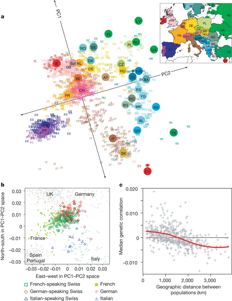
### Example: mapping people from their genomes
- The genetic makeup of $n$ individuals can be represented by a matrix @eq-predictor-matrix, where $x_{ij} \in \{0, 1, 2\}$ is the $j$-th genetic marker of the $i$-th individual.
Is that possible to visualize the geographic relationship of these individuals?
- Following picture is from the article [_Genes mirror geography within Europe_](http://www.nature.com/nature/journal/v456/n7218/full/nature07331.html) by Novembre et al (2008) published in Nature.
### Ancestry estimation
::: {#fig-open-admixture}
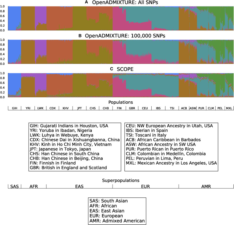{width=750px height=750px}
Unsupervised discovery of ancestry-informative markers and genetic admixture proportions. [Paper](https://doi.org/10.1016/j.ajhg.2022.12.008).
:::
## No easy answer
In modern applications, the line between supervised and unsupervised learning is blurred.
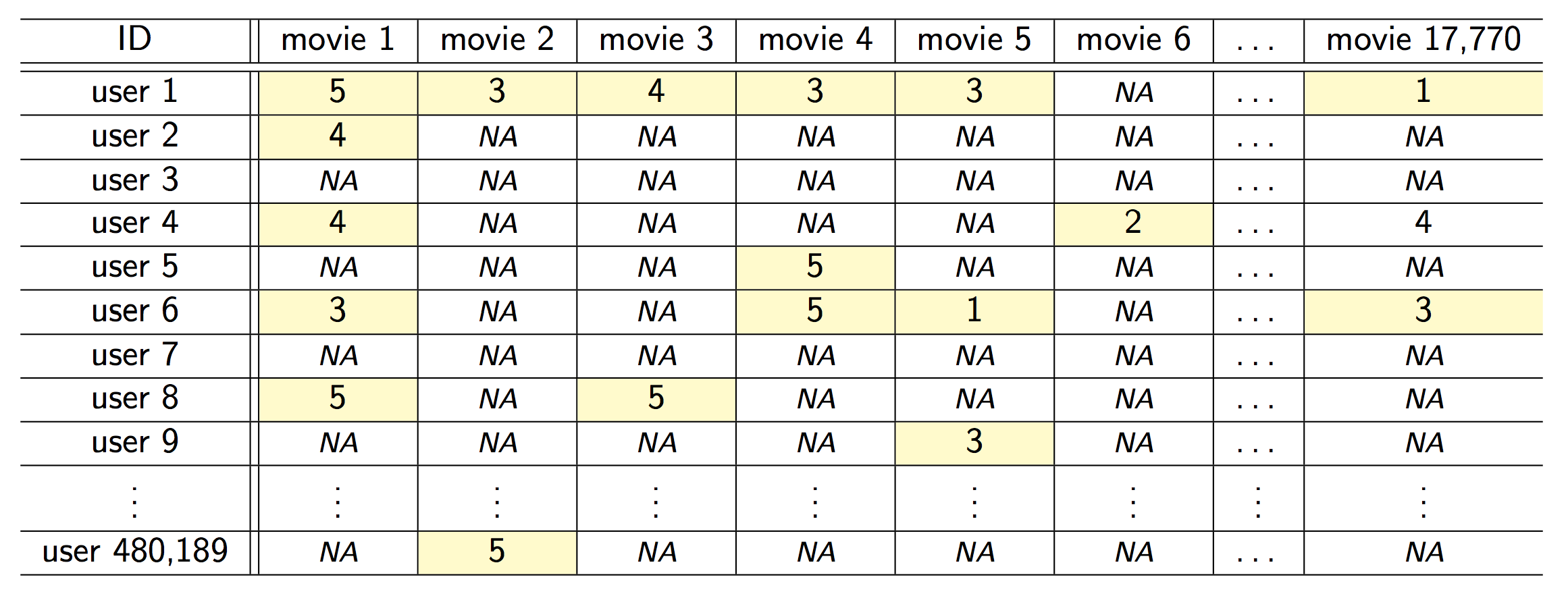
### Example: the Netflix prize
::: {#fig-netflix fig-ncols=1}
{fig-align="center"}
{fig-align="center"}
The Netflix challenge.
:::
- Competition started in Oct 2006. Training data is ratings for 480,189 Netflix customers $\times$ 17,770 movies, each rating between 1 and 5.
- Training data is very sparse, about 98\% sparse.
- The objective is to predict the rating for a set of 1 million customer-movie pairs that are missing in the training data.
- Netflix's in-house algorithm achieved a root MSE of 0.953. The first team to achieve a 10\% improvement wins one million dollars.
- Is this a supervised or unsupervised problem?
- We can treat `rating` as outcome and user-movie combinations as predictors. Then it is a supervised learning problem.
- Or we can treat it as a matrix factorization or low rank approximation problem. Then it is more of a unsupervised learning problem, similar to PCA.
### Example: large language models (LLMs)
Modern large language models, such as [ChatGPT o1](https://chat.openai.com), combine both supervised learning and reinforcement learning [google trends](https://trends.google.com/trends/explore?date=2022-11-01%202024-01-05&geo=US&q=chatgpt&hl=en)
## Statistical learning vs machine learning
- Machine learning arose as a subfield of Artificial Intelligence.
- Statistical learning arose as a subfield of Statistics.
- There is much overlap. Both fields focus on supervised and unsupervised problems.
- Machine learning has a greater emphasis on large scale applications and prediction accuracy.
- Statistical learning emphasizes models and their interpretability, and precision and uncertainty.
- But the distinction has become more and more blurred, and there is a great deal of "cross-fertilization".
- Machine learning has the upper hand in Marketing!
## A Brief History of Statistical Learning
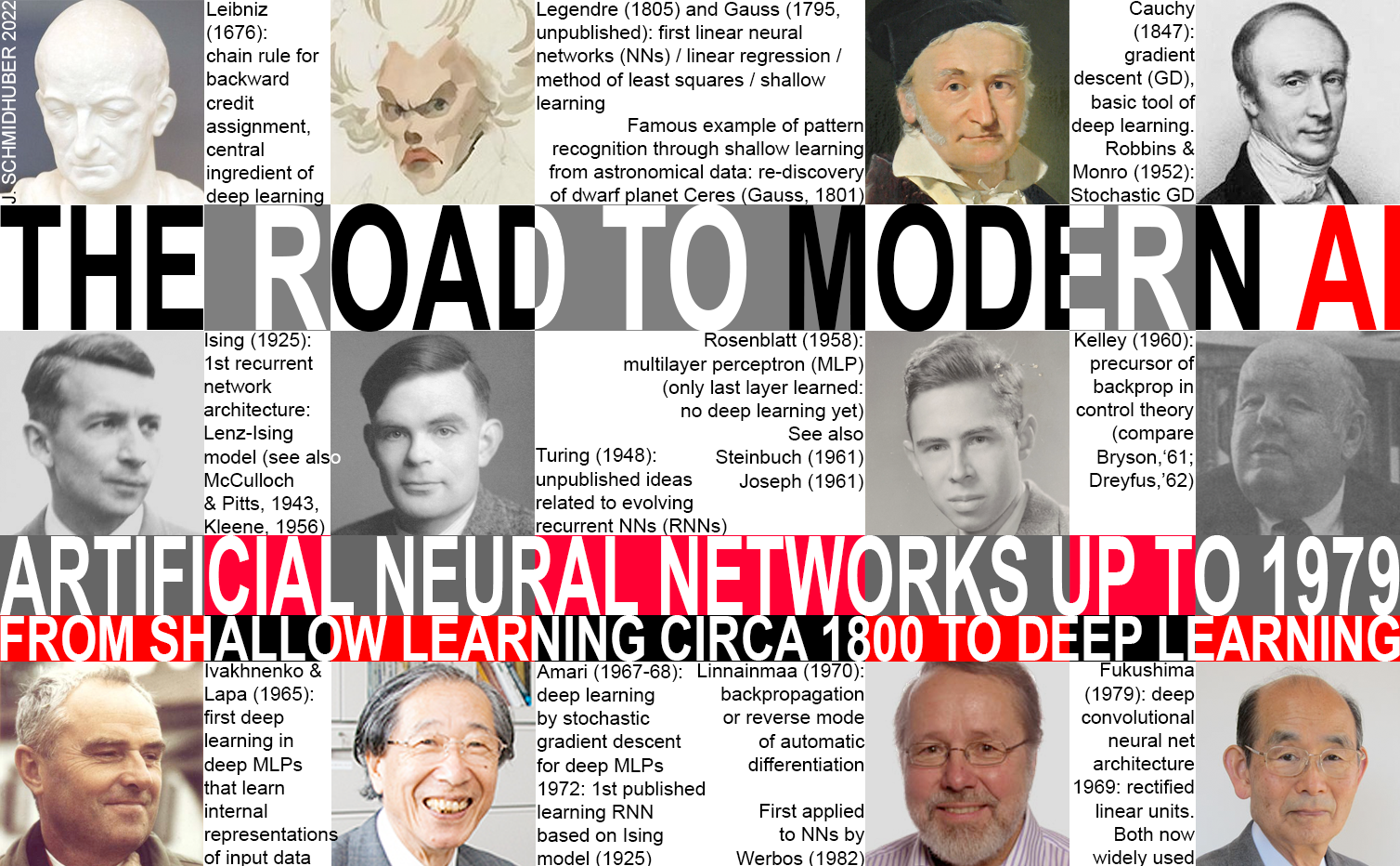
Image source:
- 1676, chain rule by Leibniz.
- 1805, least squares / linear regression / shallow learning by Gauss.
- 1936, classification by linear discriminant analysis by Fisher.
- 1940s, logistic regression.
- Early 1970s, generalized linear models (GLMs).
- Mid 1980s, classification and regression trees.
- 1980s, generalized additive models (GAMs).
- 1980s, neural networks gained popularity.
- 1990s, support vector machines.
- 2010s, deep learning.
# Course logistics
## Learning objectives
1. Understand what machine learning is (and isn't).
2. Learn some foundational methods/tools.
3. For specific data problems, be able to choose methods that make sense.
::: {.callout-tip}
Q: Wait, Dr. Zhou! Why don't we just learn the best method (aka deep learning) first?
A: No single method dominates. One method may prove useful in answering some questions on a given data set. On a related (not identical) data set or question, another might prevail. [Article](https://arxiv.org/abs/2106.03253)
:::
## Syllabus
- Read [syllabus](https://ucla-biostat-212a.github.io/2025winter/syllabus/syllabus.html) and [schedule](https://ucla-biostat-212a.github.io/2025winter/schedule/schedule.html) for a tentative list of topics and course logistics.
- Homework assignments will be a mix of theoretical/conceptual and applied/computational questions. Although not required, you are highly encouraged to practice literate programming (using Jupyter, Quarto, RMarkdown, or Google Colab) coordinated through Git/GitHub. This will enhance your GitHub profile and make you more appealing on job market.
- Although, I do not require homework submission through Git/Github. Homework submission is through BruinLearn.
- We will mainly use R in this course.
## What I expect from you
- You are curious and are excited about "figuring stuff out".
- You are proficient in coding and debugging (or are ready to work to get there).
- You have a solid foundation in introductory statistics (or are ready to work to get there).
- You are willing to ask questions.
## What you can expect from me
- I value your learning experience and process.
- I'm flexible with respect to the topics we cover.
- I'm happy to share my professional connections.
- I'll try my best to be responsive in class, in office hours, and other professional encounters.
# Notation and Simple Matrix Algebra
## Notation
- We will use $n$ to represent the number of distinct data points, or observations, in our sample.
- We will let $p$ denote the number of variables that are available for use in making predictions.
+ For example, the `Wage` data set consists of 11 variables for 3,000 people, so we have $n = 3,000$ observations and $p = 11$ variables (such as year, age, race, and more).
+ $p$ can be quite large, such as on the order of thousands or even millions, e.g., modern biological data, like gene expression, DNA sequences along the genome.
- We will let $x_{ij}$ represent the value of the $j$th variable for the $i$th observation, where $i = 1,2,\ldots,n$ and $j = 1,2,\ldots,p$.
- We will let $i$ be the index of the samples or observations (from 1 to $n$) and $j$ will be used to index the variables (from 1 to $p$).
- We let $\mathbf{X}$ denote an $n \times p$ matrix whose $(i, j )$th element is $x_{ij}$
$$
\mathbf{X} = \begin{pmatrix}
x_{11} & \cdots & x_{1p} \\
\vdots & \ddots & \vdots \\
x_{n1} & \cdots & x_{np}
\end{pmatrix} = \begin{pmatrix} \mathbf{x}_1^T \\ \vdots \\ \mathbf{x}_n^T \end{pmatrix}
$$
- Rows of X, which we write as $x_1, x_2, \ldots , x_n$. Here $x_i$ is a vector of length $p$, containing the $p$ variable measurements for the $i$th observation. That is,
$$
x_i = \begin{pmatrix} x_{i1} \\ \vdots \\ x_{ip} \end{pmatrix}.
$$
**Note: Vectors are by default represented as columns.**
- At other times we will instead be interested in the columns of $\mathbf{X}$, which we write as $\mathbf{x}_1,\mathbf{x}_2,\ldots,\mathbf{x}_p$. Each is a vector of length $n$. That is,
$$
\mathbf{x}_j = \begin{pmatrix} \mathbf{x}_{1j} \\ \vdots \\ \mathbf{x}_{nj} \end{pmatrix}.
$$
- Using this notation, the matrix $\mathbf{X}$ can be written as
$$
\mathbf{X} = (\mathbf{x}_1 \quad \mathbf{x}_2 \quad \ldots \quad \mathbf{x}_p),
$$
or
$$
\mathbf{X} = \begin{pmatrix} x_{1}^T \\ \vdots \\ x_{n}^T \end{pmatrix}.
$$
- We use $y_i$ to denote the $i$th observation of the variable on which we wish to make predictions (i.e., "outcome"), such as wage. Hence, we write the set of all $n$ observations in vector form as
$$
\mathbf{y} = \begin{pmatrix} y_1 \\ \vdots \\ y_n \end{pmatrix}
$$
Then our observed data consists of ${(x_1, y_1), (x_2, y_2), \ldots , (x_n, y_n)}$, where each $x_i$ is a vector of length $p$. (If $p = 1$, then $x_i$ is simply a scalar.)
## Matrix Algebra
- Matrices will be denoted using bold capitals, such as $\mathbf{A}$.
- To indicate that an object is a scalar, we will use the notation $a \in R$.
- To indicate that it is a vector of length $k$,we will use $\mathbf{a}\in R^k$ (or $\mathbf{a}\in R^n$ if it is of length $n$).
- We will indicate that an object is an $r \times s$ matrix using $\mathbf{A} \in R^{r\times s}$.
### Special cases of matrices
- A column vector is a matrix with only one column, e.g.
$$
\mathbf{A} = \left(\begin{array}{c}
1 \\
4 \\
0\\
-2\\
\end{array}\right)
$$
- A row vector is a matrix with only one row, e.g.
$$
\mathbf{A} = \left(\begin{array}{cccc}
1 & 4 & 0 & -2\\
\end{array}\right)
$$
- A matrix with $r = s$, that is, with the same number of rows and columns is called a **square matrix**. If a matrix \mathbf{A} is square, the elements $a_{ii}$ are said to lie on the **diagonal**
of \mathbf{A}.
$$
\mathbf{A} = \left(\begin{array}{cc}
1 & 4 \\
0 & -2
\end{array}\right)
$$
- A square matrix \mathbf{A} is called \alert{symmetric} if $a_{ij} = a_{ji}$ for all values of i and j.
$$
\mathbf{A} = \left(\begin{array}{ccc}
3 &5& 7 \\
5 &1& 4 \\
7 &4 &8
\end{array}\right)
$$
Symmetric matrices turn out to be quite important in formulating statistical models for all types of data!
- An important special case of a square, symmetric matrix is the identity matrix, i.e., a square matrix with $1$s on diagonal, $0$s elsewhere, e.g.
$$
\mathbf{A} = \left(\begin{array}{ccc}
1 & 0 & 0 \\
0 & 1 & 0 \\
0& 0& 1\\
\end{array}\right)
$$
The identity matrix functions the same way as "$1$" does in the real number system.
### Matrix operations
#### Transpose
- The $^T$ notation denotes the transpose of a matrix or vector
$$
\mathbf{X}^T = \begin{pmatrix}
x_{11} & \cdots & x_{1n} \\
\vdots & \ddots & \vdots \\
x_{p1} & \cdots & x_{pn}
\end{pmatrix} = \begin{pmatrix} \mathbf{x}_1^T \\ \vdots \\ \mathbf{x}_n^T \end{pmatrix}
$$
So the transpose of a $n\times p$ matrix is a $p\times n$ matrix. That is, the transpose of $A$ is the matrix found by ``flipping" the matrix around.
- For example,
$$
\mathbf{A} =
\left(
\begin{array}{ccc}
1 & 2 & 3 \\
4 & 5 & 6 \\
\end{array}
\right)
\quad
\mathbf{A}^T =
\left(
\begin{array}{cc}
1 & 4 \\
2 & 5 \\
3 & 6 \\
\end{array}
\right)
$$
A **fundamental property of a symmetric matrix** is that the matrix and its transpose are the same; i.e., if $\mathbf{A}$ is symmetric then $\mathbf{A} = \mathbf{A}^T$. (Try it on the symmetric matrix above.)
#### Matrix Addition and Subtraction
Adding or subtracting two matrices are operations that are defined **element-by-element**. That is, to add to matrices, add their corresponding elements, e.g.
$$
\mathbf{A} =
\left(
\begin{array}{cc}
1 & 2 \\
4 & 5 \\
\end{array}
\right)
\quad
\mathbf{B} =
\left(
\begin{array}{cc}
6 & 4 \\
2 & -1 \\
\end{array}
\right)
$$
Then,
$$
\mathbf{A} + \mathbf{B} =
\left(
\begin{array}{cc}
7 & 6 \\
6 & 4 \\
\end{array}
\right)
\quad
\mathbf{A} - \mathbf{B} =
\left(
\begin{array}{cc}
-5 &-2 \\
-2 & 6 \\
\end{array}
\right)
$$
- Note that these operations only make sense if the two matrices have the **same dimension**; the operations are not defined otherwise.
#### Matrix Multiplication
- The effect of multiplying a matrix $\mathbf{A}$ with any dimension by a real number (scalar) $b$, say, is to multiply each element in $\mathbf{A}$ by $b$.
$$
3\left(
\begin{array}{cc}
1 & 2 \\
4 & 5 \\
\end{array}
\right) =
\left(
\begin{array}{cc}
3 & 6 \\
12 & 15 \\
\end{array}
\right)
$$
- General rules,
+ $\mathbf{A} + \mathbf{B} = \mathbf{B} + \mathbf{A}$, $b(\mathbf{A} + \mathbf{B})=b\mathbf{A} + b\mathbf{B}$
+ $(\mathbf{A} + \mathbf{B})^T=\mathbf{A}^T + \mathbf{B}^T$, $(b\mathbf{A})^T=b\mathbf{A}^T$
- Order matters
+ Number of columns of first matrix must = Number of rows of second matrix, e.g.,
$$
\mathbf{A} = \left(
\begin{array}{ccc}
1 & 2 &5 \\
4 & 5 &1 \\
\end{array}
\right) \quad
\mathbf{B} = \left(
\begin{array}{cc}
3 & 6 \\
2 & 5 \\
1 & 2 \\
\end{array}
\right)\\ \quad
\mathbf{C} = (c_{ij}) = \mathbf{AB} = \left(
\begin{array}{cc}
12 & 26 \\
23 & 51 \\
\end{array}
\right)
$$
- Formally, if $\mathbf{A}$ is $(r\times s)$ and $\mathbf{B}$ is $(s\times q)$, then $\mathbf{AB}$ is a $(r\times q)$ matrix with $(i,j)$th element
$$
\sum_{k=1}^s a_{ik}b_{kj}.
$$
- General rules,
+ $\mathbf{A}(\mathbf{B} + \mathbf{C}) = \mathbf{A}\mathbf{B} + \mathbf{A}\mathbf{C}$, $(\mathbf{A}+\mathbf{B}) \mathbf{C} = \mathbf{A}\mathbf{C} + \mathbf{B}\mathbf{C}$
+ For any matrix $\mathbf{A}$, $\mathbf{A}^T\mathbf{A}$ will be a square matrix.
+ The transpose of a matrix product: $(\mathbf{AB})^T=\mathbf{B}^T\mathbf{A}^T$.
### Example
- Consider a prediction model, e.g., `wage` data example: suppose that we have $n$ pairs $(x_1,Y_1),\ldots,(x_n,Y_n)$, and we believe that, except for a random deviation, the relationship between the \alert{covariate} $x$ (e.g., `age`) and the response $\mathbf{Y}$ follows a straight line. That is, for $j=1,\ldots,n$, we have
$$
\mathbf{Y}_j = \beta_0 + \beta_1x_j + \epsilon_j,
$$
where $\epsilon_j$ is a random deviation representing the amount by which the actual observed response $Y_j$ deviates from the exact straight line relationship. Defining,
$$
\mathbf{X}= \left(
\begin{array}{cc}
1 & x_1 \\
1 & x_2 \\
\vdots & \vdots\\
1&x_n\\
\end{array}
\right),\quad
Y= \left(
\begin{array}{c}
Y_1 \\
Y_2 \\
\vdots \\
Y_n\\
\end{array}
\right),\quad
\epsilon= \left(
\begin{array}{c}
\epsilon_1 \\
\epsilon_2 \\
\vdots \\
\epsilon_n\\
\end{array}
\right),
\beta= \left(
\begin{array}{c}
\beta_0 \\
\beta_1 \\
\end{array}
\right),
$$
we may express the model succinctly as
$$
\mathbf{Y}=\mathbf{X}\beta +\epsilon.
$$