H$_0$: There is no relationship between $X$ and $Y$.
vs the **alternative** hypothesisH$_1$: There is some relationship between $X$ and $Y$.
+ Mathematically, this corresponds to testing $$ H_0: \beta_1 = 0 $$ vs the **alternative** hypothesis $$ H_1: \beta_1 \neq 0. $$ + In practice, we compute a t-statistic, given by $$ t = \frac{\beta_1-0}{\text{SE} (\beta_1)}, $$ which measures the number of standard deviations that $\beta_1$ is away from 0. + If there really is no relationship between $X$ and $Y$ (i.e., under the null hypothesis), then we expect that $t$ will follow a t-distribution with $n − 2$ degrees of freedom. - **P-value:** Assuming $\beta_1 = 0$, i.e., under the null hypothesis, the probability of observing any number equal to or larger than $|t|$. + Roughly, a small p-value indicates that it is unlikely to observe such a substantial association between the predictor and the response due to chance, in the absence of any real association between the predictor and the response. + Hence, if p-value is small, we can **infer** that there is an association between the predictor and the response. + That is we reject the null hypothesis and declare a relationship to exist between $X$ and $Y$. + How small is small? Typical p-value cutoffs for rejecting the null hypothesis are 5% or 1% (more discussions related to this topic will be discussed later). ### Assessing the accuracy of the model - Once we have rejected the null hypothesis in favor of the alternative hypothesis, how to quantify the extent to which the model fits the data? - The quality of a linear regression fit is typically assessed by: the residual standard error (RSE) and the R2 statistic. #### Residual standard error (RSE) - Recall that the RSE is an estimate of the standard deviation of $\epsilon$, and hence it is a measure of the **lack of fit** of the model to the data. $$ RSE = \sqrt{\frac{1}{n - 2} RSS} = \sqrt{\frac{1}{n - 2} \sum_{i=1}^{n} (y_i - \hat{y}_i)^2}. $$ ::: {.panel-tabset} #### R ```{r} library(gtsummary) fit <- lm(sales ~ TV, data = Advertising) fit %>% tbl_regression(estimate_fun = function(x) style_number(x, digits = 3), intercept = T) %>% bold_labels() %>% bold_p(t = 0.05) %>% modify_column_unhide(columns = c(statistic, std.error)) %>% add_glance_source_note( label = list(sigma ~ "\U03C3"), include = c(r.squared, sigma) ) ``` ::: > For the `advertising` data, actual sales in each market deviate from the true regression line by approximately 3,260 units, on average. To put in context of our outcome (i.e., sales): since the mean value of sales over all markets is approximately 14,000 units, the percentage error is 3,260/14,000 = 23 %. #### $R^2$ statistic - The $R^2$ statistic provides an alternative measure of fit. It takes the form of a **proportion** —the proportion of variance explained—and so it always takes on a value between 0 and 1, and is independent of the scale of Y. To calculate R2, we use the formula $$ R^2 = \frac{\text{TSS}-\text{RSS}}{\text{TSS}} = 1 - \frac{\text{RSS}}{\text{TSS}}, $$ where $\text{TSS} = \sum(y_i-\bar y)^2$ is the **total sum of squares**, and RSS is defined as above. + TSS measures the total variance in the response Y , and can be thought of as the amount of variability inherent in the response before the regression is performed. + RSS measures the amount of variability that is left unexplained after performing the regression. + Hence, TSS − RSS measures the amount of variability in the response that is explained (or removed) by performing the regression, and $R^2$ measures the proportion of variability in Y that can be explained using X. + An $R^2$ statistic that is close to 1 indicates that a large proportion of the variability in the response has been explained by the regression. + In contrast, a $R^2$ statistic that is close to 0 indicates that the regression did not explain much of the variability in the response, e.g., non-linear relationship between $X$ and $Y$ or error variance $\sigma^2$ is high. > In `advertising` data, the R2 was 0.61, and so just under two-thirds of the variability in sales is explained by a linear regression on TV. - What is a good $R^2$ value? + It depends on the application and the type of response that is being predicted, e.g., in typical applications in biology, psychology, marketing, and other domains, the linear model can only explain a small fraction of the total variability in the response. Therefore the $R^2$ can be below 0.1 which is realistic. - $R^2$ is closely related to the correlation between the response and the fitted linear model. + Recall that the correlation between two variables is given by $$ r = \text{Cor}(X, Y) = \frac{\sum_{i=1}^n (x_i - \bar x)(y_i - \bar y)}{\sqrt{\sum_{i=1}^n (x_i - \bar x)^2 \sum_{i=1}^n (y_i - \bar y)^2}}. $$ + In fact, it can be shown that in the simple linear regression setting, $R^2 = r^2$. ## Multiple linear regression - We estimate regression coefficients $\beta_0, \beta_1, \ldots, \beta_p$ by the **method of least squares**, which minimizes the sum of squared residuals \begin{align*} \text{RSS} & = \sum_{i=1}^n (y_i - \hat y_i)^2 = \sum_{i=1}^n (y_i - \beta_0 - \beta_1 x_{i1} - \cdots - \beta_p x_{ip})^2.\\ & = (\mathbf{y} - \mathbf{X} \beta)^T (\mathbf{y} - \mathbf{X} \beta). \end{align*} - The minimizer $\hat \beta_0, \hat \beta_1, \ldots, \hat \beta_p$ admits the analytical solution $$ \hat \beta = (\mathbf{X}^T \mathbf{X})^{-1} \mathbf{X}^T \mathbf{y}. $$ and we can make prediction using the formula $$ \hat y = \hat \beta_0 + \hat \beta_1 x_1 + \cdots + \hat \beta_p x_p. $$ ::: {.panel-tabset} #### R ```{r} library(gtsummary) # Linear regression lmod <- lm(sales ~ TV + radio + newspaper, data = Advertising) summary(lmod) ``` ```{r} # Better summary table lmod %>% tbl_regression() %>% bold_labels() %>% bold_p(t = 0.05) %>% modify_column_unhide(columns = c(statistic, std.error)) %>% add_glance_source_note( label = list(sigma ~ "\U03C3"), include = c(r.squared, sigma) ) ``` #### Python (sklearn) ```{python} # sklearn does not offer much besides coefficient estimate from sklearn.linear_model import LinearRegression X = Advertising[['TV', 'radio', 'newspaper']] y = Advertising['sales'] lmod = LinearRegression().fit(X, y) lmod.intercept_ lmod.coef_ # Score is the R^2 lmod.score(X, y) ``` #### Python (statsmodels) ```{python} import statsmodels.api as sm import statsmodels.formula.api as smf # Fit linear regression lmod = smf.ols(formula = 'sales ~ TV + radio + newspaper', data = Advertising).fit() lmod.summary() ``` ::: ## Interpreting regression coefficients - We interpret $\beta_j$ as the average effect on $Y$ of a one-unit increase in $X_j$, _holding all other predictors fixed_. > a regression coefficient $\beta_j$ estimates the expected change in $Y$ per unit change in $X_j$, with all other predictors held fixed. But predictors usually change together! > > "Data Analysis and Regression", Mosteller and Tukey 1977 - Only when the predictors are uncorrelated, each coefficient can be estimated, interpreted, and tested separately. In other words, only when the predictors are uncorrelated, the regression coefficients estimated from multiple linear regression are the same as those from separate simple linear regressions. - Claims of **causality** should be avoided for observational data. ::: {.panel-tabset} #### R ```{r} # install.packages("corrr") library(corrr) # Correlation matrix Advertising %>% select(sales, TV, radio, newspaper) %>% correlate() ``` ::: > So newspaper advertising is a surrogate for radio advertising; newspaper gets “credit” for the association between radio on sales. This is called **confounding**. ## Some important questions ### Goodness of fit **Question:** Is at least one of the predictors $X_1, X_2, \ldots, X_p$ useful in predicting the response? - We can use the F-statistic to assess the fit of the overall model. Formally we are testing the null hypothesis $$ H_0: \beta_1 = \cdots = \beta_p = 0 $$ versus the alternative $$ H_a: \text{at least one } \beta_j \text{ is non-zero}. $$ F-statistic is defined as $$ F = \frac{(\text{TSS} - \text{RSS})/p}{\text{RSS}/(n-p-1)} \sim F_{p, n-p-1}, $$ where $$ \text{TSS} = \sum_{i=1}^n (y_i - \bar y)^2. $$ If the linear model assumptions are correct, one can show that $$ \mathbf{E}{\text{RSS}/(n − p − 1)} = \sigma^2 $$ and that, provided $H_0$ is true, $$ \mathbf{E}{(\text{TSS} − \text{RSS})/p} = \sigma^2. $$ Hence, when there is no relationship between the response and predictors, F-statistic to take on a value close to 1. On the other hand, if $H_a$ is true, then $\mathbf{E}{(\text{TSS} − \text{RSS})/p} > \sigma^2$, so we expect F to be greater than 1. - The p-value for the F-statistic is computed using the F-distribution with $p$ and $n-p-1$ degrees of freedom. - In general, the F-statistic for testing $$ H_0: \text{ a restricted model } \omega $$ versus $$ H_a: \text{a more general model } \Omega $$ takes the form $$ F = \frac{(\text{RSS}_\omega - \text{RSS}_\Omega) / (\text{df}(\Omega) - \text{df}(\omega))}{\text{RSS}_\Omega / (n - \text{df}(\Omega))}, $$ where df is the degree of freedom (roughly speaking the number of free parameters) of a model. ::: {.panel-tabset} #### R ```{r} lmod_null <- lm(sales ~ 1, data = Advertising) anova(lmod_null, lmod) ``` #### Python (statsmodels) ```{python} # F test for R \beta = 0 R = [[0, 1, 0 , 0], [0, 0, 1, 0], [0, 0, 0, 1]] lmod.f_test(R) ``` the p-value associated with the F -statistic is essentially zero, so we have extremely strong evidence that at least one of the media is associated with increased sales. ::: ### Model selection **Question:** Do all the predictors help to explain $Y$ , or is only a subset of the predictors useful? - For a naive implementation of the best subset, forward selection, and backward selection regressions in Python, interesting readers can read this [blog](https://xavierbourretsicotte.github.io/subset_selection.html). #### Best subset regression - The most direct approach is called **all subsets** or **best subsets** regression: we compute the least squares fit for all possible subsets and then choose between them based on some criterion that balances training error with model size. - We try the highly-optimized [`abess`](https://abess.readthedocs.io/en/latest/index.html) package here. ::: {.panel-tabset} #### R ```{r} library(leaps) bs_mod <- regsubsets( sales ~ ., data = Advertising, method = "exhaustive" ) %>% summary() bs_mod tibble( K = 1:3, R2 = bs_mod$rsq, adjR2 = bs_mod$adjr2, BIC = bs_mod$bic, CP = bs_mod$cp ) %>% print(width = Inf) ``` #### Python ```{python, eval = FALSE} from abess.linear import LinearRegression from patsy import dmatrices # Create design matrix and response vector using R-like formula ym, Xm = dmatrices( 'sales ~ TV + radio + newspaper', data = Advertising, return_type = 'matrix' ) lmod_abess = LinearRegression(support_size = range(3)) lmod_abess.fit(Xm, ym) lmod_abess.coef_ ``` ::: - However we often can't examine all possible models, since there are $2^p$ of them. For example, when $p = 30$, there are $2^{30} = 1,073,741,824$ models! - Recent advances make possible to solve best subset regression with $p \sim 10^3 \sim 10^5$ with high-probability guarantee of optimality. See this [article](https://doi.org/10.1073/pnas.2014241117). - For really big $p$, we need some heuristic approaches to search through a subset of them. We discuss three commonly use approaches next. #### Forward selection - Begin with the **null model**, a model that contains an intercept but no predictors. - Fit $p$ simple linear regressions and add to the null model the variable that results in the lowest RSS (equivalently the lowest AIC). - Add to that model the variable that results in the lowest RSS among all two-variable models. - Continue until some stopping rule is satisfied, for example when the AIC does not decrease anymore. ::: {.panel-tabset} #### R ```{r} step(lmod_null, scope = list(lower = sales ~ 1, upper = sales ~ TV + radio + newspaper), trace = TRUE, direction = "forward" ) ``` ::: #### Backward selection - Start with all variables in the model. - Remove the variable with the largest $p$-value. That is the variable that is the least statistically significant. - The new $(p-1)$-variable model is fit, and the variable with the largest p-value is removed. - Continue until a stopping rule is reached. For instance, we may stop when AIC does not decrease anymore, or when all remaining variables have a significant $p$-value defined by some significance threshold. - Backward selection cannot start with a model with $p > n$. ::: {.panel-tabset} #### R ```{r} step(lmod, scope = list(lower = sales ~ 1, upper = sales ~ TV + radio + newspaper), trace = TRUE, direction = "backward" ) ``` ::: #### Mixed selection - We alternately perform forward and backward steps until all variables in the model have a sufficiently low $p$-value, and all variables outside the model would have a large $p$-value if added to the model. ::: {.panel-tabset} #### R ```{r} step(lmod_null, scope = list(lower = sale ~ 1, upper = sale ~ TV + radio + newspaper), trace = TRUE, direction = "both" ) ``` ::: #### Other model selection criteria Commonly used model selection criteria include Mallow's $C_p$, Akaike information criterion (AIC), Bayesian information criterion (BIC), adjusted $R^2$, and cross-validation (CV). ### Model fit **Question:** How well does the selected model fit the data? - **$R^2$**: the fraction of variance explained $$ R^2 = 1 - \frac{\text{RSS}}{\text{TSS}} = 1 - \frac{\sum_i (y_i - \hat y_i)^2}{\sum_i (y_i - \bar y)^2}. $$ It turns out (HW1 bonus question) $$ R^2 = \operatorname{Cor}(Y, \hat Y)^2. $$ Adding more predictors into a model **always** increase $R^2$. - From computer output, we see the fitted linear model by using `TV`, `radio`, and `newspaper` has an $R^2=0.8972$. ::: {.panel-tabset} #### R ```{r} # R^2 summary(lmod)$r.squared # Cor(Y, \hat Y)^2 cor(predict(lmod), Advertising$sales)^2 ``` #### Python ```{python} # R^2 lmod.rsquared # Cor(Y, \hat Y)^2 np.corrcoef(Advertising['sales'], lmod.predict()) np.corrcoef(Advertising['sales'], lmod.predict())[0, 1]**2 ``` ::: - The **adjusted $R_a^2$** adjusts to the fact that a larger model also uses more parameters. $$ R_a^2 = 1 - \frac{\text{RSS}/(n-p-1)}{\text{TSS}/(n-1)}. $$ Adding a predictor will only increase $R_a^2$ if it has some predictive value. ::: {.panel-tabset} #### R ```{r} # Adjusted R^2 summary(lmod)$adj.r.squared ``` #### Python ```{python} # Adjusted R^2 lmod.rsquared_adj ``` ::: - The **rooted squared error (RSE)** $$ \text{RSE} = \sqrt{\frac{\text{RSS}}{n - p - 1}} $$ is an estimator of the noise standard error $\sqrt{\operatorname{Var}(\epsilon)}$. The smaller RSE, the better fit of the model. ### Prediction **Question:** Given a set of predictor values, what response value should we predict, and how accurate is our prediction? - Given a new set of predictors $x$, we predict $y$ by $$ \hat y = \hat \beta_0 + \hat \beta_1 x_1 + \cdots + \hat \beta_p x_p. $$ - Under the selected model $$ \text{sales} \approx \beta_0 + \beta_1 \times \text{TV} + \beta_2 \times \text{radio}, $$ how many units of sale do we expect with \$100k budget in `TV` and \$20k budget in `radio`? ::: {.panel-tabset} #### R ```{r} x_new <- list(TV = 100, radio = 20) lmod_small <- lm(sales ~ TV + radio, data = Advertising) predict(lmod_small, x_new, interval = "confidence") predict(lmod_small, x_new, interval = "prediction") ``` #### Python ```{python} from patsy import dmatrices # Create design matrix and response vector using R-like formula y_small, X_small = dmatrices( 'sales ~ TV + radio', data = Advertising, return_type = 'dataframe' ) # Fit linear regression lmod_small = sm.OLS(y_small, X_small).fit() lmod_small_pred = lmod_small.get_prediction(pd.DataFrame({'Intercept': [1], 'TV': [100], 'radio': [20]})).summary_frame() lmod_small_pred ``` ::: - 95\% **Confidence interval**: probability of covering the true $f(X)$ is 0.95. - 95\% **Predictive interval**: probability of covering the true $Y$ is 0.95. Predictive interval is always wider than the confidence interval because it incorporates the randomness in both $\hat \beta$ and $\epsilon$. ## Qualitative (or categorical) predictors - In the `Advertising` data, all predictors are quantitative (or continuous). - The `Credit` data has a mix of quantitative (`Balance`, `Age`, `Cards`, `Education`, `Income`, `Limit`, `Rating`) and qualitative predictors (`Own`, `Student`, `Married`, `Region`). + `balance`: average credit card debt for each individual + quantitative predictors: `age`, `cards` (number of credit cards), `education` (years of education), `income` (in thousands of dollars), `limit` (credit limit), and `rating` (credit rating) + qualitative variables: `own` (house ownership), `student` (student status), `status` (marital status), and `region` (East, West or South). ::: {.panel-tabset} #### R ```{r} library(ISLR2) # Credit Credit <- as_tibble(Credit) %>% print(width = Inf) # Pair plot of continuous predictors ggpairs( data = Credit[, c(1:6, 11)], mapping = aes(alpha = 0.25) ) + labs(title = "Credit Data") # Pair plot of categorical predictors ggpairs( data = Credit[, c(7:10, 11)], mapping = aes(alpha = 0.25) ) + labs(title = "Credit Data") ``` #### Python ```{python} # Import Credit data Credit = pd.read_csv("../data/Credit.csv") Credit ``` ```{python} # Visualization by pair plot sns.pairplot(data = Credit) ``` ::: - By default, most software create **dummy variables**, also called **one-hot coding**, for categorical variables. Both Python (statsmodels) and R use the first level (in alphabetical order) as the base level. + For example: `own` has two levels: `no` and `yes`. The dummy variable `own` is 1 if `own` is `yes` and 0 otherwise: $$ x_i = \begin{cases} 1 & \text{if own}_i = \text{yes, } \text{i.e., if ith person owns a house} \\ 0 & \text{if own}_i = \text{no, } \text{i.e., if ith person does not own a house} \end{cases} $$ This results in the model $$ y_i = \beta_0 + \beta_1x_i + \epsilon = \begin{cases} \beta_0 + \beta_1 + \epsilon & \text{if own}_i = \text{yes, } \text{i.e., if ith person owns a house} \\ \beta_0 + \epsilon & \text{if own}_i = \text{no, } \text{i.e., if ith person does not own a house} \end{cases} $$ + $\beta_0$: the average credit card balance among those who do not own + $\beta_0 + \beta_1$: the average credit card balance among those who do own their house + $\beta_1$: the average difference in credit card balance between owners and non-owners + Since the p-value for the dummy variable is very high, this indicates that there is no statistical evidence of a difference in average credit card balance based on house ownership. ::: {.panel-tabset} #### R ```{r} lm(Balance ~ ., data = Credit) %>% tbl_regression() %>% bold_labels() %>% bold_p(t = 0.05) ``` #### Python ```{python} # Hack to get all predictors my_formula = "Balance ~ " + "+".join(Credit.columns.difference(["Balance"])) # Create design matrix and response vector using R-like formula y, X = dmatrices( my_formula, data = Credit, return_type = 'dataframe' ) # One-hot coding for categorical variables X ``` ```{python} # Fit linear regression sm.OLS(y, X).fit().summary() ``` ::: - There are many different ways of coding qualitative variables, measuring particular **contrasts**. + For example, instead of 0/1 coding scheme, we could create a dummy variable as: `own` is 1 if `own` is `yes` and -1 otherwise: $$ x_i = \begin{cases} 1 & \text{if own}_i = \text{yes, } \text{i.e., if ith person owns a house} \\ -1 & \text{if own}_i = \text{no, } \text{i.e., if ith person does not own a house} \end{cases} $$ This results in the model $$ y_i = \beta_0 + \beta_1x_i + \epsilon = \begin{cases} \beta_0 + \beta_1 + \epsilon & \text{if own}_i = \text{yes, } \text{i.e., if ith person owns a house} \\ \beta_0 -\beta_1 \epsilon & \text{if own}_i = \text{no, } \text{i.e., if ith person does not own a house} \end{cases} $$ + Question: how to interpret $\beta_0$ and $\beta_1$? ### More than two levels - When a qualitative predictor has more than two levels, more dummy variables is needed to represent all possible values. - For example, for the `region` variable we create two dummy variables: $$ x_{i1} = \begin{cases} 1 & \text{ if ith person is from South} \\ 0 & \text{ if ith person is not from South} \end{cases} $$ and $$ x_{i2} = \begin{cases} 1 & \text{ if ith person is from West} \\ 0 & \text{ if ith person is not from West} \end{cases} $$ This results in $$ y_i = \beta_0 + \beta_1x_{i1} + \beta_2x_{i2} + \epsilon = \begin{cases} \beta_0 + \beta_1 + \epsilon & \text{ if ith person is from South} \\ \beta_0 + \beta_2 + \epsilon & \text{ if ith person is from West}\\ \beta_0 + \epsilon & \text{ if ith person is from East} \end{cases} $$ - Question: how to interpret $\beta_0$, $\beta_1$, and $\beta_2$? - There will always be **one fewer** dummy variable than the number of levels. - The level with no dummy variable (i.e., East) is known as the **baseline** or **reference** level. - The choice of reference level depends on the question. It doesn't impact the prediction. But it will impact the value of coefficients and their p-values. - Use $F$-test to test $\beta_1=\beta_2=0$ ## Interactions - In our previous analysis of the `Advertising` data, we assumed that the effect on `sales` of increasing one advertising medium is independent of the amount spent on the other media $$ \text{sales} \approx \beta_0 + \beta_1 \times \text{TV} + \beta_2 \times \text{radio}. $$ - But suppose that spending money on radio advertising actually increases the effectiveness of TV advertising, so that the slope term for `TV` should increase as `radio` increases. - In this situation, given a fixed budget of $100,000, spending half on `radio` and half on `TV` may increase sales more than allocating the entire amount to either `TV` or to `radio`. - In marketing, this is known as a **synergy** effect, and in statistics it is referred to as an **interaction** effect. - Assume the interaction model: $$ \text{sales} \approx \beta_0 + \beta_1 \times \text{TV} + \beta_2 \times \text{radio} + \beta_3 \times (\text{TV} \times \text{radio}). $$ ::: {.panel-tabset} #### R ```{r} lmod_int <- lm(sales ~ 1 + TV * radio, data = Advertising) summary(lmod_int) lmod_int %>% tbl_regression(estimate_fun = function(x) style_sigfig(x, digits = 4)) %>% bold_labels() %>% bold_p(t = 0.05) ``` #### Python ```{python} # Design matrix with interaction y, X_int = dmatrices( 'sales ~ 1 + TV * radio', data = Advertising, return_type = 'dataframe' ) # Fit linear regression with interaction sm.OLS(y, X_int).fit().summary() ``` ::: - The results in this table suggests that the TV $\times$ Radio interaction is important. - The $R^2$ for the interaction model is 96.8\%, compared to only 89.7\% for the model that predicts sales using `TV` and `radio` without an interaction term. - This means that (96.8 - 89.7)/(100 - 89.7) = 69\% of the variability in sales that remains after fitting the additive model has been explained by the interaction term. - The coefficient estimates in the table suggest that an increase in TV advertising of \$1,000 is associated with increased sales of $$ (\hat \beta_1 + \hat \beta_3 \times \text{radio}) \times 1000 = 19 + 1.1 \times \text{radio units}. $$ - An increase in radio advertising of \$1,000 will be associated with an increase in sales of $$ (\hat \beta_2 + \hat \beta_3 \times \text{TV}) \times 1000 = 29 + 1.1 \times \text{TV units}. $$ - Sometimes it is the case that an interaction term has a very small p-value, but the associated main effects (in this case, `TV` and `radio`) do not. The **hierarchy principle** staties > If we include an interaction in a model, we should also include the main effects, even if the $p$-values associated with their coefficients are not significant. - The rationale for this principle is that interactions are hard to interpret in a model without main effects -- their meaning is changed. Specifically, the interaction terms still contain main effects, if the model has no main effect terms. ### Interaction between a qualitative variable and a quantitative variable - Consider the `Credit` data set, let's predict balance using the income (quantitative) and student (qualitative) variables. + In the absence of an interaction term, the model takes the form \begin{align*} \text{balance}_i &\approx \beta_0 + \beta_1 \times \text{income}_i + \begin{cases} \beta_2 & \text{ if ith person is a student}\\ 0 & \text{ if ith person is not a student} \end{cases}\\ &= \beta_1 \times \text{income}_i + \begin{cases} \beta_0+\beta_2 & \text{ if ith person is a student}\\ \beta_0 & \text{ if ith person is not a student} \end{cases} \end{align*} + With an interaction term, i.e., a change in income may have a very different effect on the credit card balance of a student versus a non-student. \begin{align*} \text{balance}_i &\approx \beta_0 + \beta_1 \times \text{income}_i + \begin{cases} \beta_2 + \beta_3 \times \text{income}_i& \text{ if ith person is a student}\\ 0 & \text{ if ith person is not a student} \end{cases}\\ &= \begin{cases} \beta_0+\beta_2 + (\beta_1 + \beta_3) \times \text{income}_i& \text{ if ith person is a student}\\ \beta_0 + \beta_1 \times \text{income}_i& \text{ if ith person is not a student} \end{cases} \end{align*}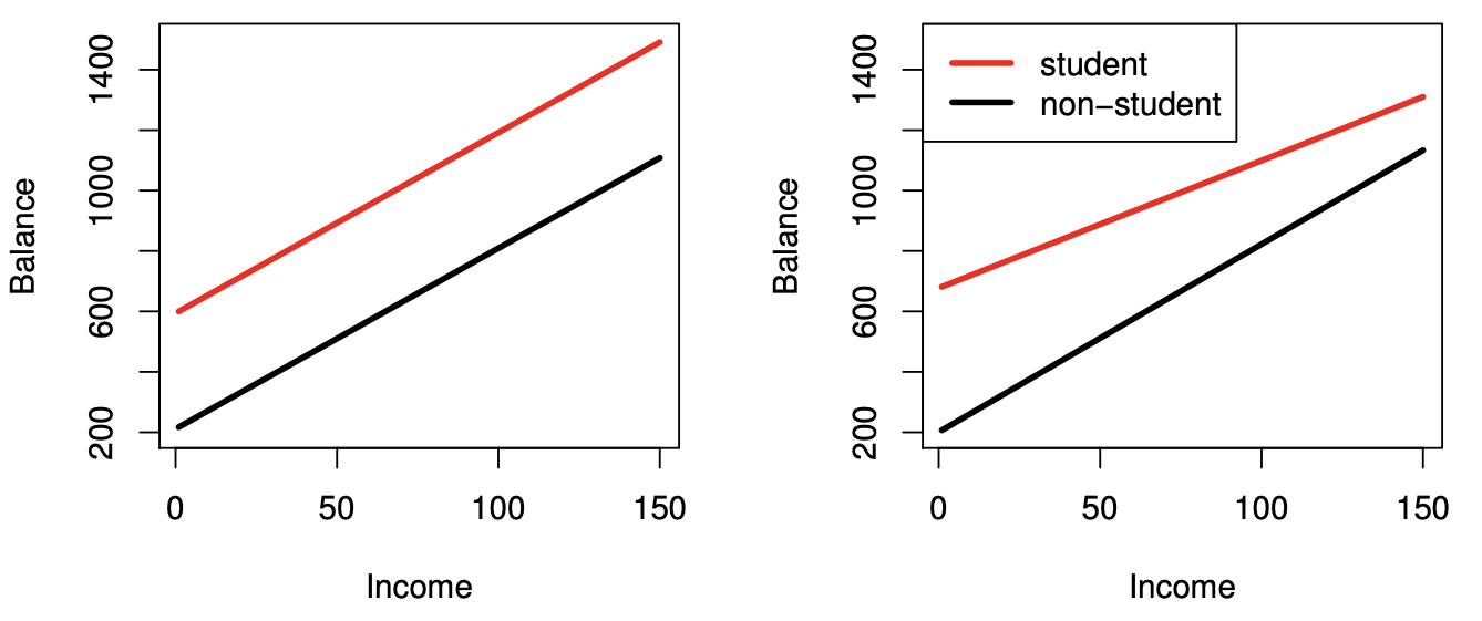{width=800px height=350px}
## Potential Problems ### Non-linear effects of predictors - Assumption for the linear regression model: there is a straight-line relationship between the predictors and the response. What if the data violates this assumptions? - `Auto` data. - Linear fit vs polynomial fit. ::: {.panel-tabset} #### R ```{r} ggplot(data = Auto, mapping = aes(x = horsepower, y = mpg)) + geom_point() + geom_smooth(method = lm, color = 1) + geom_smooth(method = lm, formula = y ~ poly(x, 2), color = 2) + geom_smooth(method = lm, formula = y ~ poly(x, 5), color = 3) + labs(x = "Horsepower", y = "Miles per gallon") ``` ::: The figure suggests that `mpg` vs `horsepower` to have a quadratic shape. And the following model $$ \text{mpg} = \beta_0 + \beta_1 \times \text{horsepower} + \beta_2 \times \text{horsepower}^2 + \epsilon $$ may provide a better fit. But it is still a linear model! So we can use standard linear regression software to estimate $\beta_0$, $\beta_1$, $\beta_2$ in order to produce a non-linear fit. ::: {.panel-tabset} #### R ```{r} Auto <- as_tibble(Auto) %>% print(width = Inf) # Linear fit lm(mpg ~ horsepower, data = Auto) %>% summary() # Degree 2 lm(mpg ~ poly(horsepower, 2), data = Auto) %>% summary() # Degree 5 lm(mpg ~ poly(horsepower, 5), data = Auto) %>% summary() ``` #### Python ```{python} # Import Auto data (missing data represented by '?') Auto = pd.read_csv("../data/Auto.csv", na_values = '?').dropna() Auto ``` ```{python} plt.clf() # Linear fit ax = sns.regplot( data = Auto, x = 'horsepower', y = 'mpg', order = 1 ) # Quadratic fit sns.regplot( data = Auto, x = 'horsepower', y = 'mpg', order = 2, ax = ax ) # 5-degree fit sns.regplot( data = Auto, x = 'horsepower', y = 'mpg', order = 5, ax = ax ) ax.set( xlabel = 'Horsepower', ylabel = 'Miles per gallon' ) ``` ::: #### Residual Plots - A useful graphical tool for identifying non-linearity, outliers, etc. - Recall residuals are $$ \epsilon_i = y_i - \hat{y}_i $$ Predicted/fitted values are $$ \hat{y}_i = \mathbf{X}\hat{\beta} $$ - We plot the residuals versus the predicted (or fitted) values ```{r} # Linear fit lm.fit <- lm(mpg ~ horsepower, data = Auto) plot(lm.fit, which = c(1)) ``` Ideally, the residual plot will show no discernible pattern. The presence of a pattern may indicate a problem with some aspect of the linear model. ```{r} # Linear fit lm.df2.fit <- lm(mpg ~ poly(horsepower, 2), data = Auto) plot(lm.df2.fit, which = c(1)) ``` If the residual plot indicates that there are non-linear associations in the data, then a simple approach is to use non-linear transformations of the predictors, such as $\text{log}X$, $\sqrt{X}$, and $X^2$, in the regression model. ### Correlation of error terms. - One important assumption of the linear regression model is that the error terms, $\epsilon_1, \ldots, \epsilon_n$, are uncorrelated, e.g., longitudinal data, time series data, etc. ### Non-constant variance of error terms. - Another important assumption of the linear regression model is that the error terms have a constant variance, $\text{Var}(\epsilon_i) = \sigma^2$. - Residual plot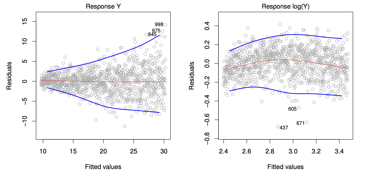{width=560px height=300px}
- Transformation of outcome or weighted least squares. ### Outliers. ### High leverage points. ### Collinearity. - Collinearity refers to the situation in which two or more predictor variables are closely related to one another. ```{r} library(ggplot2) ggplot(Credit, aes(x = Limit, y = Age)) + # Set up canvas with outcome variable on y-axis geom_point( color = "red") + scale_x_continuous(breaks = seq(2000, 12000, by = 2000)) + # Set x-axis limits scale_y_continuous(breaks = seq(30, 80, by = 10)) + xlab("Limit") + ylab("Age") + theme_bw() + theme(panel.background = element_rect(colour = "black", linewidth = 1), panel.grid.major = element_blank(), panel.grid.minor = element_blank(), axis.line = element_line(colour = "black")) ggplot(Credit, aes(x = Limit, y = Rating)) + # Set up canvas with outcome variable on y-axis geom_point( color = "red") + scale_x_continuous(breaks = seq(2000, 12000, by = 2000)) + # Set x-axis limits scale_y_continuous(breaks = seq(200, 800, by = 200)) + xlab("Limit") + ylab("Rating") + theme_bw() + theme(panel.background = element_rect(colour = "black", linewidth = 1), panel.grid.major = element_blank(), panel.grid.minor = element_blank(), axis.line = element_line(colour = "black")) ``` - Collinearity reduces the accuracy of the estimates of the regression coefficients, it causes the standard error to grow. - The power of the hypothesis test—the probability of correctly detecting a non-zero coefficient—is reduced by collinearity. - Solution: + drop one of the problematic variables from the regression. + combine the collinear variables together into a single predictor. ## Generalizations of linear models In much of the rest of this course, we discuss methods that expand the scope of linear models and how they are fit. - Classification problems: logistic regression, discriminant analysis, support vector machines. - Non-linearity: kernel smoothing, splines and generalized additive models, nearest neighbor methods. - Interactions: tree-based methods, bagging, random forests, boosting, neural networks. - Regularized fitting: ridge regression and lasso.